Bridging satellite missions: deep transfer learning for enhanced tropical cyclone intensity estimation

ABSTRACT

Geostationary satellites are valuable tools for monitoring the entire lifetime of tropical cyclones (TCs). Although the most widely used method for TC intensity estimation is manual, several automatic methods, particularly artificial intelligence (AI)-based algorithms, have been proposed and have achieved significant performance. However, AI-based techniques often require large amounts of input data, making it challenging to adopt newly introduced data such as those from recently launched satellites. This study proposed a transfer-learning-based TC intensity estimation method to combine different source data. The pre-trained model was built using the Swin Transformer (Swin-T) model, utilizing data from the Communication Ocean and Meteorological Satellite Meteorological Imager sensor, which has been in operation for an extensive period (2011–2021) and provides a large dataset. Subsequently, a transfer learning model was developed by fine-tuning the pre-trained model using the GEO-KOMPSAT-2A Advanced Meteorological Imager, which has been operational since 2019. The transfer learning approach was tested in three different ways depending on the fine-tuning ratio, with the optimal performance achieved when all layers were fine-tuned. The pre-trained model employed TC observations from 2011 to 2017 for training and 2018 for testing, whereas the transfer learning model utilized data from 2019 and 2020 for training and 2021 for testing to evaluate the model performance. The best pre-trained and transfer learning models achieved mean absolute error of 6.46 kts and 6.48 kts, respectively. Our proposed model showed a 7–52% improvement compared to the control models without transfer learning. This implies that the transfer learning approach for TC intensity estimation using different satellite observations is significant. Moreover, by employing a deep learning model visualization approach known as Eigen-class activation map, the spatial characteristics of the developed model were validated according to the intensity levels. This analysis revealed features corresponding to the Dvorak technique, demonstrating the interpretability of the Swin-T-based TC intensity estimation algorithm. This study successfully demonstrated the effectiveness of transfer learning in developing a deep learning-based TC intensity estimation model for newly acquired data.

KEYWORDS:

• Tropical cyclone
• geostationary meteorological satellite
• transfer learning
• Swin Transformer

1. Introduction

Tropical cyclones (TCs) are among the most destructive natural disasters and are accompanied by strong winds, storm surges, high waves, and heavy rainfall. Moreover, owing to climate change, it is notably unpredictable. They affect an average of 20.4 million people annually and have caused mean direct annual economic losses of 51.5 billion USD during the last decade (Krichene et al. 2023). It is necessary to enhance operational TC forecasts to mitigate socioeconomic damage. Therefore, prioritizing rapid and accurate TC monitoring is crucial. Since the launch of the satellite era, there have been significant improvements in TC monitoring (Dvorak 1975). However, operational TC intensity estimations have not yet been fully automated.

Several automatic TC intensity estimation methods have been proposed to mitigate these limitations, including statistical and deep learning approaches. Statistical approaches mainly concentrate on quantifying the cyclonic patterns derived from geostationary satellite-based infrared (IR) channel observations (Olander and Velden 2007; Piñeros et al. 2011; Ritchie et al. 2012). However, the operational application of these statistical methods is limited primarily to well-organized cyclones, mainly developed TCs. Conversely, the deep learning approach facilitates the direct extraction of TC intensity-related semantic features from satellite-based TC observations. The feasibility of deep learning for estimating TC intensity has been demonstrated through extensive research using convolutional neural networks (CNNs) (Combinido et al. 2018; Lee et al. 2020; Pradhan et al. 2018; Wang et al. 2022; Zhang et al. 2021). In recent deep learning-based research on TC intensity estimation, there has been a notable transition from the previous use of single IR channel data to the adoption of multichannel data (Lee et al. 2020; Wang et al. 2022). This change enhances the capacity to gather more comprehensive information, leading to a more effective estimation of TC intensity.

For the operational use of deep learning-based TC intensity estimation, it is essential that training is conducted using substantial and varied TC observations (Zhang and Wallace 2015; Zhang et al. 2021). However, sustaining previously proposed model-based applications is difficult because a new geostationary satellite is launched every 10–15 years. However, collecting sufficient new satellite-based observations causes gaps in the automatic extraction of TC information. Previous research collected images from various geostationary satellites with similar spectral characteristics and used them as equivalent channel images for modeling to mitigate this limitation (Combinido et al. 2018; S. Jiang and Tao 2022; Jiang et al. 2023; Zhang et al. 2021). However, this approach does not account for differences between images from each satellite during the data processing phase. Despite the images having similar spectral properties, there were notable discrepancies in the central wavelength, bandwidth, and other specifications, such as the spatial resolution of the sensors on each satellite. This methodology, which considers these images equivalent channel images, may lead to compatibility issues during the image-learning process, potentially affecting the model’s effectiveness.

An approach based on transfer learning between different satellite images for estimating TC intensity is proposed in this study to address these issues. Transfer learning is a method in which a pre-trained model is fine-tuned on similar data, partially or entirely, to create a newly optimized model (Weiss et al. 2016). Recent studies have demonstrated that transfer learning can improve performance without requiring as much data or long training times by obtaining information from pre-trained models (Iman et al. 2023; Ye and Dai 2021; Zhuang et al. 2021; Guo et al. 2024; Lv et al. 2024). As a result, the transfer learning method not only enables tuning to accommodate differences between data from different satellites but also allows for the continuous use of models by updating well-established models based on previous satellite data with new satellite information (Gadiraju and Vatsavai 2023; Gomroki et al. 2023; Kaur et al. 2022; Zhang et al. 2022).

In this study, a transfer learning model for estimating TC intensity was developed using data from two successive geostationary meteorological satellite missions in South Korea: the Communication, Ocean, and Meteorological Satellite (COMS, launched in 2010) and GEO-KOMPSAT-2A (GK2A, launched in 2019). The study area was the Western North Pacific (WNP) region, known to be the most active region for TCs (S. Gao et al. 2020), spanning from 2011 to 2021 and covering the period over which the missions changed. Long-term observations from COMS were used to construct a pre-trained model for TC intensity estimation, which was then fine-tuned with observations from the recently launched GK2A satellite, which has less data, to extrapolate the previously trained model to the currently active satellite. The developed models were evaluated for performance in comparison with conventional methods, and qualitative and quantitative evaluations of the feature maps generated by the TC intensity estimation model were conducted to determine which spatial characteristics contributed to the precise estimation.

2. Data

2.1. Geostationary satellite data

The orbit of a geostationary satellite is at the same speed as the Earth’s rotation, allowing it to continuously monitor the globe with high temporal resolution. The meteorological sensors carried on them commonly cover wavelengths from visible (0.4–0.6 μm) to longwave IR (8.5–13.3 μm) to monitor atmospheric conditions. In particular, longwave IR channels are sensitive to the water vapor content in the upper atmosphere, and water vapor channels provide mid-level atmospheric information (Chang and Li 2003; Lee et al. 2020; Lee et al. 2021; Wang et al. 2022; Yin et al. 2022). Therefore, the IR channels of geostationary satellites have been widely used to monitor the entire lifetime of TCs (Kurniawan et al. 2019; Zhang, Liu, and Shi 2020; Zhang et al. 2021).

2.1.1. Communication, Ocean, and meteorological satellite meteorological imager (COMS MI)

COMS, the first geostationary meteorological satellite in South Korea, was launched in 2010 and its mission was terminated in March 2021. The COMS Meteorological Imager (MI) has five spectral channels (one visible and four IR channels) with spatial resolutions ranging from 1 km (for the visible channel) to 4 km (for the IR channels) (Kim and Ahn 2014). Among four infrared channels, the SWIR channel, with a wavelength of about 3.8 μm, has been implied to have uncertainties when measuring low brightness temperatures (BTs) (Hewison et al. 2013; Kim et al. 2015; Wu et al. 2009). Therefore, for this study, only three IR channels (WV: 6.75 μm, IR1:10.8 μm, IR2:12.0 μm) were utilized over the Western North Pacific (WNP) region from 2011 to 2018. COMS MI images were obtained from the National Meteorological Satellite Center (NMSC, https://nmsc.kma.go.kr/) (Table 1).

Table 1. Instrument information of communication, Ocean and Meteorological Satellite (COMS) Meteorological imagery (MI) sensor, and GEO-KOMPSAT-2A (GK2A) advanced Meteorological imager (AMI) sensor. The shaded channels were used in this study.

Satellite sensor	Channel name	Wavelength range (μm)	Central wavelength (μm)	Spatial resolution (km)	Temporal resolution (min)
COMS MI	VIS	0.55–0.80	0.68	1	15
	SWIR	3.5–4.0	3.75	4
	WV	6.5–7.0	6.75	4
	IR1	10.3–11.3	10.8	4
	IR2	11.5–12.5	12.0	4
GK2A AMI	VIS0.4	0.43–0.48	0.47	1	10
	VIS0.5	0.50–0.52	0.51	1
	VIS0.6	0.63–0.66	0.64	0.5
	VIS0.8	0.85–0.87	0.86	1
	NIR1.3	1.37–1.38	1.37	2
	NIR1.6	1.60–1.62	1.61	2
	IR3.8	3.74–3.96	3.83	2
	IR6.3	6.06–6.43	6.21	2
	IR6.9	6.89–7.01	6.94	2
	IR7.3	7.26–7.43	7.33	2
	IR8.7	8.44–8.76	8.59	2
	IR9.6	9.54–9.72	9.62	2
	IR10.5	10.25–10.61	10.35	2
	IR11.2	11.08–11.32	11.23	2
	IR12.3	12.15–12.45	12.37	2
	IR13.3	13.21–13.39	13.29	2

2.1.2. GEO-KOMPSAT-2A advanced meteorological imager (GK2A AMI)

GK2A, launched in 2018, is a next-generation geostationary meteorological satellite that has succeeded in the role of COMS and is currently on a meteorological observation mission (Kim et al. 2021; Lee and Choi 2022). The entire spectral range of GK2A AMI was similar to that of COMS MI. However, AMI has three times as many spectral channels as COMS MI, which facilitates monitoring various atmospheric properties. In addition, the spatial resolution was doubled to 2 km for the IR channels. To implement transfer learning, three AMI-based channels (IR6.9, IR10.5, and IR12.3) with wavelengths similar to the MI channels (i.e. WV, IR1, and IR2) collected over WNP from 2019 to 2021 (from NMSC, https://nmsc.kma.go.kr/) (Table 1).

2.1.3. Sensor-wise differences in satellite observations

Although the corresponding channels of each satellite have similar wavelength ranges, their specific central wavelengths and widths differ. Therefore, the observed information is different. Figure 1 shows the COMS MI and GK2A AMI-based observations observed at 12:00 UTC on 10/22/2019 for Typhoon Bualoi (2019) and the BT distributions of each observation. A 1200 × 1200 km area was extracted from each sensor based on the TC center location, and the COMS MI- and GK2A AMI-based observations had sizes of 301 × 301 pixels and 601 × 601 pixels, respectively. Due to differences in spectral and spatial resolution, MI-based observations exhibit several sharp peaks across the distribution, whereas AMI-based observations provide more detailed and continuous information. They showed significant differences, particularly in mid-IR channel-based observations (i.e. COMS MI WV and GK2A AMI IR6.9). The mean, median, and mode of BTs for the COMS MI were 230.02 K, 232.24 K, and 234.65 K, respectively, whereas, for the GK2A AMI, they were 235.19 K, 238.43 K, and 242.98 K. This indicated that the distribution of GK2A AMI was generally higher BTs compared with COMS MI. This leads to differences in how the two sensors capture and represent the same meteorological phenomena. Therefore, even when observing the same TC, COMS MI and GK2A AMI have different BT ranges, and their distributions are not entirely consistent because of their different spectral and spatial resolution characteristics.

Figure 1. Communication, Ocean, and Meteorological Satellite Meteorological Imager (COMS MI) and GEO-KOMPSAT-2A advanced Meteorological Imager (GK2A AMI) channels-based observations on 10/22/2019 12:00 UTC for typhoon bualoi (2019) and brightness temperature (BT) distributions of each sensor. The statistics of each observation (minimum, maximum, mean, median, and mode) are represented within the histogram (unit: K).

2.2. Joint Typhoon Warning Center (JTWC) best track

The JTWC provides the best TC track and is the result of a post-season reanalysis of TC locations and intensities from all available data, including ship, surface, and satellite observations (Knapp et al. 2010; Magee et al. 2016; Schreck et al. 2014). It contains the TC location (longitude and latitude), 10-minute maximum sustained wind speed, minimum sea level, level of TC development, and wind intensity information over the WNP, Southern Hemisphere, and North Indian Ocean. This study used the best track-based TC locations and intensities over WNP from 2011 to 2021 as reference data.

3. Methodology

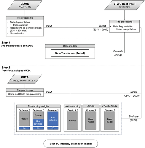
The overall flow of this study is illustrated in Figure 2. Our framework comprises the following two steps. In the first step, a pre-trained TC intensity estimation model based on a Swin Transformer (Swin-T) was built using COMS MI-based TC observations. In the second step, three transfer learning schemes based on the transfer level were investigated based on the best-performing pre-trained model using GK2A AMI-based observations. The best-performing and control models were compared to verify each model in TC intensity estimation. Details of the research framework are described in the following sections.

Figure 2. Overall flow chart of the proposed transfer learning-based tropical cyclone (TC) intensity estimation model.

3.1. Pre-processing of input datasets

According to the JTWC, 274 TCs occurred over the WNP between 2011 and 2021, yielding 14,199 scenes obtained from COMS MI and 4185 scenes obtained from GK2A AMI. Because the data for the entire lifetime of the TCs were utilized, the number of samples by intensity was imbalanced; there were too many samples for weak TCs and too few for strong TCs. Data imbalance leads to the overfitting of models to a group of large samples (Lee et al. 2020; Zhang et al. 2021). Data augmentation was conducted using the method proposed by Lee et al. (2020) to mitigate this problem. For data augmentation, the best track obtained every 6 hours was linearly interpolated for each hour. Subsequently, image-rotation-based augmentation was conducted at a 10 kt interval-wise frequency to augment the underrepresented data. The rotation angle was set between 30° and 180°, according to the number of augments required.

The images were cropped to a range of approximately 1200 × 1200 km (i.e. 301 × 301 pixels for COMS MI and 601 × 601 pixels for GK2A AMI) based on the TC center provided by the best tracks (Lee et al. 2020; Zhang, Liu, and Shi 2020) to cover the entire shape of the TCs. Subsequently, the COMS MI and GK2A AMI images were resampled to 5 km (224 × 224 pixels) to equalize the spatial resolution. Because the BT values derived from the IR channels exhibit diurnal and seasonal variability (Ba and Nicholson 1998; Norouzi et al. 2015), the values for each channel-wise scene were normalized from 0 to 1.

This study divided the datasets into training, validation, and test sets. The training and validation sets were used to train and optimize the deep learning models, respectively, and the test set was used to evaluate model performance. For Step 1 (base model), COMS MI-based TC observations from 2011 to 2017 were used to train and validate the models, whereas TC observations from 2018 were used to evaluate the base models. For Step 2 (transfer learning), GK2A AMI-based observations from September 2019 to December 2020 were used to fine-tune the weights of the pre-trained base model, whereas TC observations from 2021 were used to evaluate the performance of the transfer-learning-based models. The training and validation sets were randomly divided into 8:2 track-by-track sets and the data augmentation approach was applied only to the training sets. Table 2 summarizes the number of training, validation, and test sample images obtained using the model.

Table 2. Number of training, validation, and test samples for base and transfer models. Since the data augmentation approach was applied to only the training datasets, some outside and inside parentheses indicate the number of augmented and original samples, respectively.

Model	Dataset	Samples (original)
Base models	Train	55,941 (2768)
	Validation	568
	Test	861
Transfer learning models	Train	11,223 (371)
	Validation	88
	Test	632

3.2. Pre-training model using COMS MI

This study selected the Swin Transformer (Swin-T) as the base model to estimate the TC intensity. Unlike CNNs, which prioritize local image regions, transformers introduced in 2017 use self-attention to capture the global context (Vaswani et al. 2017; Ma et al. 2023). By relying on positional embedding and self-attention, transformers have a lower inductive bias than CNNs and require a large amount of training data for optimal performance. Swin-T was proposed to address the inherent challenges of applying transformers to local image characteristics (Liu et al. 2021). It adopts a multistage hierarchical design that calculates attention within distinct local windows and subdivides them into several sub-patches. Traditional multihead self-attention (MSA) is supplanted by shifted window-based multihead self-attention mechanisms (W-MSA/SW-MSA) to capture the interactions between different windows or image positions. The W-MSA and SW-MSA are used back and forth across each transformer layer, moving gradually along the network hierarchy to capture the overlapping areas. Recently, several studies have demonstrated the efficacy of Swin-T’s hierarchical design and shifted window methodology across various image recognition tasks, such as medical image classification and satellite image object segmentation (Gao et al. 2021; Liu et al. 2022; Yu et al. 2022; Ma et al. 2023; Xiao et al. 2023). Swin Ts are divided into T, S, B, and L versions based on the model size and computational complexity (Liu et al. 2021). A miniature version of the Swin-T family was used for modeling.

For pre-training using COMS MI, all layers of Swin-T were initialized with ImageNet’s pre-trained weights but were retrained on COMS MI-based TC observations. Swin-T was trained to minimize mean absolute error (MAE) with the Adam optimizer, using β1 = 0.9 and β2 = 0.999, with a weight decay of 0.01 and batch size of 64. In addition, the cosine annealing warm restart learning rate schedule was employed with a learning rate of 1e-5; the number of iterations for the first restart was 20, and the restart interval doubled afterward.

3.3. Transfer learning to GK2A

Three schemes (Schemes 1–3) were evaluated using GK2A to investigate the optimal transfer learning approach for TC intensity estimation. Scheme 1 conducts fine-tuning only for the last fully connected (FC) layer, Scheme 2 conducts fine-tuning for the last several stages of the network, and the FC layer, and Scheme 3 fine-tunes the entire pre-trained network (Figure 2). This stage indicates blocks with the same feature map size for each model. For Scheme 2, three sub-schemes were established by freezing the weight until the last, second, and third stages (Schemes 2–1, 2–2, and 2–3). The best-performing scheme was compared with control models to evaluate the efficacy of transfer learning. The three control models are defined as follows: Control 1 is a model that was pre-trained using COMS MI and then used without any further fine-tuning. Controls 2 and 3 did not involve transfer learning processes and maintained the base model structure while varying the input data. Specifically, Control 2 was trained solely using data from GK2A AMI, whereas Control 3 was trained using a combination of COMS MI and GK2A AMI data.

The transfer models’ learning rate was set to 1e-6, which was slower than during pre-training, to mitigate overfitting to the newly adopted samples. The batch size was set to 16, and a learning rate scheduler was not used. The remaining hyperparameter settings were the same as those used in previous COMS MI-based base models.

3.4. Accuracy assessment

To evaluate the performance of both the pre-trained and transfer learning models, the coefficient of determination (R², unitless), MAE (kts), root mean squared error (RMSE, kts), and relative root mean squared error (rRMSE, %) were used.

(1) $R^2=\frac{{\sum }_i^N\left(y_i-{\bar{y}}_{\mathit{i}}\right)\left({\hat{y}}_{\mathit{i}}-{\overline{\stackrel{ˆ}{y}}}_{\mathit{i}}\right)}{\sqrt{{\sum }_i^N{\left(y_i-{\bar{y}}_{\mathit{i}}\right)}^2{\sum }_i^N{\left({\hat{y}}_{\mathit{i}}-{\overline{\stackrel{ˆ}{y}}}_{\mathit{i}}\right)}^2}}$(1)

(2) $\mathit{MAE}=\frac{{\sum }_i^N\left|y_i-{\hat{y}}_{\mathit{i}}\right|}{\mathit{N}}$(2)

(3) $\mathit{RMSE}=\sqrt{\frac{{\sum }_i^N{\left(y_i-{\hat{y}}_{\mathit{i}}\right)}^2}{\mathit{N}}}$(3)

(4) $\mathit{rRMSE}=100\ast \frac{\sqrt{\frac{{\sum }_i^N{\left(y_i-{\hat{y}}_{\mathit{i}}\right)}^2}{\mathit{N}-1}}}{\bar{y}}$(4)

where ${\hat{y}}_{\mathit{i}}$, $y_i$ and $\bar{y}$ are the estimated, reference, and average intensities, respectively; $\mathit{N}$ is the total number of reference data points. In this study, the model-based TC intensity estimation was evaluated both entirely and intensity-wise. For intensity-wise evaluation of the models, the TCs were categorized according to the Saffir-Simpson criteria (Table 3).

Table 3. Tropical cyclone intensity based on Saffir Simpson category.

Category	Intensity (kts)
Tropical Depression (TD)	20–34
Tropical Storm (TS)	35–63
Category 1 (C1)	64–82
Category 2 (C2)	83–95
Category 3 (C3)	96–113
Category 4 (C4)	114–135
Category 5 (C5)	>135

The computational efficiency of the transfer learning performance was evaluated in addition to the statistical accuracy. This was achieved by measuring each scheme’s number of learnable parameters, memory usage, and computational time. The learnable parameters are those that the model updates during transfer learning. The evaluation was conducted using a single NVIDIA RTX 3090TI GPU with the GK2A input dataset set to 16 × 3 × 224 × 224 (batch size, channels, height, and width, respectively) to measure the GPU memory usage and time to train one epoch.

To further assess our model’s accuracy, we conducted a comparative analysis with the findings of previous studies. However, making an equivalent comparison is challenging because of variations in the datasets used by each study and differing definitions of TC intensity among meteorological agencies. For instance, the JTWC defines TC intensity based on the 1-minute maximum sustained wind speed, whereas the Japan Meteorological Agency and China Meteorological Administration use 10-minute and 2-minute maximum sustained wind speeds, respectively. The RMSE values for 10-minute and 2-minute maximum sustained wind speeds were adjusted by multiplying them by 1.14, as suggested by Powell et al. (1996) and Bai et al. (2022), to address these differences and provide a more consistent comparison.

4. Results and discussion

4.1. Pre-trained model performance

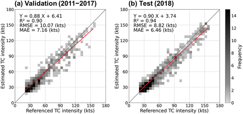
The base model, Swin-T, was quantitatively analyzed using two datasets: a validation set with 20% of TCs randomly selected by track from 2011 to 2017 and a test set of TCs in 2018 (Figure 3). The Swin-T-based TC intensity estimation achieved significant performance with an R² of 0.90 and an MAE of 7.16 kts for the validation set, and an R² of 0.94 and an MAE of 6.46 kts for the test set. However, as shown in the scatter plots of Figure 3a,b, Swin-T tended to slightly underestimate TC intensities exceeding 90 knots.

Figure 3. Validation and test results for tropical cyclone intensity estimation using the base model (i.e. Swin-T). The solid red line is the best-fit line derived using the least-square method.

Table 4 lists the error metrics for the validation and test sets of the base model, categorized by TC intensity. A prominent trend was observed, indicating that the relative error decreased as the intensity of the TC increased. In the Tropical Depression (TD) phase, with intensities below 34 knots, the Swin-T model recorded the highest rRMSE values: 30.47% for the validation set and 23.00% for the test set. However, it is important to note that, in absolute terms, the error was the smallest (with an MAE of 5.27 kts and RMSE of 7.38 kts for the validation set and MAE of 4.48 kts and RMSE of 5.80 kts for the test set). Conversely, for strong TCs exceeding 135 knots (C5), the Swin-T model showed the lowest relative error, with rRMSE of 12.32% for the validation set and 6.72% for the test set, whereas the absolute errors were comparable to those across all categories (MAE of 7.74 kts and RMSE of 9.79 kts). This demonstrates the ability of the model to accurately capture not only the subtleties of the initial developmental stage but also extremely highly intensified TCs, which are often the most destructive. Maintaining this level of accuracy is required after the implementation of transfer learning.

Table 4. Categorical model evaluation results of the base model (i.e. Swin-T) for tropical cyclones 2011–2018. The metrics with the lowest error in each category are highlighted in bold.

	Validation								Test
category	TD	TS	C1	C2	C3	C4	C5	Overall	TD	TS	C1	C2	C3	C4	C5	Overall
N	193	198	63	37	41	29	7	568	334	274	77	63	29	43	41	861
MAE (kts)	5.27	6.08	10.04	9.47	11.20	10.85	12.61	7.16	4.48	5.74	9.80	9.37	12.87	10.63	7.74	6.46
RMSE (kts)	7.38	7.88	12.70	13.19	14.96	15.30	18.03	10.07	5.80	7.25	12.33	12.25	16.91	13.66	9.79	8.82
rRMSE (%)	30.47	17.61	17.89	14.72	14.40	12.51	12.32	18.98	23.00	16.50	16.98	13.65	16.27	10.93	6.72	16.49

4.2. Transfer learning-based TC intensity estimation: COMS2GK2A

4.2.1. Transfer learning on GK2A

The optimal transfer learning method for the TC intensity estimation was investigated by varying the number of layers transferred from COMS to GK2A. Table 5 summarizes the evaluation results of the three Swin-T-based transfer-learning approaches (Schemes 1, 2, and 3). Scheme 1 (fine-tuning only for the FC layer) exhibited the lowest validation loss, but its performance degraded significantly on the test set (MAE of 6.45 kts for the validation set; MAE of 9.75 kts for the test set). This implies that fine-tuning only the FC layer is insufficient to optimize and generalize the GK2A-based observations. Scheme 2–1 (additional fine-tuning for the last stage) shows an MAE of 7.06 kts, achieving a significant improvement of 27.59% for the test set compared with Scheme 1. For Schemes 2–2 and 2–3, the performances improve according to the increases of fine-tuned stages, with MAEs of 6.62 kts and 6.53 kts, respectively. For the test set, Scheme 3 (fine-tuning for all layers) exhibited the highest performance (MAE of 6.48 kts). Compared to Scheme 1, the MAE improved by 33.54%, respectively.

Table 5. Overall validation and test results of transfer learning experiments with GEO-KOMPSAT-2A advanced meteorological imager. The stage represents a set of blocks in the Swin-T with the exact output resolution. The best-performing scheme model is shown in bold.

Scheme	Method	Validation			Test
		R^2	RMSE (kts)	MAE (kts)	R^2	RMSE (kts)	MAE (kts)
Scheme 1	Fine-tune FC layer	0.94	8.29	6.45	0.82	12.63	9.75
Scheme 2–1	Fine-tune Last 1 stage + FC layer	0.93	8.92	7.07	0.90	9.34	7.06
Scheme 2–2	Fine-tune Last 2 stage + FC layer	0.93	9.21	7.17	0.92	8.71	6.62
Scheme 2–3	Fine-tune Last 3 stage + FC layer	0.93	9.09	7.05	0.92	8.59	6.53
Scheme 3	Fine-tune all layers	0.93	8.95	6.90	0.92	8.50	6.48

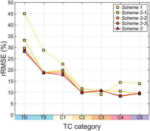
Figure 4 compares the rRMSEs for each intensity level using this scheme. In most TC categories, as the number of schemes increased (i.e. from Scheme 1 to Scheme 3), the performance of each scheme improved. The improvement was especially significant for categories TD and TS, where Scheme 3 reduced rRMSE by over 10%p compared to Scheme 1. Moreover, for strong TCs in categories C4 and C5, Scheme 3 also exhibited a notable decrease in rRMSE by approximately 5%p. Interestingly, the model performance improved consistently for both the overall and categorical evaluations as the number of fine-tuned layers increased. This is consistent with research in computer vision science, where fine-tuning all the layers is better than fixing the feature layers (Azizpour et al. 2015; Chu et al. 2016; Huh et al. 2016; Kornblith et al. 2019). Utilizing only past sensor information with similar spectral wavelengths will not improve the performance owing to the differences in specifications and sensitivity between sensors. Therefore, it is necessary to fine-tune all model layers to adjust for the differences between the satellite sensor channels. It was also demonstrated that after applying transfer learning, the Scheme 3 model maintained a high level of accuracy, similar to the pre-trained model.

Figure 4. Relative root mean squared errors (rRMSE) across the Saffir Simpson category of TC intensity tropical cyclone (TC) intensity for the five transfer learning scheme models (i.e. Scheme 1, Scheme 2–1–2–3, and Scheme 3) using GEO-KOMPSAT-2A advanced meteorological imager for the 2021 test set.

The computational efficiency of each scheme was evaluated by calculating the number of training parameters, memory usage, and training time per epoch (Table 6). The results revealed a substantial difference in the number of learnable parameters between Scheme 1 (769) and Scheme 3 (27.52 million), as well as a variation in memory usage (Scheme 1:2560 MiB and Scheme 3:4212 MiB). Including more fixed layers can decrease memory usage because they are not included in gradient storage and computation during backpropagation. However, the training time per epoch ranged from 52 s to 61 s, with Scheme 1 and 3 differing by only 9 s. Thus, although Scheme 1 and 3 differ in the number of parameters and memory usage, the minimal difference in the training time suggests that both schemes offer comparable computational efficiency.

Table 6. Comparison of the computational efficiency of Swin-T transfer learning schemes for the GEO-KOMPSAT-2A advanced meteorological imager tropical cyclone observations. The memory usage indicates the memory occupied during training when the batch size is 16, and the training time represents the duration of a single epoch using an NVIDIA RTX 3090Ti GPU.

Scheme	Scheme 1	Scheme 2–1	Scheme 2–2	Scheme 2–3	Scheme 3
Learnable parameters (M: millions)	769	14.19 M	26.03 M	27.22 M	27.52 M
Memory usage (MiB)	2560	2644	3068	3510	4212
training time per one epoch (s)	52	54	54	56	61

4.2.2. Comparison with control models

To evaluate the efficacy of transfer learning, Scheme 3 was compared with three control models: a COMS MI-based pre-trained base model without fine-tuning with GK2A AMI (Control 1), a base model trained using only GK2A AMI (Control 2), and a base model trained using COMS MI and GK2A AMI observations (Control 3). Figure 5 shows scatter plots of the test results for the control and transfer learning models (Scheme 3). Scheme 3 yielded the highest accuracy, with an MAE of 6.48 kts (Figure 5(d)), followed by Control 3 (MAE = 7.02 kt) (Figure 5(c)), Control 2 (MAE = 7.82 kt) (Figure 5(b)), and Control 1 (MAE = 13.74 kt) (Figure 5(a)). The best-fit line of Scheme 3 correlated at y = 0.95× + 3.33 (R²:0.92), and the existing outliers were significantly reduced. Control 1 tends to overestimate weak TC intensities and underestimate strong TC intensities (Figure 5(a)). This implies that the information learned from COMS alone is unsuitable for direct application to the intensity estimation model for GK2A. Control 2, trained solely on GK2A data, performed better than Control 1. However, owing to the limited amount of training data, there is a limitation in improving accuracy, especially for strong TCs with a small number of samples. Compared to Control 2, Control 3, which was trained with more samples by combining COMS and GK2A, showed better performance. This indicated that increasing the sample size could improve the model’s performance. Nonetheless, the transfer learning approach yielded the best performance. In particular, for TC intensities greater than 120 kts, Scheme 3 exhibited a significant reduction in error compared to Control 3.

Figure 5. Density scatterplots of test results for the three control and proposed transfer learning models. (a)–(c) indicates Controls 1–3, respectively, and (d) indicates Scheme 3. The x-axis and y-axis imply the Joint Typhoon Warning Center’s best track-based and the estimated tropical cyclone intensities (unit: kts) for each model, respectively.

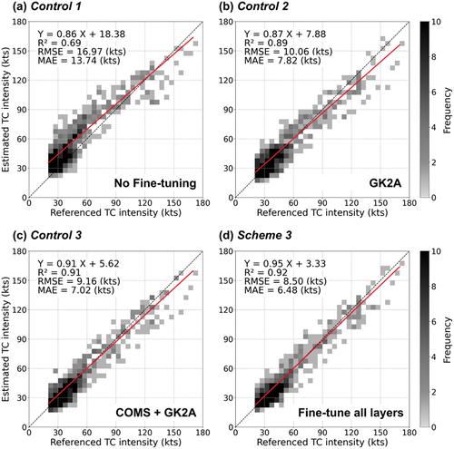
Table 7 summarizes the accuracy metrics for the control models and Scheme 3 based on the TC intensity. Scheme 3 exhibited the highest accuracy in most intensity categories, with better performance at low and high intensities than the control models. Control 2 had the most minor error for C1, and Control 1 had the most significant error for the same category. The difference between COMS and GK2A information was most pronounced in C1. After transfer learning, Scheme 3 significantly reduced the error for the C1 category, but still had a slightly larger error than Control 2. For C3, Control 3 outperformed Scheme 3. Exceptionally, the performance was worse even when transfer learning was conducted using the GK2A data (Scheme 3). However, the transfer learning model exhibited significant performance improvement in the remaining categories.

Table 7. Intensity-wise model evaluation results of proposed transfer learning-based model (Scheme 3) and control models using tropical cyclones (TCs) in 2021. The metrics with the lowest error in each category are shown in bold.

Scheme	Method	TC category	TD	TS	C1	C2	C3	C4	C5	Overall
		N	251	253	42	26	16	33	11	632
Control 1	No Fine-tuning in COMS pre-trained model	MAE	13.50	14.07	18.43	9.93	8.82	11.95	15.20	13.74
		RMSE	16.83	17.26	20.86	12.73	10.26	15.00	18.78	16.97
		rRMSE	44.02	30.90	23.62	12.74	9.23	12.83	13.70	35.87
Control 2	GK2A	MAE	6.65	7.75	9.00	8.59	10.12	11.07	16.42	7.82
		RMSE	8.69	9.49	10.90	10.43	13.34	14.24	21.04	10.06
		rRMSE	29.13	21.24	14.78	11.85	13.57	12.49	15.16	21.27
Control 3	COMS + GK2A	MAE	5.86	6.72	9.21	9.29	8.17	10.40	14.62	7.02
		RMSE	8.00	8.25	10.93	11.50	10.57	12.82	19.25	9.16
		rRMSE	27.84	18.91	15.05	12.94	10.13	10.94	13.82	19.37
Scheme 3	Fine-tuning all layers	MAE	5.25	6.41	10.06	6.45	9.29	8.21	13.04	6.48
		RMSE	7.05	8.07	12.61	9.10	11.35	10.25	14.82	8.50
		rRMSE	25.13	19.14	17.03	10.10	10.66	8.66	10.17	17.98

The four previous studies that combined data from multiple sensors in a manner similar to Control 3 are summarized in Table 8. They collected all TC images from the Himawari satellite series and used them as the same input features without any specific processing of the different sensor data. Despite gathering extensive long-term sample data, Combinido et al. (2018), Jiang and Tao (2022), and Zhang et al. (2021) achieved significantly lower accuracy because of their reliance on single-channel images. Jiang et al. (2023) estimated TC intensity using four channels under conditions similar to Control 3, resulting in comparable accuracy. In contrast, Scheme 3 exhibited superior performance despite the relatively short-term training data. This indicates that transfer learning enables the model to be more effectively optimized for the currently operating satellite sensor while utilizing all available data for more accurate TC intensity estimation. This finding also suggests that the algorithms developed for previous satellite missions can be used to enhance their accuracy by reoptimizing newly generated satellite missions.

Table 8. Comparison with previous studies using the multiple satellite sensors-based tropical cyclone intensity estimation approaches. The metrics with the lowest error are shown in bold.

Model	Dataset	Channel	Covered period	Test period	RMSE	Reference
VGG19	GMS5, GEOS-9, MTSAT-1R, MTSAT-2, and Himawari 8	Single IR	1996 to 2016	2015, 2016	15.08 kts	Combinido et al. (2018)
TICAENet	GMS5, GEOS-9, MTSAT-1R, MTSAT-2, and Himawari 8	Single IR	1995 to 2020	Random split	13.54 kts	Jiang and Tao (2022)
TCICENet-S	GMS1–5, GEOS-9, MTSAT-1R, MTSAT-2, and Himawari 8	Single IR	1981 to 2019	2017 to 2019	9.80 kts	Zhang et al. (2021)
DMANet_KF	MTSAT-1R, MTSAT-2, and Himawari 8	4 IR channels	2007 to 2021	Random split	8.91 kts	Jiang et al. (2023)
Swin Transformer (Control 3, non-transfer learning)	COMS, GK2A	3 IR channels	2011 to 2021	2021	9.16 kts	This study
Swin Transformer (Scheme 3, Transfer learning)	COMS, GK2A	3 IR channels	2011 to 2021	2021	8.50 kts

4.3. Time-series evaluation of TCs in 2021

To examine the model performance for the entire TC lifetime, four strong TCs were considered for 2021 (Typhoons Surigae, Mindulle, Nyatoh, and Rai). Figure 6 shows the time series of the intensity estimation results for the four TCs using Scheme 3 and Control Models 1–3. Scheme 3 exhibits the most robust performance for all cases compared to the control models. Control 1 showed an overestimation of the TC development phase (e.g. from 4 November 2021 18:00 UTC to 04/16/2021 06:00 UTC in Typhoon Surigae and from 09/22/2021 12:00 to 09/25/2021 00:00 UTC in Typhoon Mindulle). Controls 2 and 3 underestimated the rapid intensification from 04/17/2021 00:00 UTC on 04/17/2021 to 12:00 UTC. Scheme 3 in Figure 6(a) shows a better estimation of the maximum TC intensity of Typhoon Surigae at 04/17/2021 12:00 UTC than other scheme-based estimations. However, it overestimated the weak intensities (C1 cases) and underestimated them at 04/18/2021 00:00 and 06:00 UTC after the TC peak. This underestimation was also observed in a study by Zhang et al. (2022b), who utilized DenseConvMixer to estimate the intensity of Typhoon Surigae and showed a significant underestimation during the same period. Figure 6(c) shows Typhoon Nyatoh, which rapidly intensified offshore and dissipated into the open ocean – all models, except Control 1, produced results consistent with the JTWC best track. In contrast, in the case of Typhoon Rai (Figure 6(d)), all models showed significant variability in the estimates over the island (12/16/2021 at 12:00 UTC − 12/17/2021 at 00:00 UTC). Because of TC, the structural characteristics of landfall became disorganized during this period (Supplementary Fig S1). This caused an underestimation in all the image recognition models.

Figure 6. Time-series comparison of Scheme 3 and Controls 1, 2, and 3 with Joint Typhoon Warning Center best track data of Typhoon SURIGAE, MINDULLE, NYATOH, and RAI in 2021. The x-axis indicates the observation date (mm-dd hh: mn), and the y-axis indicates the tropical cyclone (TC) intensity (kts). The white and gray boxes represent the developing and dissipating phases, respectively.

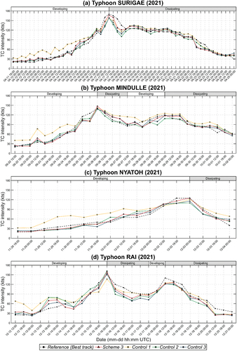
Overall, Scheme 3 shows a time series pattern to that of the JTWC but is sensitive to rapid changes in TC intensity. While the MAE for the entire lifetimes of the four TCs was 7.68 kts, it showed significant differences between developing and dissipating phases (MAE of 7.03 kts in developing phases and MAE of 8.87 kts in dissipating phases). Mainly, during the dissipation phase, changes such as the loss of the eye of the storm or the splitting of cloud bands made it difficult for the model to make an accurate estimation. The incorporation of temporal information may be useful to address this challenge.

4.4. Interpretability of deep learning-based TC intensity estimation model

Although there have been many attempts to analyze the features learned by CNN-based TC intensity estimation models (e.g. Lee et al. 2020; Wang et al. 2022), there has been no analysis of transformer-based TC intensity estimation models. To verify how the Swin-T model works in estimating intensity, an eigen-class activation map (Eigen-CAM)-based visualization was conducted and compared to the Dvorak-technique-based intensity-wise TC patterns (Figure 7). Eigen-CAM computes and visualizes the principal components of the learned features and representations from the layers (Muhammad and Yeasin 2020). In the last block of each stage, features were extracted from the attention layer and reshaped to form 2-dimensional spatial images, which allowed for visualization and analysis of the activations and gradients of the features.

Figure 7. Comparison of Dvorak technique-based TC patterns and eigen-CAM activation regions for each model stage according to TC category. TD is the infrared image of typhoon choi-wan (05/29/2021 06:00 UTC), TS is typhoon Konpasu (10/11/2021 12:00 UTC), C1 is typhoon In-fa (07/22/2021 12: 00 UTC), C2 is typhoon mindulle (C2: 09/27/2021 12:00 UTC), C3 is typhoon nyatoh (12/02/2021 12:00 UTC), C4 is typhoon surigae (04/18/2021 12:00 UTC) and C5 is typhoon Rai (12/16/2021 00:00 UTC).

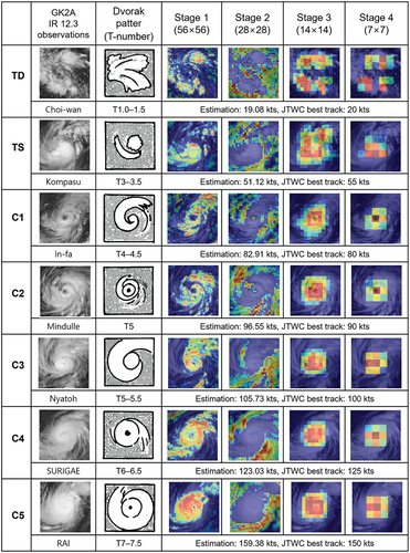
In Stage 1, the Swin-T model captures the overall shape of the TC. The activated maps exhibited similarities to the Dvorak pattern. This implies that the model successfully captures most of the intensity-related features of the TC. In Stage 2, the outer patterns of the TC were captured, with a specific emphasis on remote rainbands. There was no overlap with the regions activated in Stage 1, indicating that the Swin-T model focused on the remaining regions not activated in Stage 1. In Stage 3, the Swin-T model focuses on the cloud cluster region. For the TD, multiple clusters of the model were captured instead of just one. This implies that the Swin-T-based model successfully considers the inorganization of weak TC. After C1, the model concentrated on the spiral patterns around the eyewall. For C4 and C5, the activated features are focused on the TC eyewall. In Stage 4, the activated features became simpler: the stronger the TC intensity, the more focused on the central area. Interestingly, especially in TCs above the C1 category, it seems that the activated features represent more high-dimensional information as the level of the stage increases, from pattern recognition to intensity estimation.

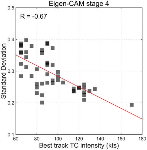
To verify that the stage 4-based feature was related to the intensity estimation value of TCs over the C1 category, the relationship between them was analyzed (Figure 8). Relationship between standard deviation (SD) of stage 4-based Eigen-CAM results and TC intensity. Here, to verify how the model works, only the well-estimated cases (≤ absolute error of 5 kts) were evaluated. As shown in Figure 8, there was a clear trend for the SD to decrease as the TC intensity increased (R = −0.67). The Eigen-CAM results for weak TCs exhibited a dispersed pattern, which can be attributed to the disorganized structure of the TCs. However, as TC strengthens, they tend to become increasingly organized. This implies that Swin-T can differentiate the intensity-dependent attributes of a TC with greater emphasis on the consistent features present in stronger TCs. As the eye developed, Swin-T was highly activated in all regions around the eye. In summary, the Swin-T model considers different TC aspects for each stage. However, as the layers deepened, the pattern at the center of the TC appeared to be the most important for estimating TC intensity.

Figure 8. Scatterplot of standard deviation of eigen-CAM result from stage 4. Zero values are excluded in calculating standard deviation. Samples were selected with a TC category of C1 or higher and an absolute error of 5 kts or less.

5. Conclusion

This study proposes a framework for transfer learning using an end-of-mission COMS-based TC intensity estimation model to enhance the current operational GK2A-based TC intensity estimation model. Swin-T was used as the base model, and the model pre-trained with COMS achieved an MAE of 6.46 kts. Transfer learning approaches were used to apply the model to GK2A. Our study revealed that the performance of transfer learning improved with an increasing number of fine-tuning layers: a method for fine-tuning all layers (Scheme 3) achieved an MAE of 6.48 kts, whereas a method for fine-tuning only the last layer (Scheme 1) yielded an MAE of 9.75 kts. Compared with the non-transfer learning models (i.e. Controls 1–3), the proposed transfer learning-based model (i.e. Scheme 3) achieved a 7–52% improvement in performance. Moreover, Eigen-CAM-based visualization demonstrated the validity of the transformer-based model for TC intensity estimation by verifying that the model considered various regions of a TC based on intensity, such as the overall shape, eyewalls, and eyes of the TC.

The transfer learning approach used in this study is straightforward yet highly effective. This approach is expected to benefit future TC intensity estimation studies, mainly when dealing with multi-satellite data. However, there is scope for further improvement. In this study, because only 80% of the two years’ TCs were utilized for training the transfer learning-based models, the number of dissipating weak TC samples was inevitably insufficient, which caused relatively poor performance for TCs in the dissipating phases. This is expected to improve as the training period for the GK2A increases.

Disclosure statement

No potential conflict of interest was reported by the author(s).

Data availability statement

The raw data used in this study are publicly available from the following sources: The processed data and code generated in this study are available upon request from the corresponding authors.

• COMS and GK2A satellite observations: https://nmsc.kma.go.kr/

• JTWC best track: https://www.metoc.navy.mil/jtwc/jtwc.html?best-tracks

• Source code of Swin-T: https://github.com/huggingface/pytorch-image-models

Correction Statement

This article has been republished with minor changes. These changes do not impact the academic content of the article.

Additional information

Funding

This research was supported by Korea Institute of Marine Science & Technology (KIMST) funded by the Ministry of Oceans and Fisheries (RS-2023-00256330, Development of risk managing technology tackling ocean and fisheries crisis around Korean Peninsula by Kuroshio Current) and by the MSIT (Ministry of Science and ICT), Korea, under the ITRC(Information Technology Research Center) support program (IITP-2023-2018-0-01424) supervised by the IITP(Institute for Information & communications Technology Promotion).

References

- Azizpour, H., A. S. Razavian, J. Sullivan, A. Maki, and S. Carlsson. 2015. “Factors of Transferability for a Generic Convent Representation.” IEEE Transactions on Pattern Analysis and Machine Intelligence 38 (9): 1790–18. https://doi.org/10.1109/TPAMI.2015.2500224.
- Bai, L., J. Tang, R. Guo, S. Zhang, and K. Liu. 2022. “Quantifying Interagency Differences in Intensity Estimations of Super Typhoon Lekima (2019).” Frontiers of Earth Science 16 (1): 1–12. https://doi.org/10.1007/s11707-020-0866-5.
- Ba, M. B., and S. E. Nicholson. 1998. “Analysis of Convective Activity and Its Relationship to the Rainfall Over the Rift Valley Lakes of East Africa During 1983–90 Using the Meteosat Infrared Channel.” Journal of Applied Meteorology 37 (10): 1250–1264. https://doi.org/10.1175/1520-0450(1998)037<1250:AOCAAI>2.0.CO;2.
- Chang, F. L., and Z. Li. 2003. “Retrieving vertical profiles of water‐cloud droplet effective radius: Algorithm modification and preliminary application.” Journal of Geophysical Research: Atmospheres 108 (D24). https://doi.org/10.1029/2003JD003906.
- Chu, B., V. Madhavan, O. Beijbom, J. Hoffman, and T. Darrell. 2016. Best Practices for Fine-Tuning Visual Classifiers to New Domains. In Computer Vision–ECCV 2016 Workshops: Amsterdam, The Netherlands, October 8–10 and 15–16, 2016, Proceedings, Part III 14, Amsterdam, The Netehrlands, 435–442. Springer International Publishing.
- Combinido, J. S., J. R. Mendoza, and J. Aborot. 2018. “A Convolutional Neural Network Approach for Estimating Tropical Cyclone Intensity Using Satellite-Based Infrared Images.” In 2018 24th International conference on pattern recognition (ICPR), Beijing, China, 1474–1480. IEEE.
- Combinido, J. S., J. R. Mendoza, and J. Aborot. (2018, August). ”A Convolutional Neural Network Approach for Estimating Tropical Cyclone Intensity Using Satellite-Based Infrared Images.” In 2018 24th International conference on pattern recognition (ICPR), 1474–1480. Beijing, China. IEEE.
- Dvorak, V. F. 1975. “Tropical Cyclone Intensity Analysis and Forecasting from Satellite Imagery.” Monthly Weather Review 103 (5): 420–430. https://doi.org/10.1175/1520-0493(1975)103<0420:TCIAAF>2.0.CO;2.
- Gadiraju, K. K., and R. R. Vatsavai. 2023. “Application of Transfer Learning in Remote Sensing Crop Image Classification.” IEEE Journal of Selected Topics in Applied Earth Observations and Remote Sensing 16: 4699–4712.
- Gao, L., H. Liu, M. Yang, L. Chen, Y. Wan, Z. Xiao, and Y. Qian. 2021. “STransFuse: Fusing Swin Transformer and Convolutional Neural Network for Remote Sensing Image Semantic Segmentation.” In IEEE Journal of Selected Topics in Applied Earth Observations and Remote Sensing 14:10990–11003. https://doi.org/10.1109/JSTARS.2021.3119654.
- Gao, S., L. Zhu, W. Zhang, and X. Shen. 2020. “Western North Pacific Tropical Cyclone Activity in 2018: A Season of Extremes.” Scientific Reports 10 (1): 1–9. https://doi.org/10.1038/s41598-020-62632-5.
- Gomroki, M., M. Hasanlou, and P. Reinartz. 2023. “STCD-EffV2T Unet: Semi Transfer Learning EfficientNetv2 T-Unet Network for Urban/Land Cover Change Detection Using Sentinel-2 Satellite Images.” Remote Sensing 15 (5): 1232. https://doi.org/10.3390/rs15051232.
- Guo, X., J. Yin, and J. Yang. 2024. ”Fine classification of crops based on an inductive transfer learning method with compact polarimetric SAR images.” GIScience & Remote Sensing 61 (1). https://doi.org/10.1080/15481603.2024.2319939.
- Hewison, T. J., X. Wu, F. Yu, Y. Tahara, X. Hu, D. Kim, and M. Koenig. 2013. “GSICS Inter-Calibration of Infrared Channels of Geostationary Imagers Using Metop/IASI.” IEEE Transactions on Geoscience and Remote Sensing 51 (3): 1160–1170. https://doi.org/10.1109/TGRS.2013.2238544.
- Huh, M., P. Agrawal, and A. A. Efros. 2016. “What Makes ImageNet Good for Transfer Learning?” arXiv preprint arXiv:1608.08614.
- Iman, M., H. R. Arabnia, and K. Rasheed. 2023. “A review of deep transfer learning and recent advancements.” Technologies 11 (2): 40. https://doi.org/10.3390/technologies11020040.
- Jiang, W., G. Hu, T. Wu, L. Liu, B. Kim, Y. Xiao, and Z. Duan. 2023. “DMANet_KF: Tropical Cyclone Intensity Estimation Based on Deep Learning and Kalman Filter from Multi-Spectral Infrared Images.” IEEE Journal of Selected Topics in Applied Earth Observations and Remote Sensing 16: 4469–4483.
- Jiang, S., and L. Tao. 2022. “Classification and Estimation of Typhoon Intensity from Geostationary Meteorological Satellite Images Based on Deep Learning.” Atmosphere 13 (7): 1113. https://doi.org/10.3390/atmos13071113.
- Kaur, S., S. Gupta, S. Singh, V. T. Hoang, S. Almakdi, T. Alelyani, and A. Shaikh. 2022. “Transfer Learning-based Automatic Hurricane Damage Detection Using Satellite Images.” Electronics 11 (9): 1448. https://doi.org/10.3390/electronics11091448.
- Kim, D. H., and M. H. Ahn. 2014. “Introduction of the In-Orbit Test and Its Performance for the First Meteorological Imager of the Communication, Ocean, and Meteorological Satellite.” Atmospheric Measurement Techniques 7 (8): 2471–2485. https://doi.org/10.5194/amt-7-2471-2014.
- Kim, D., M. H. Ahn, and M. Choi. 2015. “Inter-Comparison of the Infrared Channels of the Meteorological Imager Onboard COMS and Hyperspectral IASI Data.” Advances in Atmospheric Sciences 32 (7): 979–990. https://doi.org/10.1007/s00376-014-4124-1.
- Kim, D., M. Gu, T. H. Oh, E. K. Kim, and H. J. Yang. 2021. “Introduction of the Advanced Meteorological Imager of Geo-Kompsat-2a: In-Orbit Tests and Performance Validation.” Remote Sensing 13 (7): 1303. https://doi.org/10.3390/rs13071303.
- Knapp, K. R., M. C. Kruk, D. H. Levinson, H. J. Diamond, and C. J. Neumann. 2010. “The International Best Track Archive for Climate Stewardship (IBTrAcs) Unifying Tropical Cyclone Data.” Bulletin of the American Meteorological Society 91 (3): 363–376. https://doi.org/10.1175/2009BAMS2755.1.
- Kornblith, S., J. Shlens, and Q. V. Le. 2019. “Do Better Imagenet Models Transfer Better?.” In Proceedings of the IEEE/CVF conference on computer vision and pattern recognition, California, USA, 2661–2671.
- Krichene, H., T. Vogt, F. Piontek, T. Geiger, C. Schötz, and C. Otto. 2023. “The Social Costs of Tropical Cyclones.” Nature Communications 14 (1): 7294. https://doi.org/10.1038/s41467-023-43114-4.
- Kurniawan, A. A., K. Usman, and R. Y. N. Fuadah. 2019, November. “Classification of Tropical Cyclone Intensity on Satellite Infrared Imagery Using SVM Method.” In 2019 IEEE Asia Pacific Conference on Wireless and Mobile (APWiMob), Bali, Indonesia, 69–73. IEEE.
- Lee, S., and J. Choi. 2022. “A Snow Cover Mapping Algorithm Based on a Multitemporal Dataset for GK-2A Imagery.” GIScience & Remote Sensing 59 (1): 1078–1102. https://doi.org/10.1080/15481603.2022.2097395.
- Lee, J., J. Im, D. H. Cha, H. Park, and S. Sim. 2020. “Tropical Cyclone Intensity Estimation Using Multi-dimensional Convolutional Neural Networks From Geostationary Satellite Data.” Remote Sensing 12 (1): 108. https://doi.org/10.3390/rs12010108.
- Lee, J., M. Kim, J. Im, H. Han, and D. Han. 2021. ”Pre-trained feature aggregated deep learning-based monitoring of overshooting tops using multi-spectral channels of GeoKompsat-2A advanced meteorological imagery.” GIScience & Remote Sensing 58 (7): 1052–1071. https://doi.org/10.1080/15481603.2021.1960075.
- Liu, Z., Y. Lin, Y. Cao, H. Hu, Y. Wei, Z. Zhang, and B. Guo. 2021. “Swin Transformer: Hierarchical Vision Transformer Using Shifted Windows.” In Proceedings of the IEEE/CVF international conference on computer vision, Montreal, Canada, 10012–10022.
- Liu, Z., J. Ning, Y. Cao, Y. Wei, Z. Zhang, S. Lin, and H. Hu. 2022. “Video swin transformer.” In Proceedings of the IEEE/CVF conference on computer vision and pattern recognition, New Orleans, USA, 3202–3211.
- Lv, Z., K. Nunez, E. Brewer, and D. Runfola. 2024. ”Mapping the tidal marshes of coastal Virginia: a hierarchical transfer learning approach.” GIScience & Remote Sensing 61 (1). https://doi.org/10.1080/15481603.2023.2287291.
- Magee, A. D., D. C. Verdon-Kidd, and A. S. Kiem. 2016. “An Intercomparison of Tropical Cyclone Best-Track Products for the Southwest Pacific.” Natural Hazards and Earth System Sciences 16 (6): 1431–1447. https://doi.org/10.5194/nhess-16-1431-2016.
- Ma, D., L. Jiang, J. Li, and Y. Shi. 2023. “Water Index and Swin Transformer Ensemble (WISTE) for Water Body Extraction from Multi-Spectral Remote Sensing Images.” GIScience & Remote Sensing 60 (1): 2251704. https://doi.org/10.1080/15481603.2023.2251704.
- Ma, D., L. Jiang, J. Li, and Y. Shi. 2023. ”Water index and Swin Transformer Ensemble (WISTE) for water body extraction from multispectral remote sensing images.” GIScience & Remote Sensing 60 (1). https://doi.org/10.1080/15481603.2023.2251704.
- Muhammad, M. B., and M. Yeasin. 2020. “Eigen-Cam: Class Activation Map Using Principal Components.” In 2020 international joint conference on neural networks (IJCNN), Glasgow, UK, July, 1–7. IEEE.
- Norouzi, H., M. Temimi, A. AghaKouchak, M. Azarderakhsh, R. Khanbilvardi, G. Shields, and K. Tesfagiorgis. 2015. “Inferring Land Surface Parameters from the Diurnal Variability of Microwave and Infrared Temperatures.” Physics and Chemistry of the Earth, Parts A/B/C 83:28–35. https://doi.org/10.1016/j.pce.2015.01.007.
- Olander, T. L., and C. S.Velden. 2007. ”The Advanced Dvorak Technique: Continued Development of an Objective Scheme to Estimate Tropical Cyclone Intensity Using Geostationary Infrared Satellite Imagery.” Weather and Forecasting 22 (2): 287–298. https://doi.org/10.1175/WAF975.1.
- Piñeros, M. F., E. A. Ritchie, and J. S. Tyo. 2011. ”Estimating Tropical Cyclone Intensity from Infrared Image Data.” Weather and Forecasting 26 (5): 690–698. https://doi.org/10.1175/WAF-D-10-05062.1.
- Powell, M. D., S. H. Houston, and T. A. Reinhold. 1996. “Hurricane Andrew’s Landfall in South Florida. Part I: Standardizing Measurements for Documentation of Surface Wind Fields.” Weather and Forecasting 11 (3): 304–328. https://doi.org/10.1175/1520-0434(1996)011<0304:HALISF>2.0.CO;2.
- Pradhan, R., R. S. Aygun, M. Maskey, R. Ramachandran, and D. J. Cecil. 2018. “Tropical Cyclone Intensity Estimation Using a Deep Convolutional Neural Network.” IEEE Transactions on Image Processing 27 (2): 692–702. https://doi.org/10.1109/TIP.2017.2766358.
- Ritchie, E. A., G. Valliere-Kelley, M. F. Piñeros, and J. S. Tyo. 2012. ”Tropical Cyclone Intensity Estimation in the North Atlantic Basin Using an Improved Deviation Angle Variance Technique.” Weather and Forecasting 27 (5): 1264–1277. https://doi.org/10.1175/WAF-D-11-00156.1.
- Schreck, C. J., III, K. R. Knapp, and J. P. Kossin. 2014. “The Impact of Best Track Discrepancies on Global Tropical Cyclone Climatologies Using IbtrACS.” Monthly Weather Review 142 (10): 3881–3899. https://doi.org/10.1175/MWR-D-14-00021.1.
- Vaswani, A., N. Shazeer, N. Parmar, J. Uszkoreit, L. Jones, A. N. Gomez, and I. Polosukhin. 2017. “Attention is All You Need.” In proceedings of the 2017 Conference on Advances in Neural Information Processing Systems, Long Beach, CA, USA, 4–9 December 2017. 5998–6008.
- Wang, C., G. Zheng, X. Li, Q. Xu, B. Liu, and J. Zhang. 2022. “Tropical Cyclone Intensity Estimation from Geostationary Satellite Imagery Using Deep Convolutional Neural Networks.” IEEE Transactions on Geoscience and Remote Sensing 60: 1–16. https://doi.org/10.1109/TGRS.2021.3066299.
- Weiss, K., T. M. Khoshgoftaar, and D. Wang. 2016. “A Survey of Transfer Learning.” Journal of Big Data 3 (1): 1–40. https://doi.org/10.1186/s40537-016-0043-6.
- Wu, X., T. Hewison, and Y. Tahara. 2009. ”GSICS GEO-LEO intercalibration: Baseline algorithm and early results.” In proceedings of theAtmospheric and Environmental Remote Sensing Data Processing and Utilization V: Readiness for GEOSS III, San Diego, CA, USA, 2–6 August 2009, Vol. 7456, 25–36. Bellingham, WA, USA: SPIE.
- Xiao, H., L. Li, Q. Liu, X. Zhu, and Q. Zhang. 2023. ”Transformers in medical image segmentation: A review.” Biomedical Signal Processing and Control 84: 104791. https://doi.org/10.1016/j.bspc.2023.104791.
- Ye, R., and Q. Dai. 2021. “Implementing Transfer Learning Across Different Datasets for Time Series Forecasting.” Pattern Recognition 109: 107617. https://doi.org/10.1016/j.patcog.2020.107617.
- Yin, G., J. Baik, and J. Park. 2022. “Comprehensive Analysis of GEO-KOMPSAT-2A and FengYun Satellite-Based Precipitation Estimates Across Northeast Asia.” GIScience & Remote Sensing 59 (1): 782–800. https://doi.org/10.1080/15481603.2022.2067970.
- Yu, B., F. Chen, N. Wang, L. Yang, H. Yang, and L. Wang. 2022. ”MSFTrans: a multi-task frequency-spatial learning transformer for building extraction from high spatial resolution remote sensing images.” GIScience & Remote Sensing 59 (1): 1978–1996. https://doi.org/10.1080/15481603.2022.2143678.
- Zhang, D., Z. Liu, and X. Shi. 2020, December. “Transfer Learning on Efficientnet for Remote Sensing Image Classification.” In 2020 5th International Conference on Mechanical, Control and Computer Engineering (ICMCCE), Harbin, China, 2255–2258. IEEE.
- Zhang, M., H. Singh, L. Chok, and R. Chunara. 2022. “Segmenting Across Places: The Need for Fair Transfer Learning with Satellite Imagery.” In Proceedings of the IEEE/CVF Conference on Computer Vision and Pattern Recognition, New Orleans, USA, 2916–2925.
- Zhang, Y., and B. Wallace. 2015. “A Sensitivity Analysis of (And practitioners’ Guide To) Convolutional Neural Networks for Sentence Classification.” arXiv Preprint arXiv 1510:03820.
- Zhang, C. J., X. J. Wang, L. M. Ma, and X. Q. Lu. 2021. “Tropical Cyclone Intensity Classification and Estimation Using Infrared Satellite Images with Deep Learning.” In IEEE Journal of Selected Topics in Applied Earth Observations and Remote Sensing 14: 2070–2086. https://doi.org/10.1109/JSTARS.2021.3050767.
- Zhang, Z., X. Yang, X. Wang, B. Wang, C. Wang, and Z. Du. 2022. “A Neural Network with Spatiotemporal Encoding Module for Tropical Cyclone Intensity Estimation from Infrared Satellite Image.” Knowledge-Based Systems 258:110005. https://doi.org/10.1016/j.knosys.2022.110005.
- Zhuang, F., Z. Qi, K. Duan, D. Xi, Y. Zhu, H. Zhu, and Q. He, Q. He. 2021. “A Comprehensive Survey on Transfer Learning.” Proceedings of the IEEE 109 (1): 43–76. https://doi.org/10.1109/JPROC.2020.3004555.