A novel spaceborne photon-counting laser altimeter denoising method based on parameter-adaptive density clustering

ABSTRACT

To tackle the challenge of denoising spaceborne photon-counting laser altimeter point clouds with uneven noise density, this study proposes a denoising method based on adaptive parameter density clustering, which utilizes numerical simulations to achieve self-adaptation of key parameters (neighborhood radius $\mathit{Eps}$ and minimum number of points $\mathit{MinPts}$). First, taking the directional adaptive ellipse DBSCAN (DAE-DBSCAN) as an example, photons with different background photon count rates ($\mathit{bckgrd}\_\mathit{rate}$) are used to traverse $\mathit{Eps}$ and $\mathit{MinPts}$ to calculate their optimal values ($\mathit{Eps}$ and $\mathit{MinPts}$ with the highest denoising accuracy). Then, a mathematical prediction model of $\mathit{bckgrd}\_\mathit{rate}$, $\mathit{Eps}$ and $\mathit{MinPts}$ was established. The actual background photon count rates were introduced into the key parameter prediction model to obtain the optimal $\mathit{Eps}$ and $\mathit{MinPts}$. Finally, a denoising experiment was conducted using the simulated photons and the ATLAS data. The results show that the proposed method had higher accuracy than the constant parameter denoising method, with an $\mathit{F}$ >0.95. Even for photons of complex mountainous terrain with a high background photon count rate, the denoising accuracy was still higher than 0.9. The proposed method improves the denoising accuracy of photons with different noise densities by adapting density clustering parameters.

KEYWORDS:

• ICESat-2
• photon denoising
• DBSCAN
• photon data simulation
• parameter adaptive

1. Introduction

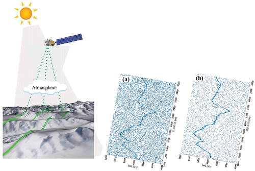
The Advanced Topographic Laser Altimeter System (ATLAS) is the world’s first spaceborne photon-counting laser altimeter for Earth observation, providing detailed parameters in Table 1 (Neumann et al. 2019). ATLAS was launched on the Ice, Cloud, and Land Elevation Satellite-2 (ICESat-2) in September 2018, which has been in orbit for 4 years and has gathered massive amounts of global surface photon data. Due to its extremely high measurement accuracy, it has played a significant role in polar ice cover monitoring (Khan et al. 2022), vegetation height estimation (Juan et al. 2022; A. B. Liu, Cheng, and Chen 2021), lake water level measurement (Feng et al. 2023), land surface control point extraction (Lian et al. 2022), and shallow sea bottom measurement (Caballero and Stumpf 2023; X. C. Zhang et al. 2022) and has achieved many research results. However, affected by factors such as solar radiation, atmospheric scattering light intensity, and dark counting, many noise photons are present in spaceborne single-photon laser data, so research on photon denoising is the basis for the application of these photons in various industries.

Table 1. ATLAS laser basic parameters.

Parameter	Value	Parameter	Value
Single pulse energy	120/30 µJ	Orbit height	~500 km
Divergence angle	35 µrad	Dead time	3.2 ns
Wavelength	532 nm	time-to-digital converter (TDC)	200 ps
Repetition frequency	10 kHz	Emission efficiency	0.40
Pulse full width at half-maximum	1.5 ns	Receiving efficiency	0.41
Receiving telescope diameter	0.792 m	Photon detection efficiency	0.15

At present, there is a wealth of research in the field of denoising spaceborne single-photon laser data, which fall broadly categorized into three types. One type is denoising based on raster images (B. Chen and Pang 2015; Magruder et al. 2012), where the photons are transformed into an image, and image processing techniques are utilized to remove noise. This method necessitates the transformation of the laser photons into raster images, a process that could lead to the loss of valuable information. The second type, machine learning-based denoising (Lu et al. 2021; Meng et al. 2022), involves achieving noise removal in spaceborne single-photon laser data by extracting features from the photons. The method requires only a small number of features and is easy to implement, but it is not yet widely used due to the current lack of labeled data. The third type is denoising based on two-dimensional profile photons, where the spatial density differences between signal and noise photons are exploited to separate noise. Denoising methods based on two-dimensional profile photons commonly include density-based spatial clustering denoising (Tian and Shan 2023; J. Zhang and Kerekes 2015; Zhu et al. 2021) and denoising based on local statistics (Neuenschwander and Pitts 2019; Wang, Pan, and Glennie 2016). Among these methods, one of the most frequently employed denoising methods for single-photon data acquired from ATLAS is density-based spatial clustering. Density-based spatial clustering methods include density-based spatial clustering of applications with noise (DBSCAN) (Ester et al. 1996) and ordering points to identify the clustering structure (OPTICS) (Ankerst et al. 1999). Huang et al. proposed the algorithm of particle swarm optimization DBSCAN (Huang et al. 2019), optimized the two parameters of DBSCAN, and improved the applicability of the DBSCAN method. Zhang and Kerekes proposed an elliptical DBSCAN denoising method (J. Zhang and Kerekes 2015), modifying the circular search neighborhood to an ellipse, which significantly improved the denoising accuracy of photons for flat terrain. To adapt to the photon denoising of complex terrain, researchers proposed the directional adaptive ellipse DBSCAN method (DAE-DBSCAN) (Y. F. Chen et al. 2021; Leng et al. 2022), increasing the rotation angle of the ellipse and making it suitable for denoising photon data of complex terrain, such as mountains and sea beds. Tian and Shan conducted a comprehensive analysis of the differences in the density of ground photons and those above in both horizontal and vertical directions to propose a new density-based denoising method (Tian and Shan 2023). Zhu et al. proposed an improved OPTICS denoising method (Zhu et al. 2021) that changed the circular search neighborhood to an ellipse. This method is not sensitive to the neighborhood radius parameter but relies on the minimum number of points in the neighborhood.

The above density-based denoising methods have achieved significant advancements, but they usually modify the search strategy to improve the denoising accuracy. This improved search strategy demonstrates effective noise reduction on different terrains and features under the same noise density conditions. Therefore, these studies only account for the spatial distribution differences of single-photon lasers while neglecting the temporal distribution variations. As shown in Figure 1, solar radiation is the main source of noise in satellite photon counting laser data, and the noise density changes dynamically with the laser observation time, resulting in an uneven noise distribution in the photon cloud. For example, during noon observations (Figure 1a), the noise density is notably higher compared to evening observations (Figure 1b). However, the denoising accuracy of noise removal algorithms based on density-based spatial clustering is mainly determined by their key input parameters (neighborhood radius $\mathit{Eps}$ and the minimum number of points $\mathit{MinPts}$ in the neighborhood) under different noise density conditions. All the aforementioned studies used a constant neighborhood radius and minimum number of points for denoising and have not yet undertaken research on the adaptive optimization of key denoising input parameters. Density clustering algorithms with constant parameters cannot adapt to the denoising of photons under different time conditions, resulting in poor denoising accuracy.

Figure 1. Illustrations of the laser photons under different time conditions. (a) Distribution of signal and noise photons observed at noon; (b) Distribution of signal and noise photons observed in the evening.

For the above issue, a novel spaceborne photon-counting laser altimeter denoising method based on parameter-adaptive density clustering is proposed in this study. Taking DAE-DBSCAN as an example, the spaceborne single-photon laser noise and signal photon data were simulated against the background photon counting rate ($\mathit{bckgrd}\_\mathit{rate}$) of 1–30 MHz. Then, the denoising accuracy ($\mathit{F}$ value) under all conditions was calculated by setting different neighborhood radii and minimum numbers of points. Then, a mathematical prediction model was established with $\mathit{bckgrd}\_\mathit{rate}$ as the independent variable and $\mathit{Eps}$ and $\mathit{MinPts}$ as dependent variables. Finally, the parameter prediction model was used as the input, and the input parameters were adjusted in real time according to the background photon counting rate of actual photon data. The denoising accuracy of the simulated photons for typical terrain and the photons measured by ATLAS was then verified.

2. Materials and methods

2.1. Study area and dataset

2.1.1. Study area

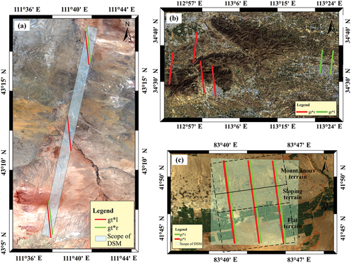
The study area in this study was divided into three regions of China: Erenhot in Inner Mongolia, Songshan in Henan, and Kuqa in Xinjiang. The study area in Erenhot had flat, sandy terrain with an area of approximately 30 km², as shown in Figure 2(a). In Songshan, there were common surface types, such as buildings, farmland, forests, and pastures, as shown in Figure 2(b). Kuqa includes three types of landforms: flat land, slopes, and mountains. The area of the study area is approximately 260 km², as shown in Figure 2(c). The Erenhot experimental area was used for quantifying the key parameters of DAE-DBSCAN denoising and verifying the denoising accuracy of simulated photon data. The Songshan study area was used for ATLAS real-observation photon denoising accuracy verification. The Xinjiang study area was used for the verification of the denoising accuracy of three typical terrains: flat land, slopes, and mountains.

Figure 2. Distribution of the study areas in this paper and the ATLAS data. (a) Inner Mongolia Erenhot experimental area; (b) Henan Songshan experimental area; (c) Xinjiang Kuqa experimental area.

2.1.2. ATLAS and DSM datasets

In this study, ATLAS was taken as the research object, and the experimental data were divided into four categories according to the research aim: (1) data used to quantify the key parameters of DAE-DBSCAN denoising; (2) data used to verify the denoising accuracies of different methods; (3) data used to verify the denoising accuracy of the ATLAS real observation photons; and (4) data used to verify the denoising accuracy for typical terrain. Their details are shown in Table 2. The ATLAS photon data manually labeled by Zhang et al. (https://github.com/Weikiii/WHU-PCL) were adopted as the data of the Songshan study area, where the noise was labeled 1 and the signal was labeled 0 (G. Zhang et al. 2022). The labeled signal photons were used as real signals to verify the accuracy of the denoising as specified in this study. The remaining experimental data used the laser footprint coordinates provided by ATL03 to simulate the echo photon data and to label the signal photons and noise photons of the ground-based simulation.

Table 2. ATLAS data in this study.

Study area	ATLAS file	Beam	Purpose
Erenhot	ATL03_20200403061741_01180702	gt2l	Quantification of key parameters
		gt1l, gt1r, gt3l, gt3r	Verification of denoising accuracy by different methods
Songshan	ATL03_20190725062644_04150406	gt2l, gt3l	ATLAS real observation photon denoising accuracy verification
	ATL03_20190925033040_13600406	gt1r, gt3r
	ATL03_20200502045345_05600702	gt2r, gt3r
Kuqa	ATL03_20210124180132_048510021	gt1l–gt3r	Typical terrain denoising accuracy verification

The development of spaceborne photon counting laser simulation relies on high-precision ground reference terrain data. Therefore, airborne light detection and ranging (LiDAR) was used to obtain high-precision LiDAR point cloud data of the Erenhot and Kuqa study areas, and after postprocessing, DSM data with a resolution of 1.0 m and an elevation accuracy better than 0.1 m were obtained. The obtained DSM adopted the three-dimensional belt projected coordinate system of CGCS2000, and the elevation was the geodetic height of WGS84. The DSM data range is shown by the light blue quadrilaterals in Figure 2(a,c).

2.2. Methods

In this study, we proposed a key parameter quantification and adaptive method based on density clustering denoising. The overall process of the method is shown in Figure 3. First, the photons from a spaceborne single-photon laser were simulated under different background photon count rates. Subsequently, a grid of key parameters ($\mathit{Eps}$ and $\mathit{MinPts}$) is constructed to serve as input parameters for denoising, and the direction-adaptive elliptical DBSCAN denoising method is employed to denoise all the simulated photons. The key denoising parameters are quantified based on the denoising of simulated photons, and a prediction model of the key denoising parameters is established. Finally, simulated photons and ATLAS observed photons are denoised based on the key parameter prediction model, and denoising accuracy validation is performed.

Figure 3. Overall flowchart of this study.

2.2.1. Simulation of spaceborne single-photon laser echo photons

The operational principles of spaceborne photon counting lasers and spaceborne profile lasers are fundamentally identical, with the sole distinction being in the detection mode of the return signal. Therefore, the return signal energy of the spaceborne single-photon laser can be simulated with reference to the spaceborne profile laser (R. Liu and Xie 2021; Yadav 2010). According to the photoelectric conversion model, the energy of the single-photon laser return signal can be converted into the number of photons as follows:

(1) $N_r=\frac{E_r}{\mathit{hc}/\mathit{\lambda }}{\eta }_q$(1)

where $N_r$ refers to the number of photons returned by the spaceborne single-photon laser; $E_r$ stands for the signal energy returned by the spaceborne single-photon laser; $\mathit{h}$ is Planck’s constant; $\mathit{c}$ is the speed of light; $\mathit{\lambda }$ is the wavelength; and ${\eta }_q$ represents the photon detection efficiency.

The photons arriving at the single-photon laser detector will be identified as photon events with a certain probability. The Monte Carlo method was used to simulate photon events. The specific steps were as follows.

1. The returned photons were sorted by their arrival time at the detector and sliced according to the time-to-digital converter, and the number of photons arriving at the single-photon detector in each time segment was counted to obtain the photon set $\mathit{NT}=\left\{\mathit{N}{T}_1,\mathit{N}{T}_1,\dots ,\mathit{N}{T}_n\right\}$.

2. According to the theory of statistical optics (Goodman 2015), the number of photons triggered on the detector roughly follows the Poisson distribution. Assuming that $N_{\tau }$ photons arrive at the detector within the same time $\mathit{\tau }$, the probability that $\mathit{k}$ photons are responded to by the detector is formula (2).

   (2) $\mathit{P}(\mathit{k},\mathit{\tau })=\frac{{\left(N_{\tau }\right)}^{\mathit{k}}exp\left(-N_{\tau }\right)}{\mathit{k}!}$(2)

where $\mathit{P}(\mathit{k},\mathit{\tau })$ is the probability of detecting $\mathit{k}$ photons within time $\mathit{\tau }$; $N_{\tau }$ is the number of photons arriving at the single-photon detector within time $\mathit{\tau }$.

Then, the probability of one or more photons being detected can be deduced as formula (3).

(3) $\mathit{P}(\mathit{k}\ge 1,\mathit{\tau })=1-exp\left(-N_{\tau }\right)$(3)

where $\mathit{P}(\mathit{k}\ge 1,\mathit{\tau })$ is the probability of detecting one or more photons within time $\mathit{\tau }$.

Thus, the detection probability of the photon set $\mathit{NT}$ is calculated as $\mathit{PT}=\left\{\mathit{P}{T}_1,\mathit{P}{T}_1,\dots ,\mathit{P}{T}_n\right\}$.

1. Based on the Monte Carlo simulation method, $\mathit{n}$ groups of probability set $\mathit{UT}=\left\{\mathit{U}{T}_1,\mathit{U}{T}_1,\dots ,\mathit{U}{T}_n\right\}$ that obeyed the uniform distribution $\mathit{U}\left(0,1\right)$ were generated, which were used as the detector response probability threshold. Then, comparing $\mathit{PT}$ and $\mathit{UT}$, if $\mathit{P}{T}_i>\mathit{U}{T}_i$, a photon event was generated; otherwise, no photon event was generated.

2. The generated photon events were sorted by time, and photon events in the dead time were eliminated to obtain the photon events of the single-laser footprint simulation. Moving the laser footprint to the next one, the simulated photons with all laser footprints were generated by repeating steps (1)-(3).

2.2.2. DAE-DBSCAN denoising principle

Ellipse DBSCAN changes the DBSACN search neighborhood from a circle to an ellipse. Therefore, the key parameters input by the ellipse DBSCAN denoising method also change from 2 to 3. That is, the radius of the circular neighborhood $\mathit{r}\_\mathit{circle}$ has changed to $\mathit{Eps}\_\mathit{a}$ and $\mathit{Eps}\_\mathit{b}$ of the elliptical major and minor semiaxis neighborhoods, respectively, and the minimum number of points inside the ellipse is still $\mathit{MinPts}$. Assuming that any two photons in the photon set are $\mathit{i}(d_i,h_i)$ and $\mathit{j}(d_j,h_j)$, respectively, their elliptical distance $\mathit{dist}(\mathit{i},\mathit{j})$ can be calculated with formula (4).

(4) $\mathit{dist}(\mathit{i},\mathit{j})=\mathit{sqrt}\left({\left(\frac{d_i-d_j}{\mathit{Eps}\_\mathit{a}}\right)}^2+{\left(\frac{h_i-h_j}{\mathit{Eps}\_\mathit{b}}\right)}^2\right)$(4)

where $\mathit{dist}(\mathit{i},\mathit{j})$ is the elliptical distance between photon $\mathit{j}$ and photon $\mathit{i}$; $\mathit{Eps}\_\mathit{a}$ and $\mathit{Eps}\_\mathit{b}$ represent the semimajor axis and semiminor axis of the ellipse, respectively; $d_i$ and $h_i$ represent the along-track distance and elevation of the $\mathit{i}$-th photon, respectively; $d_j$ and $h_j$ represent the along-track distance and elevation of the $\mathit{j}$-th photon, respectively.

The directional adaptive ellipse DBSCAN exhibits improved performance compared to ellipse DBSCAN by adding the ellipse rotation angle. If the ellipse rotation angle was $\mathit{\theta }$, according to formula (4), the elliptical distance of a rotating ellipse is derived as shown in formula (5). Then, formula (6) is used to judge whether photon $\mathit{j}$ is within the neighborhood ellipse of photon $\mathit{i}$. Finally, the number of photons within the neighboring ellipse of photon $\mathit{i}$ is determined. When it is less than the minimum number of points $\mathit{MinPts}$, photon $\mathit{i}$ is considered noise; otherwise, it is a signal photon. For the detailed implementation of the algorithm, refer to (Ester et al. 1996).

(5) $\mathit{dist}(\mathit{i},\mathit{j},\mathit{\theta })=\mathit{sqrt}\left({\left(\frac{\left(d_i-d_j\right)cos\left(-\mathit{\theta }\right)+\left(h_i-h_j\right)sin\left(\mathit{\theta }\right)}{\mathit{Eps}\_\mathit{a}}\right)}^2\text{break}+{\left(\frac{\left(h_i-h_j\right)cos\left(\mathit{\theta }\right)-\left(d_i-d_j\right)sin\left(\mathit{\theta }\right)}{\mathit{Eps}\_\mathit{b}}\right)}^2\right)$(5)

(6) $\left\{\begin{array}{c}\mathit{dist}(\mathit{i},\mathit{j})<1,\mathrm{Photon}\mathit{\hspace{0.17em}}\mathit{j}\mathrm{is}\mathrm{inside}\mathrm{the}\mathrm{ellipse};\\ \mathit{dist}(\mathit{i},\mathit{j})=1,\mathrm{Photon}\mathit{\hspace{0.17em}}\mathit{j}\mathrm{is}\mathrm{on}\mathrm{the}\mathrm{ellipse};\\ \mathit{dist}(\mathit{i},\mathit{j})>1,\mathrm{Photon}\mathit{\hspace{0.17em}}\mathit{j}\mathrm{is}\mathrm{outside}\mathrm{the}\mathrm{ellipse};\end{array}\right.$(6)

where $\mathit{\theta }$ is the ellipse rotation angle and $\mathit{dist}(\mathit{i},\mathit{j},\mathit{\theta })$ is the elliptical distance between photons $\mathit{j}$ and $\mathit{i}$ within the ellipse at a rotation angle of $\mathit{\theta }$.

Nevertheless, the essence of DAE-DBSCAN lies in the adaptive determination of the elliptical rotation angle based on the original photons. This study employs a pyramid layering method to rapidly determine an exact elliptical rotation angle, as illustrated in Figure 4. The method is primarily conducted in three layers, with the specific steps as follows.

Figure 4. Schematic diagram illustrating the search for the optimal rotation angle of an ellipse using pyramid layering. (a), (b), and (c) are experiments on the first, second, and third layers, respectively. The black dotted line indicates the position of the ellipse rotation angle; the red dotted line indicates the position of the ellipse’s optimal rotation angle; and the blue solid line is the rotation angle range of the experiment on the next layer.

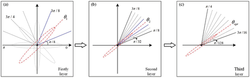
Step 1: The first layer of experiments

As shown in Figure 4(a), for any photon, we first construct the initial search range for the elliptical rotation angle as [0, $\mathit{\pi }$] and divide the search intervals for the rotation angle into one-eighth of the rotation angle search range, which is $\mathit{\pi }/8$ (Leng et al. 2022). This process generates eight potential search ellipses with different orientations, and the number of photons within each potential search ellipse is calculated. The ellipse with the highest number of photons is selected as the optimal ellipse for the current layer, and its rotation angle is denoted as ${\theta }_1$.

Step 2: The second layer of experiments

With the optimal elliptical rotation angle ${\theta }_1$ determined in the first layer as the center, we redefine the search range for the elliptical rotation angle as [${\theta }_1-\mathit{\pi }/8$, ${\theta }_1+\mathit{\pi }/8$], which corresponds to the angles before and after the optimal ellipse rotation angle ${\theta }_1$. The search interval for the rotation angle is set to 1/8 ($\mathit{\pi }/32$) of the rotation angle search range, as shown in Figure 4(b). Then, a new set of eight potential search ellipses with different orientations is reconstructed, and the number of photons within these new potential search ellipses is calculated. The ellipse containing the highest number of photons is considered to have the second-layer determined optimal elliptical rotation angle, denoted as ${\theta }_2$.

Step 3: The last layer of experiments

The rotation angle search process for this layer is completely repeated as in the second layer experiment. In this layer, the search range for the ellipse rotation angle is set to [${\theta }_2-\mathit{\pi }/32$, ${\theta }_2+\mathit{\pi }/32$], with an interval of $\mathit{\pi }/128$, as shown in Figure 4(c). Similarly, eight search ellipses are reconstructed, the ellipse with the highest number of photons inside is determined as the optimal ellipse obtained from the pyramid-layered search, and the optimal ellipse rotation angle is denoted as ${\theta }_{\mathit{opt}}$. Finally, the current experimental photon is moved to the next photon, and steps 1–3 are repeated sequentially to determine the ellipse rotation angles for all the photons.

2.2.3. Quantitative evaluation index of photon denoising accuracy

The accuracy of photon denoising is usually evaluated with the harmonic mean $\mathit{F}$ (J. Zhang and Kerekes 2015) of recall rate $\mathit{R}$ and accuracy $\mathit{P}$ as an index (formulas (7)-(9)). The recall rate $\mathit{R}$ represents the ratio of the number of correctly extracted signal photons to the total number of real signal photons. The accuracy $\mathit{P}$ is the ratio of the number of correctly extracted signal photons to the total number of all signal photons extracted. A harmonic mean $\mathit{F}$ of 1 indicates a high denoising accuracy.

(7) $\mathit{R}=\frac{\mathit{TP}}{\mathit{TP}+\mathit{FN}}$(7)

(8) $\mathit{P}=\frac{\mathit{TP}}{\mathit{TP}+\mathit{FP}}$(8)

(9) $\mathit{F}=\frac{2\mathit{R}\times \mathit{P}}{\mathit{R}+\mathit{P}}$(9)

where $\mathit{TP}$ is the number of signal photons that are correctly identified; $\mathit{FN}$ is the number of signal photons that are not correctly identified among the actual signal photons; and $\mathit{FP}$ is the number of actual noise photons that are misclassified as signal photons.

2.2.4. Construction of key parameter prediction models and photon denoising

According to Figure 3, the process of constructing a prediction model for the key parameters of DAE-DBSCAN and photon denoising is divided into the following four steps.

(1) Photons simulation with different background photon counting rates.

After querying the background photon counting rate recorded by ATLAS, the spaceborne laser background photon counting rate did not exceed 30 MHz under actual conditions. According to the simulation method specified in Section 2.2.1, the simulation of spaceborne single-photon data at a background photon counting rate of 1–30 MHz was completed, where noise was labeled 0 and signals were labeled 1.

(2) Simulation photon denoising based on DAE-DBSCAN.

Section 2.2.2 shows that there are three denoising parameters in DAE-DBSCAN. To improve the feasibility of the experiment, we defined the semimajor axis of the ellipse as twice its semiminor axis (J. Zhang and Kerekes 2015): $\mathit{Eps}\_\mathit{a}=2\mathit{Eps}$, $\mathit{Eps}\_\mathit{b}=\mathit{Eps}$. The key parameters for denoising were thus reduced to two ($\mathit{Eps}$ and $\mathit{MinPts}$). Considering that the along-track interval of the ATLAS footprint was approximately 0.7 m, the dead time is 3.2 ns (approximately 0.96 m). Therefore, the range of the ellipse search neighborhood radius $\mathit{Eps}$ was set to [0.6 m, 5 m], and the minimum number of points $\mathit{MinPts}$ ranged from [2, 15]. Then, the neighborhood radius and minimum number of points grids were generated at intervals of 0.1 m and 1, respectively. For the simulated photon data of 1–30 MHz, DAE-DBSCAN denoising was carried out with all neighborhood radii and the minimum number of points grid data as input parameters. Additionally, the denoising accuracy ($\mathit{F}$ value) corresponding to each key parameter grid is also simultaneously calculated.

(3) Construction of the key parameter prediction model for DAE-DBSCAN denoising.

At any background photon counting rate, the maximum $\mathit{F}$ value was found, and its corresponding neighborhood radius $\mathit{Eps}$ and minimum number of points $\mathit{MinPts}$ were set as the optimal values of key parameters under the current background photon counting rate. The optimal values of the key denoising parameters under all background photon counting rates were repeatedly calculated, and a set $\mathit{NS}$ of background photon counting rates and key parameters was constructed, as shown in formula (10):

(10) $\mathit{NS}=\left\{\begin{array}{c}\left(\mathit{bckgr}{d}_1,\mathit{F}\mathrm{\_}{max}_1,\mathit{Eps}\_\mathit{op}{t}_1,\mathit{MinPts}\_\mathit{op}{t}_1\right),\\ \left(\mathit{bckgr}{d}_2,\mathit{F}\mathrm{\_}{max}_2,\mathit{Eps}\_\mathit{op}{t}_2,\mathit{MinPts}\_\mathit{op}{t}_2\right),\dots \\ \left(\mathit{bckgr}{d}_{30},\mathit{F}\mathrm{\_}{max}_{30},\mathit{Eps}\_\mathit{op}{t}_{30},\mathit{MinPts}\_\mathit{op}{t}_{30}\right)\end{array}\right\}$(10)

where $\mathit{bckgr}{d}_i$ is the $\mathit{i}$-th background photon counting rate; $\mathit{F}\mathrm{\_}\underset{i}{max}$ is the highest denoising accuracy; and $\mathit{Eps}\_\mathit{op}{t}_i$ and $\mathit{MinPts}\_\mathit{op}{t}_i$ are optimal denoising parameters.

Finally, the background photon count rates are used to create separate two-dimensional scatter plots with denoising accuracy, neighborhood radius, and minimum point count. Then, according to the scatter plots, different mathematical statistical models are used to fit the mathematical relationship between each key denoising parameter and background photon count rate, and the fitted mathematical statistical model is used as the key parameter prediction model.

(4) Denoising and verification of photons based on the key parameter prediction model.

If there is a photon set $\mathit{NP}$, $\mathit{NP}$ will be divided into $\mathit{n}$ segments according to the time interval of 0.1 s to obtain a subset $\mathit{NP}=\left\{\mathit{N}{P}_1,\mathit{N}{P}_2,\dots ,\mathit{N}{P}_n\right\}$. Any subset in $\mathit{NP}$ was selected to convert the photon time into the distance value along the track, and the local noise photons were obtained according to the simple local distance statistics method (Zhu et al. 2018). The background photon counting rate (He et al. 2013) in the current subset is calculated. The background photon counting rate is input into the key parameter prediction model to obtain the neighborhood radius and minimum number of points of the current photon set. Then, DAE-DBSCAN was used to complete the current subset photon denoising. All subsets in $\mathit{NP}$ are traversed to achieve denoising of the entire photon set. Finally, the denoising accuracy was verified by using the signal and noise labels in the photon set.

3. Results

3.1. DAE-DBSCAN denoising key parameter quantification

3.1.1. Simulation of echo photons with different background noises

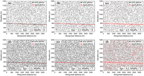
In this study, ATLAS gt2l in the Erenhot study area was taken as the experimental object, and the class 4 photons were obtained as the surface signal photons (Tony, Beata, and Tom 2022) according to the signal photon labels provided by the ATL03 data. Due to multiple signal photons in the same laser pulse, the mean values of latitude, longitude, and elevation of all signal photons in the same pulse were taken as the surface footprint center of the pulse laser. In the experiment, the ATLAS parameters in Table 1 were used as the simulation input parameters, and the DSM elevation in the entire footprint was obtained by using the center position of the laser footprint calculated from the ATL03 data. Finally, the surface echo photon simulation of gt2l was conducted according to the photon simulation method specified in Section 2.2.1. During the simulation, the background photon counting rate was set to 1–30 MHz, and the interval was 1 MHz. A total of 30 sets of photon data were simulated, nine of which are shown in Figure 5.

Figure 5. gt2l simulation results of ATLAS in the Erenhot experimental area. (a)–(i) show the simulated photons under different background photon counting rates: 1 MHz, 3 MHz, 5 MHz, 7 MHz, 10 MHz, 15 MHz, 20 MHz, 25 MHz, and 30 MHz, respectively.

3.1.2. DAE-DBSCAN key parameter quantification

First, the DAE-DBSCAN method was employed to remove noise from 30 sets of simulated photon data, and the denoising parameters, including the neighborhood radius and minimum number of points, were configured in accordance with Step (2) in Section 2.2.4. A total of 630 denoising experiments were conducted for each group of simulated photons. Figure 6 shows the denoising results for three sets of different neighborhood radii and minimum numbers of point parameters under the conditions of a 5 MHz and a 10 MHz background photon counting rate. The results indicate that variations in the key parameters lead to significant differences in the denoising outcomes. The phenomenon of over denoising occurred, as shown in Figure 6c,f. The phenomenon of under denoising also occurred, as shown in Figure 6a,d. In addition, given the same denoising parameters, the denoising results of different background photon counting rate values were also different, with a greater background photon counting rate indicating that more signal photons were wrongly identified. Figure 6b,e are the optimal denoising results at the 5 MHz and 10 MHz background photon counting rates, respectively.

Figure 6. Three groups of denoising results with different parameters at 5 MHz and 10 MHz background photon counting rates. (a)–(c) are the results under the 5 MHz background photon counting rate; (d)–(f) are the results under the 10 MHz background photon counting rate.

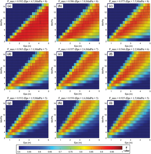
To quantify the accuracy under all denoising parameters, the denoising accuracy ($\mathit{F}$ value) under the current parameter was calculated after each denoising iteration using labeled signal photons. After completing the neighborhood radius and minimum number of points grid traversal, each set of simulated photon data generated a three-dimensional dataset of neighborhood radius, minimum number of points, and $\mathit{F}$ value, and there was a total of 30 sets. Among them, the $\mathit{F}$ value distribution of the nine groups of simulated photons in Figure 5 after denoising is shown in Figure 7. The results demonstrated significant variations in denoising accuracies when different denoising parameters were applied. There was a discernible trend of decreasing denoising accuracy with an increase in background photon counting rate, although the decline in accuracy was not pronounced.

Figure 7. Denoising accuracy with different neighborhood radii $\mathit{Eps}$ and minimum numbers of points $\mathit{MinPts}$. (a)–(i) denoising accuracy at background photon counting rates of 1, 3, 5, 7, 10, 15, 20, 25, and 30 MHz, respectively.

3.1.3. DAE-DBSCAN key parameter prediction model establishment

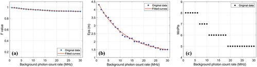
The quantification results of the denoising key parameters of 1–30 MHz are plotted as a scatter plot in Figure 8. The results showed that the background photon counting rate was negatively correlated with the denoising accuracy $\mathit{F}$, neighborhood radius $\mathit{Eps}$, and minimum number of points $\mathit{MinPts}$. Since the background photon counting rate recorded by ATLAS during the noon period is usually less than 30 MHz, these values will not become outliers as the background photon counting rate increases. According to the data trends in Figure 8a,b, the one-dimensional quadratic polynomial and compound exponential function models were used, respectively, to fit the relationship between the background photon counting rate and the values of $\mathit{F}$ and neighborhood radius. The fitted results are shown in formula (11) and formula (12), respectively. Figure 8(c) shows that no strict mathematical model relationship existed between the background photon counting rate and the minimum number of points but rather a piecewise constant relationship. The prediction model of the background photon counting rate and minimum number of points is shown in formula (13).

Figure 8. The relationship between background photon counting rate and denoising parameters. (a) denoising accuracy $\mathit{F}$ value; (b) Ellipse neighborhood $\mathit{Eps}$; (c) minimum number of points $\mathit{MinPts}$ within the neighborhood.

(11) $y_F=0.000087\cdot x_{bc\mathrm{kgrd}\_\mathit{rate}}^2-0.00499\cdot x_{\mathit{bckgrd}\_\mathit{rate}}+0.998219$(11)

(12) $y_{\mathit{Eps}}=3.195\cdot e^{-0.09176\cdot {\mathit{x}}_{\mathit{bckgrd}\_\mathit{rate}}}+1.401\cdot e^{-0.00296\cdot {\mathit{x}}_{\mathit{bckgrd}\_\mathit{rate}}}$(12)

(13) $y_{\mathrm{MinPts}}=\left\{\begin{array}{c}8;\cdots x_{\mathit{bckgrd}\_\mathit{rate}}\le 6.5\cdot \mathrm{MHz}\\ 7;\cdots x_{\mathit{bckgrd}\_\mathit{rate}}>6.5\cdot \mathrm{MHz}\mathrm{and}{x}_{\mathit{bckgrd}\_\mathit{rate}}\le 10.5\cdot \mathrm{MHz}\\ 6;\cdots x_{\mathit{bckgrd}\_\mathit{rate}}>10.5\cdot \mathrm{MHz}\mathrm{and}{x}_{\mathit{bckgrd}\_\mathit{rate}}\le 18.5\cdot \mathrm{MHz}\\ 5;\cdots x_{\mathit{bckgrd}\_\mathit{rate}}>18.5\cdot \mathrm{MHz}\end{array}\right.$(13)

where $x_{\mathit{bckgrd}\_\mathit{rate}}$ is the background photon counting rate; $y_F$ is the $\mathit{F}$ value; $y_{\mathit{Eps}}$ is the ellipse neighborhood $\mathit{Eps}$; and $y_{\mathit{MinPts}\mathit{\hspace{0.17em}}}$ is the minimum number of points $\mathit{MinPts}$ in the neighborhood. Note: The hyperparameters (0.00087, −0.00499, and 0.998219) in formula (11) represent the parameter values of the quadratic equation fitted to the discrete data points in Figure 8(a). Similarly, the hyperparameters (3.195, −0.09176, 1.401, and −0.00296) in formula (12) correspond to the parameter values of the complex exponential function fitted to the discrete data points in Figure 8(b). However, the domain values (6.5 MHz, 10.5 MHz, and 18.5 MHz) in formula (13) are the average background photon count rates before and after the variation of $\mathit{MinPts}$ in Figure 8(c).

3.2. Verification of denoising accuracy based on simulated photons

First, gt1l, gt1r, gt3l, and gt3r of ATLAS in the Erenhot experimental area were used as test objects to conduct photon simulation. The beams of gt1l and gt3l were weak beams, with a laser energy set to 30 µJ during the simulation, while gt1r and gt3r were set to 120 µJ. The background photon counting rate was a random value of 1–5 MHz, 6–10 MHz, 11–12 MHz, or 1–15 MHz during gt1l-gt3r simulation. The background photon counting rate switched to a random value every 0.1 s. Three groups of DAE-DBSCAN denoising experiments were conducted for the simulated four-beam photon data. In Experiment I, the key parameter model predicted in this study was used as an input parameter, and the neighborhood radius and minimum number of points were adjusted in real time to complete the denoising of the four beams. In Experiments II and III, constant parameters were used for denoising.$\mathit{Eps}$ and $\mathit{MinPts}$ were set to 3.5 m and 8, respectively (the optimal parameters at 5 MHz) in Experiment II, and they were set to 2.6 m and 7 (the optimal parameters at 10 MHz) in Experiment III. Then, the denoising accuracy was verified by using the labeled signal photons, and the calculated $\mathit{F}$ value results are shown in Table 3. Among them, the three experimental results of gt1l and gt3r are shown in Figure 9.

Figure 9. Three experimental results of gt1l and gt3r. (a)–(c) gt1l; (d)–(f) gt3r. (a) and (d) are experiment I; (b) and (e) are experiment II; and (c), (f) are experiment III. Black dots indicate noise photons, green dots indicate real signal photons, and red dots indicate denoised signal photons.

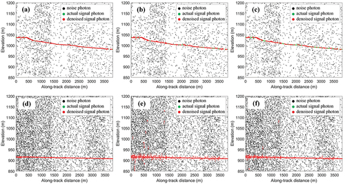
Table 3. DAE-DBSCAN denoising accuracy of the three groups of experiments.

Beam	Background photon counting rate	$\mathit{F}$ value
		Experiment I	Experiment II	Experiment III
gt1l	1–5 MHz	0.975	0.914	0.842
gt1r	6–10 MHz	0.993	0.936	0.950
gt3l	10–15 MHz	0.970	0.821	0.867
gt3r	1–15 MHz	0.992	0.930	0.952

In Figure 9, the denoising results of (a) and (d) are significantly better than those of (b) and (e) or (c) and (f), indicating that the denoising effect of DAE-DBSCAN using the adaptive parameters in this study was significantly better than that of using constant parameters. The results of Table 3 also confirm this conclusion. According to the results of Experiment I to Experiment III in Table 3, the denoising accuracy of gt1r was better than that of gt1l, and the denoising accuracy of gt3r was better than that of gt3l. That is, the denoising accuracy of the strong beam was higher. Regardless of how the background photon counting rate changed, the accuracy of DAE-DBSCAN after denoising using the adaptive parameters in this paper was higher than 0.97. Compared with the constant parameters of Experiments II and III, the denoising accuracy of Experiment I was higher and more stable. In summary, these findings show that the method proposed in this paper is effective and feasible.

4. Discussion

4.1. Denoising analysis of adaptive and constant parameters

For the six beams of ATLAS in the Songshan area, as shown in Figure 2(b), three groups of experiments were conducted, each group of experiments using DAE-DBSCAN for denoising, but their input parameters were different. In Experiment I (adaptive parameters), the key parameter prediction model was used as the input, and the neighborhood radius and minimum number of points were adjusted in real time. In Experiment II (constant parameters), the optimal neighborhood radius and minimum number of points at 15 MHz were used as the input parameters (2.2 m and 6, respectively), and in Experiment III (constant parameters), the optimal neighborhood radius and minimum number of points at 30 MHz were used as the input parameters (1.5 m and 5, respectively). The signal photons manually labeled by G. Zhang et al. (2022) were used as the actual signal photons, and $\mathit{F}$ values of the three groups of experiments were calculated (Table 4). The denoising results of experiments I-III of 20,190,725-gt3l are shown in Figure 10.

Figure 10. 20190725-gt3l three groups of experimental denoising results and enlarged map of mountainous terrain. (a)–(c) are experiments I–III, respectively; (a1)–(c1) are the denoising results of mountainous terrain. Black dots indicate noise photons, green dots indicate real signal photons, and red dots indicate denoised signal photons.

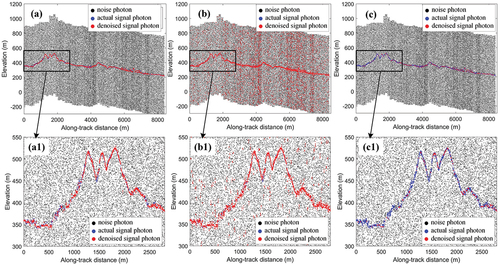
Table 4. ATLAS photon denoising accuracy (F value) in the Songshan experimental area.

Beam	Experiment I	Experiment II	Experiment III
20190725-gt2l	0.954	0.744	0.847
20190725-gt3l	0.961	0.832	0.836
20190925-gt1r	0.957	0.672	0.729
20190925-gt3r	0.966	0.742	0.836
20200502-gt2r	0.978	0.771	0.877
20200502-gt3r	0.953	0.833	0.830

The results in Figure 10 show that over denoising occurred in Experiment II, and many noise photons were identified as signal photons; in Experiment III, under denoising occurred, and many signal photons were not correctly identified, especially in complex mountainous areas. The denoising effect of Experiment I was obviously much better than that of Experiment II and III, and it showed good performance even in complex mountainous areas, as shown in Figure 10a1). According to the $\mathit{F}$ value after denoising of all beams in the experimental area in Table 4, Experiment I has a very high denoising accuracy for the photon data of different ATLAS beams, and the $\mathit{F}$ value was higher than 0.95. However, the denoising accuracy of Experiment II and Experiment III was only approximately 0.8, which again shows that the denoising accuracy of Experiment I was much better than that of Experiments II and III.

In summary, the DAE-DBSCAN adaptive parameters significantly improve the denoising accuracy over constant parameters, and the proposed method shows a satisfactory performance on the real photons of spaceborne lasers with complex terrain.

4.2. Comparative analysis of different denoising methods

To further analyze the reliability of the proposed denoising algorithm (our algorithm), this study compares the proposed method with NASA’s official denoising algorithm (ATL03 and ATL08). NASA has released multiple data products for the ATLAS mission, among which ATL03 and ATL08 products provide signal and noise labels for photons. ATL03 data differentiate photons into noise, low, medium, and high-confidence signal photons using the Poisson statistics method (Neumann et al. 2022). ATL08 employs the differential, regressive, and Gaussian adaptive nearest neighbor (DRAGANN) algorithm for photon denoising (Neuenschwander and Pitts 2019), which categorizes photons into noise, land, canopy, and canopy top signals. Considering the diverse terrains and land cover types in the chosen Songshan experimental area, such as plains, mountains, forests, and urban areas, this section focuses on the six ATLAS beams in the Songshan experimental area (as shown in Figure 2b). The denoising results of our method are compared with ATL03 and ATL08 results, as illustrated in Figure 11. Finally, using manually labeled signal photons as true signal photons, the precision ($\mathit{F}$ value) of ATL03 signal photons with medium and high confidence, as well as AL08 signal photons, was calculated.

Figure 11. Comparison of signal photon labeling results among ATL03 and ATL08 products, along with our own results in the Songshan experimental area. (a) 20190725-gt2l; (b) 20190725-gt3l; (c) 20190925-gt1r; (d) 20190925-gt3r; (e) 20200502-gt2r; (f) 20200502-gt3r.

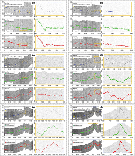
Figure 11 shows the denoising results of the six laser beams in the Songshan experimental area using the ATL03 algorithm, ATL08 algorithm, and our algorithm. It is easy to observe that the denoising accuracy of the ATL03 algorithm is the lowest. The photons extracted with medium to high confidence by this algorithm fail to reflect the real signal photons, resulting in a significant phenomenon of signal loss. However, it must be acknowledged that the denoising accuracy of the ATL08 algorithm is exceptionally high. The signal photons extracted by ATL08 algorithm accurately reflect the shapes of the real surface and features. From the left figure of each laser beam in Figure 11, it is challenging to distinguish the difference in denoising accuracy between our algorithm and the ATL08 algorithm. The partial figure of experimental data in Figure 11 reveals that our algorithm excels in handling details. In complex mountainous terrains, our algorithm exhibits fewer lost signal photons compared to the ATL08 algorithm, as shown in Figure 11(c-f). Additionally, in relatively flat terrains, our algorithm accurately identifies surface signal photons with fewer instances of misidentifying photons above the surface, as seen in Figure 11a,b. This also explains why the $\mathit{F}$ value of our algorithm in Figure 11 is higher than that of the ATL08 algorithm, indicating a higher precision in our algorithm. The comprehensive analysis above thoroughly demonstrates the reliability and high precision of the denoising algorithm proposed in this study.

4.3. Denoising accuracy analysis of typical terrain

To verify the denoising accuracy of the proposed method in different terrains, the echo photons of six beams of ATLAS in the Kuqa study area of Central Xinjiang (Figure 2c) were simulated, and the signal photon and noise photon were labeled. During the simulation, gt*l (where * represents any beam among beams 1 to 3) was a weak beam with a laser energy set to 30 µJ, while gt*r was a strong beam with a laser energy set to 120 µJ. The background photon counting rate for gt1l-gt3r is recorded in the second column of Table 5. For the simulated photon data of each beam, the key parameter prediction model was used as the input, and DAE-DBSCAN denoising was conducted for flat, sloped, and mountainous terrains, and the results are depicted in Figure 12. Here, flat, sloped, and mountainous terrains are defined based on the slope and topographic features. Specifically, terrain with a slope of less than 1 degree is considered flat terrain, terrain with a slope greater than 1 degree and smooth contour is classified as sloped terrain, and terrain with a slope greater than 1 degree and significant undulation is categorized as mountainous terrain. After each denoising iteration, the denoising accuracy ($\mathit{F}$ value) was calculated using the labeled signal photons, and the results are presented in Table 5.

Figure 12. ATLAS simulation photon denoising results of typical terrain. (a)–(f) gt1l, gt2l, gt3l, gt1r, gt2r, and gt3r, respectively. In each subplot, black dots indicate the noise photons, green dots represent the real signal photons, while red, blue, and magenta dots correspond to the signal photons associated with flat land, slopes, and mountainous terrain, respectively.

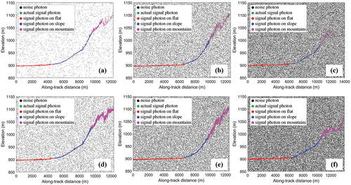
Table 5. Denoising accuracy on typical terrain.

Beam	Background photon counting rate (MHz)	$\mathit{F}$ value
		Flat land	Slope	Mountains
gt1l	1	0.982	0.945	0.921
gt1r	5	0.994	0.979	0.964
gt2l	10	0.977	0.902	0.881
gt2r	15	0.983	0.960	0.914
gt3l	20	0.965	0.898	0.860
gt3r	25	0.976	0.926	0.907

Figure 12 shows that the adaptive parameters model proposed in this study can accurately extract signal photons of strong and weak beams with different background photon counting rates. The strong beam extracted a greater number of signal photons (Figure 12(d–f), whereas the weak beams, particularly in mountainous terrain, extracted fewer signal photons, resulting in some missing data (Figure 12(a–c)). Table 5 clearly indicates that the denoising accuracy of the method proposed in this study is remarkably high on flat surfaces, with $\mathit{F}$values above 0.96. The denoising accuracy in slope terrain is more than 0.9. However, the denoising accuracy in mountainous terrain is relatively poor but still exceeds 0.85. The strong beam denoising accuracy of mountainous terrain is more than 0.9. Therefore, this phenomenon has a certain relationship with the strength of the beam, and gt*r is more accurate than gt*l after denoising, regardless of the terrain. As the background photon counting rate increases, the distance between noise photons decreases, so the distance difference between it and the signal photons of weak beams decreases, resulting in a lower denoising accuracy. The denoising accuracy of the method proposed in this study decreases with the increase in terrain complexity, that is, the denoising accuracy of flat terrain is higher than that of slope terrain and that of mountainous terrain, but they still have high denoising accuracy. In addition, when the background photon counting rate is high, the denoising of the photons with weak pulse energy will also become less accurate.

5. Conclusion

In this study, a novel denoising method for spaceborne photon-counting laser altimeter point clouds based on adaptive parameter density clustering is proposed. Based on the simulated photons, a mathematical prediction model of the background photon counting rate and key parameters of DAE-DBSCAN denoising was established, the optimal denoising parameters were obtained by inputting the background photon counting rate of the actual photons, and the parameters were adjusted in real time. By denoising the simulated photon data with large noise changes, the proposed method denoises with higher accuracy than that when using constant parameters, with $\mathit{F}$ >0.97. We used the same method to verify the denoising accuracy of ATLAS real observation photons. The results show that the method proposed in this study has higher denoising accuracy than models using constant parameters, with $\mathit{F}$ >0.95. In addition, the proposed method is compared with ATL03 and ATL08 denoising algorithm, and the results show that the denoising accuracy of the proposed method is basically the same as the accuracy of the ATL08 algorithm, and both are better than ATL03. Finally, the denoising accuracy of the proposed method on flat land, slope, and mountainous terrain was explored. The results show that the denoising accuracy decreases slightly on more complex terrain, but the accuracy is still high. For example, the denoising accuracy $\mathit{F}$ value of strong-beam laser photons at complex mountainous terrain with a high background photon counting rate can still be higher than 0.9. However, the denoising accuracy of weak-beam laser photons in complex mountains with a high background photon counting rate decreases to 0.86.

The proposed method shows good denoising performance under complex high background photon counting rate and terrain conditions. This method provides a solution to the problem that the parameters of photon denoising based on density clustering are difficult to quantify. However, the proposed method still presents certain limitations in scenarios where the distinction in noise-to-signal photon density is extremely small, attributed to high noise levels and weak signals, particularly evident in photon data extracted from low-energy pulse acquisition in intricate surface landscapes such as mountains and forests. Furthermore, future work should focus on improving the denoising accuracy of photons with weak pulses in complex scenes with a high background photon counting rate. Additionally, further investigation is warranted to determine the precise ratio between the major and minor axes of the search neighborhood ellipse in elliptical DBSCAN.

Disclosure statement

No potential conflict of interest was reported by the author(s).

Data availability statement

The ATLAS data are available from NASA EarthData Search (https://search.earthdata.nasa.gov/search?q=ATLAS).

Additional information

Funding

This work was supported by the Postdoctoral Research Initiation Project of Yunnan Normal University; the Postdoctoral Research Project at the Faculty of Geography, Yunnan Normal University [grant number YNNU-FG-201]; the National Natural Science Foundation of China project [grant number 42371391]; and the Special Funds for Creative Research [grant number 2022C61540].

References

- Ankerst, M., M. M. Breunig, H. P. Kriegel, and J. Sander. 1999. “OPTICS: Ordering Points to Identify the Clustering Structure.” ACM SIGMOD Record 28 (2): 49–19. https://doi.org/10.1145/304181.304187.
- Caballero, I., and R. P. Stumpf. 2023. “Confronting Turbidity, the Major Challenge for Satellite-Derived Coastal Bathymetry.” Science of the Total Environment 870:161898. https://doi.org/10.1016/j.scitotenv.2023.161898.
- Chen, Y. F., Y. Le, D. F. Zhang, Y. Wang, Z. G. Qiu, and L. Z. Wang. 2021. “A Photon-Counting LiDar Bathymetric Method Based on Adaptive Variable Ellipse Filtering.” Remote Sensing of Environment 256:112326. https://doi.org/10.1016/j.rse.2021.112326.
- Chen, B., and Y. Pang. 2015. “A Denoising Approach for Detection of Canopy and Ground from ICESat-2‘s Airborne Simulator Data in Maryland, USA.” AOPC 2015: Advances in Laser Technology and Applications SPIE 9671:383–387. https://doi.org/10.1117/12.2202777.
- Ester, M., H. P. Kriegel, J. Sander, and X. W. Xu. 1996. “A Density-Based Algorithm for Discovering Clusters in Large Spatial Databases with Noise.” Proceedings of the Second International Conference on Knowledge Discovery and Data Mining 96 (34): 226–231. https://dl.acm.org/doi/10.5555/3001460.3001507.
- Feng, Y., L. K. Yang, P. F. Zhan, S. X. Luo, T. Chen, K. Liu, and C. Q. Song. 2023. “Synthesis of the ICESat/ICESat-2 and CryoSat-2 Observations to Reconstruct Time Series of Lake Level.” International Journal of Digital Earth 16 (1): 183–209. https://doi.org/10.1080/17538947.2023.2166134.
- Goodman, J. W. 2015. Statistical Optics. Blackwell: Wiley.
- He, W. J., B. Y. Sima, Y. F. Chen, H. D. Dai, Q. Chen, and G. H. Gu. 2013. “A Correction Method for Range Walk Error in Photon Counting 3D Imaging LIDAR.” Optics Communications 308:211–217. https://doi.org/10.1016/j.optcom.2013.05.040.
- Huang, J. P., Y. Xing, H. You, L. Qin, J. Tian, and J. Ma. 2019. “Particle Swarm Optimization-Based Noise Filtering Algorithm for Photon Cloud Data in Forest Area.” Remote Sensing 11 (8): 980. https://doi.org/10.3390/rs11080980.
- Juan, G. H., L. N. Lana, P. Adri, G. F. Eduardo, B. Brigite, M. Lonesome, N. Amy, C. P. Sorin, and G. Sergio. 2022. “Aboveground Biomass Mapping by Integrating ICESat-2, SENTINEL-1, SENTINEL-2, ALOS2/PALSAR2, and Topographic Information in Mediterranean Forests.” GIScience & Remote Sensing 59 (1): 1509–1533. https://doi.org/10.1080/15481603.2022.2115599.
- Khan, S. A., Y. Choi, M. Morlighem, E. Rignot, V. Helm, A. Humbert, J. Mouginot, R. Millan, K. H. Kjær, and A. A. Bjørk. 2022. “Extensive Inland Thinning and Speed-Up of Northeast Greenland Ice Stream.” Nature 611 (7937): 727–732. https://doi.org/10.1038/s41586-022-05301-z.
- Leng, Z. H., J. Zhang, Y. Ma, J. Y. Zhang, and H. T. Zhu. 2022. “A Novel Bathymetry Signal Photon Extraction Algorithm for Photon-Counting LiDar Based on Adaptive Elliptical Neighborhood.” International Journal of Applied Earth Observation and Geoinformation 115:103080. https://doi.org/10.1016/j.jag.2022.103080.
- Lian, W. Q., G. Zhang, H. Cui, Z. W. Chen, S. D. Wei, C. Y. Zhu, and Z. G. Xie. 2022. “Extraction of High-Accuracy Control Points Using ICESat-2 ATL03 in Urban Areas.” International Journal of Applied Earth Observation and Geoinformation 115:103116. https://doi.org/10.1016/j.jag.2022.103116.
- Liu, A. B., X. Cheng, and Z. Chen. 2021. “Performance Evaluation of GEDI and ICESat-2 Laser Altimeter Data for Terrain and Canopy Height Retrievals.” Remote Sensing of Environment 264:112571. https://doi.org/10.1016/j.rse.2021.112571.
- Liu, R., and J. F. Xie. 2021. “Calibration of the Laser Pointing Bias of the GaoFen-7 Satellite Based on Simulation Waveform Matching.” Optics Express 29 (14): 21844–21858. https://doi.org/10.1364/OE.423679.
- Lu, D., D. Li, X. Zhu, S. Nie, G. Zhou, X. Zhang, and C. Yang. 2021. “ICESat-2 Photon Point Cloud Denoising Classification Based on Convolutional Neural Network.” Journal of Geo-Information Science 23 (11): 2086–2095. https://doi.org/10.12082/dqxxkx.2021.210103.
- Magruder, L. A., M. E. Wharton, K. D. Stout, and A. L. Neuenschwander. 2012. “Noise Filtering Techniques For Photon-counting Ladar Data.” Laser Radar Technology and Applications XVII, SPIE (8397): 237–245. https://doi.org/10.1117/12.919139.
- Meng, W., J. Li, Q. Tang, W. Xu, and Z. Dong. 2022. “ICESat-2 Laser Data Denoising Algorithm Based on a Back Propagation Neural Network.” Applied Optics 61 (28): 8395–8404. https://doi.org/10.1364/AO.469584.
- Neuenschwander, A., and K. Pitts. 2019. “The ATL08 Land and Vegetation Product for the ICESat-2 Mission.” Remote Sensing of Environment 221:247–259. https://doi.org/10.1016/j.rse.2018.11.005.
- Neumann, T. A., A. Brenner, D. Hancock, J. Robbins, A. Gibbons, J. Lee, K. Harbeck, J. Saba, S. Luthcke, and T. Rebold. 2022. “Ice, Cloud, and Land Elevation Satellite (ICESat-2) Project Algorithm Theoretical Basis Document (ATBD) for Global Geolocated Photons ATL03, Version 6.” ICESat-2 Project. https://doi.org/10.5067/GA5KCLJT7LOT.
- Neumann, T. A., A. J. Martino, T. Markus, S. Bae, M. R. Bock, A. C. Brenner, K. M. Brunt, et al. 2019. “The Ice, Cloud, and Land Elevation Satellite-2 Mission: A Global Geolocated Photon Product Derived from the Advanced Topographic Laser Altimeter System.” Remote Sensing of Environment 233:111325. https://doi.org/10.1016/j.rse.2019.111325.
- Tian, X., and J. Shan. 2023. “Detection of Signal and Ground Photons from ICESat-2 ATL03 Data.” IEEE Transactions on Geoscience and Remote Sensing 61:1–14. https://doi.org/10.1109/TGRS.2022.3232053.
- Tony, S., C. Beata, and N. Tom. 2022. “Assessment of ICESat-2’s Horizontal Accuracy Using Precisely Surveyed Terrains in McMurdo Dry Valleys, Antarctica.” IEEE Transactions on Geoscience and Remote Sensing 60:1–11. https://doi.org/10.1109/TGRS.2022.3147722.
- Wang, Z., Z. Pan, and C. Glennie. 2016. “A Novel Noise Filtering Model for Photon-Counting Laser Altimeter Data.” IEEE Geoscience and Remote Sensing Letters 13 (7): 947–951. https://doi.org/10.1109/LGRS.2016.2555308.
- Yadav, G. K. 2010. “Simulation of ICESat/GLAS Full- Waveform over Highly Rugged Terrain. The International Institute.” Master’s thesis., Universit y of Twente Enschede.
- Zhang, J., and J. Kerekes. 2015. “An Adaptive Density-Based Model for Extracting Surface Returns from Photon-Counting Laser Altimeter Data.” IEEE Geoscience and Remote Sensing Letters 12 (4): 726–730. https://doi.org/10.1109/LGRS.2014.2360367.
- Zhang, G., W. Lian, S. Li, H. Cui, M. Jing, and Z. Chen. 2022. “A Self-Adaptive Denoising Algorithm Based on Genetic Algorithm for Photon-Counting Lidar Data.” IEEE Geoscience and Remote Sensing Letters 19:1–5. https://doi.org/10.1109/LGRS.2021.3067609.
- Zhang, X. C., Y. Ma, Z. W. Li, and J. Y. Zhang. 2022. “Satellite Derived Bathymetry Based on ICESat-2 Diffuse Attenuation Signal without Prior Information.” International Journal of Applied Earth Observation and Geoinformation 113:102993. https://doi.org/10.1016/j.jag.2022.102993.
- Zhu, X. X., S. Nie, C. Wang, X. H. Xi, and Z. Y. Hu. 2018. “A Ground Elevation and Vegetation Height Retrieval Algorithm Using Micro-Pulse Photon-Counting Lidar Data.” Remote Sensing 10 (12): 1962. https://doi.org/10.3390/rs10121962.
- Zhu, X. X., S. Nie, C. Wang, X. H. Xi, J. Wang, D. Li, and H. Zhou. 2021. “A Noise Removal Algorithm Based on OPTICS for Photon-Counting LiDar Data.” IEEE Geoscience and Remote Sensing Letters 18 (8): 1471–1475. https://doi.org/10.1109/LGRS.2020.3003191.