Mapping invasive noxious weed species in the alpine grassland ecosystems using very high spatial resolution UAV hyperspectral imagery and a novel deep learning model

ABSTRACT

The term “invasive noxious weed species” (INWS), which refers to noxious weed plants that invade native alpine grasslands, has increasingly become an ecological and economic threat in the alpine grassland ecosystem of the Qinghai-Tibetan Plateau (QTP). Both the INWS and native grass species are small in physical size and share a habitat. Using remote sensing data to distinguish INWS from native alpine grass species remains a challenge. High spatial resolution hyperspectral imagery provides an alternative for addressing this problem. Here, we explored the use of unmanned aerial vehicle (UAV) hyperspectral imagery and deep learning methods with a small sample size for mapping the INWS in mixed alpine grasslands. To assess the method, UAV hyperspectral data with a very high spatial resolution of 2 cm were collected from the study site, and a novel convolutional neural network (CNN) model called 3D&2D-INWS-CNN was developed to take full advantage of the rich information provided by the imagery. The results indicate that the proposed 3D&2D-INWS-CNN model applied to the collected imagery for mapping INWS and native species with small ground truth training samples is robust and sufficient, with an overall classification accuracy exceeding 95% and a kappa value of 98.67%. The F1 score for each native species and INWS ranged from 92% to 99%. In conclusion, our results highlight the potential of using very high spatial resolution UAV hyperspectral data combined with a state-of-the-art deep learning model for INWS mapping even with small training samples in degraded alpine grassland ecosystems. Studies such as ours can aid the development of invasive species management practices and provide more data for decision-making in controlling the spread of invasive species in similar grassland ecosystems or, more widely, in terrestrial ecosystems.

KEYWORDS:

• Invasive noxious weed species (INWS)
• very-high spatial resolution
• UAV hyperspectral imagery
• convolutional neural networks
• alpine grassland ecosystem
• Qinghai-Tibetan Plateau (QTP)

1. Introduction

Invasive noxious weed species (INWS) are typically toxic plants and forbs that have substantial adverse ecosystem functions and economic effects (Gholizadeh, Friedman, et al. 2022; Kettenring and Reinhardt Adams 2011; Zhou et al. 2005). INWS replace native species (Kumar Rai and Singh 2020), are poisonous to livestock due to their oxalic acid content (Valente et al. 2022), alter grassland structure (Nininahazwe et al. 2023), modify the function of native ecosystems (Davies and Johnson 2011; Xing et al. 2021) and homogenize the local flora and fauna (Pejchar and Mooney 2009). Due to their rapid invasion and expansion, the INWS ultimately establishes a dominant population, which has several negative impacts on grassland ecosystems: lowering grassland diversity, reducing pasture quality, resulting in livestock production reduction, and affecting human well-being and economic activities across various regions (Mäkinen et al. 2015; Pejchar and Mooney 2009; Rocchini et al. 2015). However, the spread and expansion mechanisms and strategies of the INWS are poorly understood, and the impacts of INWS invasion are spatially complex. INWS can have profound and lasting negative economic and environmental effects on grasslands (Kumar Rai and Singh 2020). The targeted management of INWS requires accurate and spatially explicit approaches for monitoring their distribution patterns over large geographical scales, as well as the development of cost-effective and operational methods for assessing the status of INWS (Elith et al. 2006; Gholizadeh, Friedman, et al. 2022; Xing et al. 2021).

The key to mapping the INWS using remote sensing techniques is detecting the unique structural, textural, spectral, and phenological characteristics of the INWS to distinguish it from native species (Bradley 2014; Laba et al. 2008; Lopatin et al. 2017). Leveraging structural and textural differences requires focusing on distinct spatial patterns of invasive and native species within a neighborhood pixel and is generally conducted using high spatial resolution imagery according to the physical size of invasive species and their polymerization pattern (Frazier and Wang 2011; Magdeline et al. 2010; Rominger and Meyer 2019). For instance, Broom snakeweed has been successfully distinguished from surrounding Texas grasslands using 1.3 m resolution imagery (Yang and Everitt 2010), whereas small plant species such as Rumex require <1 cm resolution unmanned aerial vehicle (UAV) imagery to successfully classify it among the surrounding grasslands in the Netherlands (Valente et al. 2022).

Spectral differentiation requires examining the unique spectral signature that reflects the biochemical characteristics of invasive species that differ from those of native species and is commonly applied to hyperspectral imagery (Lawrence, Wood, and Sheley 2006; Rajee, Padalia, and Kushwaha 2014; Zhang et al. 2022). For example, the invasive noxious Eurasian weed Lepidium latifolium (perennial pepperweed) was detected from cooccurring species using 128-band HyMap imagery based on its unique spectral qualities (Andrew and Ustin 2008). Similarly, two invasive species, Psidium guajava and Hovenia dulcis, were also successfully distinguished from native species based on their sensitive response to Car/Chl, relative water content, and Chla/Chlb at the leaf level (Mallmann et al. 2023). Using phenological distinctness, the INWS and coexisting native species are distinguished based on seasonal or annual phenology, including differences in the timing of greening and senescence, flowering, maximum growth, and fruit and seed production (Andrew and Ustin 2008; Bradley et al. 2018). Leveraging phenological distinctness requires repeated observations to obtain an adequate temporal dataset containing phenological information (Dai et al. 2020). For example, two invasive annual grasses (Cheatgrass and Medusahead) were mapped to the species level based on their differences in the timing of greenness, flowering and setting of seeds in the western Great Basin, USA (Weisberg et al. 2021). Similarly, in remote sensing studies, growing phenology was used to map invasive Morella faya and Ligustrum lucidum (Glossy privet) tree species in Hawaiian rainforests and in central Argentina (Ben and Asner 2013; Hoyos et al. 2010).

Generally, the abundance of INWS in plant communities facilitates their remote detection. The target INWS should be the dominant form or homogenous stand within the vegetation community, and it must also be large enough to match the spatial resolution of the remote sensor (Gholizadeh, Friedman, et al. 2022; K. S. He et al. 2015). Therefore, using remote sensing to map the INWS in grassland ecosystems is particularly challenging. Fortunately, high spatial resolution hyperspectral imagery is becoming increasingly accessible and affordable with the help of UAVs (B. F. R. Davies et al. 2023; Kopeć et al. 2023; Weisberg et al. 2021). For instance, invasive Knotweed species (Fallopia japonica; Fallopia X. bohemica) were successfully mapped using high spatial resolution UAV imagery and a multitemporal classification approach (Martin et al. 2018). Dao, Axiotis, and He (2021) mapped five native and invasive grassland species in Ontario, Canada based on high spatial resolution hyperspectral imagery collected using a UAV platform.

Machine learning (ML) approaches provide a range of classification algorithms for interpreting remote sensing imagery and have been successfully applied in invasive species identification remote sensing (Baron and Hill 2020; Gavier-Pizarro et al. 2012; Michez et al. 2016; Papp et al. 2021). For example, several machine learning algorithms have been successfully applied for classifying INWS, including random forests (RF (Breiman 2001); e.g., (Peerbhay et al. 2016)), support vector machines (SVMs (Mountrakis, Im, and Ogole 2011; Vapnik 1979); e.g., (Piiroinen et al. 2018)), and artificial neural networks (ANNs (Mutanga and Skidmore 2004); e.g., (Abeysinghe et al. 2019)). Although these ML approaches exhibited high performance in distinguishing invasive species from native communities, ML methods (especially supervised ML methods) require feature engineering to select appropriate data transformations and hand-crafted potential variables (spectral indices, texture metrics) from the dataset prior to modeling (Dorigo et al. 2012; Shouse, Liang, and Fei 2013). Defining series-appropriate features is challenging and may require not only extensive expert knowledge and heuristic decisions about the biochemical properties of the species but also information regarding how these electromagnetic attributes interact with the sensor (Kattenborn et al. 2021). Deep learning (DL), a branch of ML, can be used to reveal higher-level features and uncover more complex patterns and hierarchical relationships (e.g. nonlinear relationships) in data, synthesize a large quantity of data, and avoid the need for feature engineering processes owing to multilayers (Kattenborn et al. 2021; Lake et al. 2022; LeCun, Bengio, and Hinton 2015). DL has been suggested to generate more robust and accurate models and provide new pathways for vegetation remote sensing analysis (Kattenborn et al. 2021; Yuan et al. 2020). Convolutional neural networks (CNNs) are among the most commonly used DL algorithms in remote sensing-based vegetation classification (Ma et al. 2019; Yuan et al. 2020). Recently, only a small number of studies have applied these methods for invasive species identification (Charles et al. 2021; Hasan et al. 2021; Kattenborn et al. 2020; Rodríguez-Garlito, Paz-Gallardo, and Plaza 2023).

Despite the promising results observed using these DL approaches with remote sensing applications (Hasan et al. 2021), we identified three research gaps that currently limit the wide application of DL methods for mapping INWS with remote sensing in grassland ecosystems. First, due to the great and complicated diversity of grasslands, small size of invasive species, and co-occurrence of invasive and native species, it is challenging to discriminate invasive plants from the native grass community (Lam et al. 2020; Valente et al. 2022; Yanhui et al. 2022). To overcome these difficulties, very high spatial resolution and hyperspectral imagery have been used, resulting in a marked increase in dataset volume, as well as an increase in spatial and spectral autocorrelation. This, indeed, has led to an increase in the accuracy of the algorithms but decreased the speed of the processing procedure (Belgiu and Drăguţ 2016; Javier et al. 2022; Maggiori et al. 2017). Second, an advantage of DL is its use of more complex and deeper-level structures to learn more features; hence, a large amount of labeled training data is required to avoid overfitting. Third, the mainstream DL model itself and the large data volume in very high-resolution and hyperspectral imagery both require high computing resources to achieve the desired performance. However, the number of labeled ground-truth samples/datasets for mapping invasive species using remote sensing data is often quite limited (Javier et al. 2022; Kattenborn et al. 2021). There are multiple data is reasons for this limitation, such as missing remote sensing data, inappropriate spatial/spectral resolution data, insufficient experimental samples and expensive computing power.

The main purpose of this study was to use the powerful capability of CNNs in classification tasks and the advantages of high spatial resolution and hyperspectral imagery to map the INWS in alpine grassland ecosystems using small ground truth samples. To achieve the above objective, we formulated the following research hypotheses:

1. The INWS can be distinguished from native species and other ground objects using very high spatial resolution hyperspectral imagery and the DL method in mixed alpine grassland ecosystems, and

2. DL algorithms with well-designed structures can be used to classify INWS using small samples and achieved an acceptable level of accuracy (accuracy >90%).

To test our proposed research hypotheses, we collected UAV hyperspectral data with very high spatial resolution (2 cm), as well as a suite of ground truth information, from the alpine grassland ecosystem of the Qinghai-Tibetan Plateau (QTP). We designed a reasonable CNN model and applied the well-trained CNN model to identify the INWS using small samples.

2. Materials and methods

2.1. Study area

The study area is in the eastern part of the QTP, Northwest China, at an average elevation over 4500 m, a latitude of 35.21° N, and a longitude of 98.97° E (Figure 1). Alpine grasslands are a typical vegetation cover type and occupy more than 85% of the area in this region (Xing et al. 2021). The dominant native species in this area are Kobresia pygmaea, Kobresia humilis, Kobresia capillifolia, Stipa purpurea, Carex moorcroftii, and Brylkinia caudata, and the cooccurring species in this grassland type are Herbarum variorum, Stipa aliena, Ptilagrostis spp., Poa spp., and Leymus secalinus. The main invasive noxious weed species are Ajania tenuifolia, Oxytropis ochrocephala, Euphorbia fischeriana, Aconitum pendulum, Aster altaicus, Leontopodium leontopodioides, Carex himalaica, and Potentilla chinensis (Figure 2) (An et al. 2018; Guo et al. 2020; Liu, Xu, and Shao 2008b; Station 2012; Wang and Kang 2011; Xing et al. 2021, 2023). Unlike introduced invasive alien species, INWS are native invasive species and currently represent one of the major threats to the alpine grassland ecosystem of the QTP (Liu, Xu, and Shao 2008a; Xing et al. 2021; Zhou et al. 2005). We selected the four most abundant targeted INWS (Carex himalaica, Ajania tenuifolia, Oxytropis ochrocephala,and Leontopodium leontopodioides) and three native species in our survey area (Figure 2). The targeted INWS species both contain toxins and foul smells that feature an unpalatable taste and are therefore inedible or poisonous for native livestock (mostly Yak and Tibet sheep in our study area), always causing losses to local herdsmen. The data acquisition site was selected due to its homogenous vegetation community, ease of access, and sufficient quantities of native and INWS, which appeared to provide a representative ground truth sample in the study area.

Figure 1. Location of the study site. (a) UAV color composite image (RGB bands 52, 25, and 7 composite) taken on 19 August 2019, at the study site. The numbers in the image show the control points, the black boxes in the image are the all-subplot boxes, and the nine red boxes are the selected representative data plots shown in Figure 4. (a1) Global-scale location of the study site. (a2) location of the study site on the local scale on the QTP.

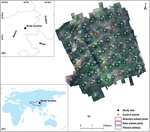
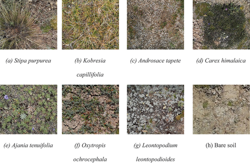
Figure 2. The main native and INW species in our study sites (photographed by the research team using a digital camera in the ground sampling area during field work). The species in pictures (a), (b) and (c) are native species, and those in (c) to (g) are INW species.

2.2. Data acquisition and processing

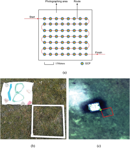
UAV imagery was collected on 19 August 2019, the peak growing season of alpine grassland. The flight route was predesigned and set up in the laboratory (Figure 3(a)) with 85% side overlap and 90% forward overlap in one-way single-flight pass mode. Fifty-six 1 m × 1 m ground reference plots with reference numbers were evenly deployed alongside the flight routes across the collection area, and coordinate information was collected in the bottom right corner of each reference plot. Moreover, the same number of sample plots of the same size were set with the upper left corner in conjunction with the bottom right corner of the reference plot (Figure 3(b,c)). Images were collected from 11:00 am to 1:00 pm (local time) during cloud- and wind-free, sunny weather. The imagery was acquired with 125 spectral bands ranging from 454 to 954 nm using an imaging spectrometer (UHD185 Firefly type, Cubert GmbH, Ulm, Germany) mounted on a six-rotor UAV (Matrice 600 Pro, DJI, Shenzhen, China) platform with six battery modes, flown at an altitude of 100 m and a speed of 8 m/s. Due to the high elevation, each flight time was limited to approximately 13 mins. A standard black and white calibrated reflectance panel was used to eliminate the effect of dark current in hyperspectral cameras and as a reference for calculating reflectance. The final imagery data collected had a 2 cm spatial resolution and 8 nm spectral resolution.

Figure 3. Schematic diagram showing the UAV flight route and ground plot set. (a) UAV flight route design. The red line represents the flight path and heading. The blue circle with a yellow star inside represents the ground control point set. (b) The reference plot and sample plot set used to assist UAV photography and ground truth sample collection on the ground. The white paper with the number represents the reference plot, and the white quadrant in the bottom right corner represents the sample plot. (c) The UAV image of the reference plot and sample plot. The blue polygon represents the reference plot, the red polygon represents the sample plot corresponding to (b), and the green point represents the control point.

The data were collected in two formats: a 1000-pixel by 1000-pixel JPEG format panchromatic image and a 50-pixel by pixel-50 CUE format hyperspectral cube. First, we exported all the data from storage by using Cubert-pilot (Cubert-pilot, Cubert GmbH, Ulm, Germany) and imported the images into PhotoScan (Agisoft PhotoScan Professional, Agisoft LLC, St. Petersburg, Russia), coaligned the images and completed the data mosaic. Afterward, the panchromatic image and hyperspectral cube were fused, and the fifty-six ground control points were used to georeferenced the images into the WGS 1984 UTM Zone 47N projection. Then, the standard reference plot and the shadow were masked from the images to avoid the influence of misclassification. Finally, the resulting digital orthophotographs were obtained.

A field grass species survey was conducted after UAV image acquisition from the fifty-six sample plots (Figure 3(b,c)). Initial vegetation information included plant growth status, grass species composition, bare soil appearance, and the proportion of each class type. Based on our in-situ survey of the dominance of each cover type, the sample plots were classified into two categories: mono-species and mixed growth. The dominant native grass species across the surveyed area were Stipa purpurea, Kobresia capillifolia, and Androsace tapete, and those in the INWS were Ajania tenuifolia, Oxytropis ochrocephala, Leontopodium leontopodioides, and Carex himalaica (Figure 2).

According to the field work results, the ground truth classification samples for each specie classes were selected. Considering that only one grass species appeared in the sample plot and that we could collect pure spectra of this species, we selected nine representative sample sites using the data subset plot (Figure 1(a)) and divided the image into 300 pixels × 300 pixels image patches, which were then used for classification (Figure 4). Within these image patches, we first visually interpreted different cover types. For pixels where the class was more difficult to interpret, we selected the pure spectra of the targeted species and then compared the pixel spectra in a neighborhood, such as the selected species spectrum, to define the proper cover types. Additionally, the reference plot itself and the shadow generated during imaging were eliminated. Because our main goal was to map the INWS with small training samples using CNNs, based on this procedure, we selected only small numbers of pixels (approximately 200 pixels) in total for each class as samples for each image patch. The detailed ground truth sample information is shown in Table 1 (Plot 13 for example). The ground truth color map is shown in Figure 4.

Figure 4. Representative image and ground truths for (a) and (d) plot 13, (b) and (e) plot 15, (c) and (f) plot 22. The composition bands are b52, b25, and b7, and the corresponding wavelengths are 658 nm, 550 nm, and 478 nm, respectively. The black holes in the images are the reference plots and shadows that are masked from the images. We used three of the nine representative images and ground truths as examples, for the remaining images from the nine representative image datasets, please refer to fig. S1.

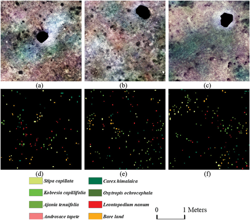
Table 1. Ground truth samples selected for each class.

Classes	Total samples	Trained (70%)	Tested (30%)
Bare soil	232	162	70
Kobresia capillifolia	249	174	75
Stipa purpurea	241	169	72
Androsace tapete	230	161	69
Carex himalaica	241	169	72
Ajania tenuifolia	237	166	71
Oxytropis ochrocephala	172	120	52
Leontopodium leontopodioides	200	140	60

2.3. Principal component analysis (PCA)

Principal component analysis (PCA) is arguably the most popular and widely used mathematical technique for large dataset volume reduction (Abid et al. 2018; Salem and Hussein 2019). The PCA technique aims to transform a dataset with several correlated variables into a smaller set of principal components (PCs), reducing dimensionality while retaining maximal variance and information (e.g. energy) (Guo et al. 2021). Particularly useful for high-dimensional hyperspectral images, PCA identifies and reduces correlations among neighboring spectral bands, analogous to eigenvalue decomposition of the covariance matrix for transformation (Rodarmel and Shan 2002). The new optimum linear combination of the original spectral bands generated after PCA reduction helps to filter noise and uncover hidden structures of the original dataset. Notably, the first few PCs can retain more than 80% of the information present in the original datasets. In this study, PCA was performed on the full spectrum of all nine hyperspectral image cubes in MATLAB (R2023a, The WorkMaths Inc., Mass. USA) to find the most representative PCs of the hyperspectral images we collected.

2.4. CNN building

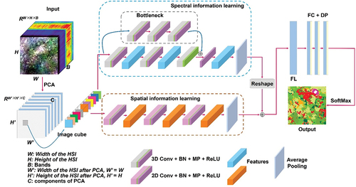
In this study, to make full use of the high spatial resolution and rich spectral information of the collected imagery, we proposed a novel CNN model called the 3D&2D-INWS-CNN model to capture the rich features of the INWS provided by UAV data sources. The overall structure of the CNN model includes image input, data processing and dimension reduction, INWS feature learning and classification, and result outputs. The novel CNN model used a small training sample to identify the INWS with less training data and computational cost. The architecture of our CNN model is shown in Figure 5.

Figure 5. The architecture of our proposed 3D&2D-INWS-CNN model. ‘2D/3D conv + BN + MP + ReLU’ is expressed as a 2D/3D convolution layer, batch normalization (BN) layer, max pooling (MP) layer, and a nonlinear activation function ‘ReLU;’ ‘FL’ is a flattened layer; ‘FC + DP’ is a fully connected layer and dropout; and ‘SoftMax’ is a classifier.

The original hyperspectral image (HSI) data collected in this study can be represented as a three-dimensional (3D) data volume $\mathit{R}$ ($\mathit{R}$ is the original 3D HSI data volume), where the width and height of the HSI data volume are $\mathit{W}$ and$\mathit{H}$, respectively, which are considered two spatial dimensions; $\mathit{B}$ is the number of spectral bands, considered the spectral dimension of the HSI data cube; therefore, the original HSI data cube can be expressed as ${\mathbb{R}}^{\mathit{W}\times \mathit{H}\times \mathit{B}}$. $\mathit{I}$ is the HSI data cube extracted from the original HSI data volume $\mathit{R}$ with wide $\mathit{w}$ and height $\mathit{h}$, and the bands of the data cube $\mathit{I}$ are the same as $\mathit{R}$; therefore, each $I^{\mathit{w}\times \mathit{h}\times \mathit{B}}\in {\mathbb{R}}^{\mathit{W}\times \mathit{H}\times \mathit{B}}$ and $\mathit{I}$ is the HSI data cube used for the INWS identification test. In this study, we have nine different HSI data cubes $\mathit{I}$.

Before implementing our CNN model, a PCA algorithm was applied to reduce the dimensional redundancy of the HSI data cube $\mathit{I}$, and the principal component bands were selected to construct the new image patches that were input into the CNN model (Appice and Malerba 2019). Afterward, the newly constructed input image patch $\mathit{X}$ can be expressed as $X^{w^{\prime }\times h^{\prime }\times \mathit{c}}$, where $X^{w^{\prime }\times h^{\prime }\times \mathit{c}}\in I^{\mathit{w}\times \mathit{h}\times \mathit{B}}$, $w^{\prime }$, and $h^{\prime }$ are the width and height of the image cube $\mathit{X}$, $w^{\prime }=\mathit{w}$ and $h^{\prime }=\mathit{h}$, and $\mathit{c}$ is the number of bands $\mathit{X}$ or principle components. Then, the image patches were input into the 3D conv-learning block to learn spectral features and the 2D conv-learning block to learn spatial information. Next, the learned spectral and spatial features were connected and used for classification.

The 3D&2D-INWS-CNN model consists of two brunch structures, and each brunch consists of convolutional, max pooling, and activation structures that feature spectral learning and spatial learning blocks, respectively. In the spectral learning block, we first defined a skip connection convolution block with three 3D convolution layers with a kernel size of 1 × 1 × 1 and strides of 1 × 1 × 1. The padding was set as “same” in the CNN model building. The input image patches were first convolved by this block. Then, the input data were convolved by a spectral learning block that contained three 3D convolution layers. Each layer had 64 filters with a size of 1 × 1 × 1. In the conv layer, a batch normalization (BN) (Ioffe and Christian 2015) layer and a rectified linear unit (ReLU) (Alex, Sutskever, and Hinton 2012; K. He et al. 2015) activation function were added following each convolution. The skip connection convolution block was added back to the third convolution layer before the ReLU. In the spatial learning block, the input image patches were convolved with three 2D convolution layers. Each conv layer had a kernel size and stride of 3 × 3 × 3, and the padding was also set to “same” in the spatial feature learning block, while the first layer had 128 filters, and the second two layers both had 64 filters. A ReLU activation function was added behind each convolution layer. Then, two max pooling (MP) (Szegedy et al. 2015) layers were added behind the 2D/3D convolution block to reduce the model complexity and computation time. Next, the features learned by the spectral learning block were reshaped to two dimensions and connected with the features learned by the spatial learning block. Finally, the connected features were passed through a flattened layer (FL) (Deep and Zheng 2019), which transformed the features into a feature vector (Jin, Dundar, and Culurciello 2014). Then, three fully connected layers (Basha et al. 2020) with a dropout activation (S.-H. Wang et al. 2020) (FL + DP) and a SoftMax function (LeCun, Bengio, and Hinton 2015) were designed for final classification, and the feature vectors were classified into eight classes in our study (Table 1).

In the CNN classification test, the patch size or so-called window size is an important parameter in a designed CNN architecture. The input patch size affects the number of features extracted by convolution layers in the CNN architecture, and the patch size during the testing period can affect the final classification accuracy (Fang et al. 2019; Kavzoğlu and Özlem Yilmaz 2022), while an appropriate patch size will be beneficial to the classification (Jiang et al. 2021). A previous study demonstrated that the patch size can vary with a moderate spatial resolution (Sharma et al. 2017). Therefore, we tested different patch sizes during the experiment to evaluate how the patch size affects the INWS classification performance. The base parameter settings of our experiment based on the public dataset were as follows: the learning rate was set to 0.001, the batch size was set to 64, the window size was set to a range of 3 × 3, 5 × 5, 7 × 7, 9 × 9, 11 × 11, 13 × 13, 15 × 15, 17 × 17, and 19 × 19, the training epochs were set to 100, and the training/testing ratio was set to 0.7/0.3. The overall accuracy (OA), average accuracy (AA), kappa coefficient (Kappa), user accuracy (UA), producer accuracy (PA), and F1 score (F1) (Maxwell et al. 2021a, 2021b) were used to evaluate the model performance. All the experiments were carried out on Windows 10, Intel i7–8700, NVIDIA Ge Force GTX 1660 (16 GB RAM) with a computing capability of 7.5 and 32 GB of memory. The CNN model was built based on the TensorFlow 2.10.0 framework in the Python 3.9 environment.

3. Results

3.1. Spectral signature of the INWS from UAV data source

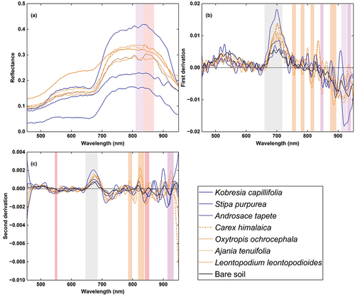
Figure 6 shows the spectral signatures of the three native species (Stipa purpurea, Kobresia capillifolia, and Androsace tapete), four INWS (Ajania tenuifolia, Oxytropis ochrocephala, Leontopodium leontopodioides, and Carex himalaica) and bare soil derived from UAV-based data sources. In general, as shown in Figure 6(a), according to the original spectral signature, the reflectance of all ground features in the data source is low, and the highest albedo is lower than 0.5. Specifically, the native species Androsace tapete had the lowest reflectance in the full spectral range. The native species Kobresia capillifolia showed the highest reflectance in the red edge and near infrared bands (702 nm to 950 nm), and Stipa purpurea also showed an obvious difference in spectral signature reflectance in the red edge and near infrared ranges (the second lowest reflectance from 702 nm to 922 nm). In contrast, for the INWS, in the original spectral signature, the INWS did not show an obvious distinction, and there are only two narrow ranges (810 nm to 834 nm and 834 nm to 870 nm) that can distinguish Ajania tenuifolia and Leontopodium leontopodioides. However, the spectrum transform provides more opportunities for INWS identification. Figure 6(b,c) show that for the derivative spectral signature, the reflectance albedo was between −0.02 and 0.02, and the reflectance of the native species was more distinctive than that of the INWS. For example, Kobresia capillifolia exhibited the highest reflectance in the red edge bands (680 nm to 710 nm) but the lowest in the near-infrared bands (910 nm to 950 nm), and Stipa purpurea exhibited very distinctive spectral features at 900 nm to 920 nm. The reflectance of the INWS was mostly distributed in the near-infrared bands; for example, Ajania tenuifolia exhibited distinctive features at 750 nm to 762 nm, 778 nm to 790 nm, 810 nm to 822 nm, and 874 nm to 894 nm. Carex himalaica and Oxytropis ochrocephala were mostly at wavelength ranging from 842 nm to 852 nm, 930 nm to 942 nm and from 910 nm to 928 nm, respectively. Figure 6 shows that there were wider spectral bands for native species discrimination in the UAV hyperspectral data source, while the spectral band differences between the INWSs were narrower. The native species also exhibited more distinctive spectral characteristics, while the spectra for INWS were more mixed. This indicates that native species are easier to distinguish from UAV hyperspectral data sources; however, there are still opportunities for INWS identification because of the characteristic band of the INWS.

Figure 6. Spectral characteristics of the INWS from UAV hyperspectral sources at our study site. (a) Original reflectance. (b) First derivative reflectance. (c) Second derivative reflectance. The reflectance signatures are blue for native species and orange for INWS.

3.2. Principal component analysis (PCA) band selection

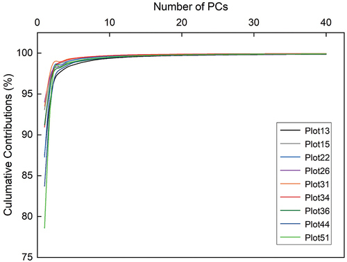
PCA was employed to reduce the band redundancy of the original hyperspectral image cubes, and the cumulative contribution rates of the spectra of the nine hyperspectral cubes are shown in Figure 7. For the nine hyperspectral image cubes, the first principal component (PC1) explained more than 75% of the variance in the hyperspectral image data; five hyperspectral image cubes explained more than 90% of the variance in the hyperspectral data; three image cubes explained 80% to 90% of the variance; and only one image cube explained 78.6% of the variance. The first ten principal components (PC1-PC10) for all nine hyperspectral image cubes explained more than 99% of the variance. The combined contribution of PC2−PC10 varied between 5.44% and 20.92%. None of the principal components alone contain sufficient band information that can explain the original hyperspectral data. In this study, we take the property of the INWS into consideration; only if the cumulative contribution rate reached or exceeded 99.9% was the number of PCs in each hyperspectral image cube selected as the input variables of the DL model. For the original spectra of the nine hyperspectral image cubes, seven of them were selected; the first thirty PCs could explain 99.9% of the total variance, while the other two image cubes need the first forty PCs to reach 99.9% of the total variance of the original hyperspectral image data. Therefore, to unify the standards and facilitate comparison of the experimental results, forty PCs were selected for each hyperspectral image cube that corresponded to 99.9% of the data and were input into the DL model.

Figure 7. The relationship between the number of PCs and the cumulative contributions of nine hyperspectral image cubes.

3.3. INWS classification results

Our 3D&2D-INWS-CNN model was utilized for INWS classification using very high spatial resolution (2 cm) hyperspectral images with small ground truth samples after well-trained. The INWS classification accuracy is reported in Table 2. The results in Table 2 show that overall, the OA, AA, and Kappa were 98.92%, 97.02%, and 98.67%, respectively. Except for the Ajania tapete class, both the UA and PA for the other species and cover types were greater than 90%. For the native species, the classification of Kobresia capillifolia had the highest accuracy, with 98.91% UA, 99.23% PA, and 99.07% F1, while that of Androsace tapete had the lowest PA and F1, which were 87.84% and 92.93%, respectively. This may be because the plant body of Androsace tapete is too small (Figure 2) and easily covered by other INWS and native species; thus, the spectral reflectance is weak and easily mixed with the bare soil that is difficult to capture by the classification model. In contrast, all the INWS classes had promising classification accuracies. For UA, the UA of both Oxytropis ochrocephala and Leontopodium leontopodioides exceeded 98%, which are 98.95% and 98.72%, respectively. The PAs of Carex himalaica and Ajania tenuifolia were also greater than 98%, with values of 98.58% and 98.01%, respectively. The F1 score of Ajania tenuifolia, Oxytropis ochrocephala and Carex himalaica were greater than 96%, with values of 96.65%, 96.58%, and 96.52%, respectively. Additionally, Oxytropis ochrocephala achieved the most accurate combination among the INWS, with 98.95% UA, 93.49% PA, and 96.58% F1 score, even with a narrow spectral range. Furthermore, the other cover types, such as bare soil, also led to a classification accuracy of over 95%. Although there were only narrow feature spectra for some species, acceptable classification accuracy was still achieved for these classes. However, spatial resolution is easier to explain, demonstrating that spatial resolution also plays an important role in INWS identification even when using hyperspectral imagery. In summary, the results indicate that our 3D&2D-INWS-CNN model using high spatial resolution hyperspectral imagery can achieve competitive classification accuracy for INWS classification, even with small ground truth samples.

Table 2. 3D&2D-INWS-CNN model INWS classification accuracy.

	K. C	S. P	A. Te	C. H	L. L	A. Ta	O. O	Bs
UA	98.91	94.78	98.66	94.54	98.72	95.33	98.95	96.57
PA	99.23	93.26	87.84	98.58	92.37	98.01	93.49	98.50
F1	99.07	94.01	92.93	96.52	95.44	96.65	96.58	97.46
OA	98. 92
AA	97.02
K*100	98.67

K. C: Kobresia capillifolia, S. P: Stipa purpurea, A. Te: Androsace tapete, C. H: Carex himalaica, L. L: Leontopodium leontopodioides, A. Ta: Ajania tenuifolia, O. O: Oxytropis ochrocephala, Bs: Bare soil.

We further assessed the impacts of patch size on INWS classification performance. As we can see from Table 3, for the INWS classification accuracy, the highest OA was obtained with a size of 11 × 11, which was 98.92%, and the highest AA appeared with a patch size of 15 × 15, which was not the same as the patch size of OA, and the highest kappa was obtained with a size of 9 × 9. The lowest OA and kappa values of 96.93% and 96.50%, respectively, appeared with a patch size of 3 × 3. The classification results among different patch sizes (Table 3) slightly indicated that a larger patch size will have a better performance for INWS classification than a small patch size. There were 1.99% differences in OA, 2.19% differences in AA, and 2.32% differences in kappa between the highest and lowest classification accuracies among the different patch sizes. However, all the classification accuracies were greater than 95%, and there was no severe variation among the different patch sizes. Therefore, the classification accuracy for all patch sizes seemed to yield acceptable results for the INWS classification in the coexisting environment. The final classification results of INWS for visual analysis were presented in patch size 3 × 3.

Table 3. INWS classification accuracy based on different patch sizes.

	3 × 3	5 × 5	7 × 7	9 × 9	11 × 11	13 × 13	15 × 15	17 × 17	19 × 19
OA	96.93	98.70	98.42	98.85	98.92	97.11	96.97	97.02	98.56
AA	97.11	98.85	96.82	98.56	97.02	96.93	99.01	98.92	98.42
K*100	96.50	98.43	98.14	98.82	98.67	96.81	96.39	96.51	98.26

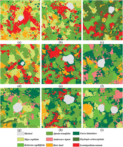
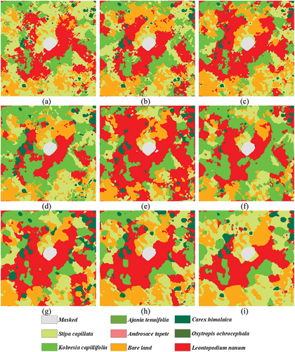
In addition to the quantitative accuracy standard, the visual representation of the classification results was also critical for INWS classification with the CNN model. Figure 8 shows the INWS classification maps of all nine selected subplots as an example. The classification results of the remaining subplots are shown in Fig. S2–Fig. S9. Figure 8 shows that all native species and INWS were well identified in the image with the CNN model. The native species and INWS species had a staggered distribution and composed the vegetation community. Specifically, for native species, Kobresia capillifolia and Stipa purpurea were scattered throughout the vegetation community, while Androsace tapete was sporadic and occupied only a small habitat within the plant community. In contrast, all INWS classes appeared in large patches, covered more space and were distributed in the plant community, especially for Leontopodium leontopodioides and Oxytropis ochrocephala. Based on Figure 8, we concluded that at our study sites, INWS species were dominant in the vegetation community.

Figure 8. Classification map of the INWS. (a): classification result for plot 13. (b): classification result for plot 15. (c): classification for plot 22. (d) Classification result for plot 26. (e) Classification for plot 31. (f) Classification for plot 34. (g) Classification for plot 36. (h) Classification for plot 44. (i) Classification for plot 51.

Figure 9 shows the INWS classification maps with different patch sizes in plot 13 as an example. The classification maps of the remaining patch sizes for the other plots are shown in Fig. S2–Fig. S9. Figure 9 shows that the classification results for the INWS classes in the small patches were scattered, and the edges were rough; however, as the patch size increased, the classification results for each class gathered, and the edges became smoother. These effects were especially obvious for small patches. For example, the small size of Carex himalaica was well scattered in the 3 × 3 and 5 × 5 classification results, but in the larger patch size results, these Carex himalaica were merged into large plaques. Moreover, those classes with large cover were further enlarged, such as the Leontopodium leontopodioides in the INWS and bare soil. Figure 9 indicates that detailed plant information can be well expressed using a small patch size for INWS classification, and there is cross distribution among different INWS classes, which could well present the coexistence status of the INWS species in the natural environment. The classification results with a large patch size provide a smoother classification effect for the INWS class, which indicates that the species have a large distribution pattern and eliminates the possibility of misclassification. Therefore, the classification results with small patch sizes are better for precisely mapping the different INWS species, while the classification results with larger patch sizes could generally be used to present certain INWS classes.

Figure 9. Classification map of the INWS with different patch sizes for plot 13 as an example. (a): 3 × 3. (b): 5 × 5. (c): 7 × 7. (d): 9 × 9. (e): 11 × 11. (f): 13 × 13. (g): 15 × 15. (h): 17 × 17. (i): 19 × 19.

4. Discussion

4.1. UAV high spatial resolution hyperspectral imagery in invasive species mapping

Despite many attempts to monitor and map invasive species through remote sensing approaches in terrestrial ecosystems (Kishore et al. 2022; Piiroinen et al. 2018; Tian et al. 2020; Valente et al. 2022), the detection of invasive species in grassland ecosystems remains a challenging task, and identifying different INWS in mixed alpine grassland ecosystems is even more challenging. We accounted for the spatial and spectral properties of the INWS at our study site: the individual plant body is small, there are differences in the reflectance of different species, and UAV hyperspectral imagery with very high resolution (2 cm) was collected. The novel 3D&2D-INWS-CNN model was proposed to capture the rich features of the INWS from collected UAV data sources that provide high spatial resolution and rich spectral information. Overall, our approach achieved classification accuracies similar to those of previous studies (Kopeć et al. 2023; Nininahazwe et al. 2023).

UAV hyperspectral imagery has long been applied in invasive species identification and mapping due to the advantages of the flexibility of data acquisition and the ability to provide rich spectral bands, making it reliable and acceptable for distinguishing invasive species (Asner et al. 2008; Underwood 2003). Compared to several previous study used UAV hyperspectral imagery to map different invasive species, both obtained an OA above 80% (Gholizadeh, Friedman, et al. 2022; Kishore et al. 2022). In this study, we achieved high-accuracy INWS classification using our collected imagery, which is consistent with the performance of UAV hyperspectral imagery. We studied four INWSs and three native species, whereas other similar studies focused on only one or two species (Gholizadeh, Friedman, et al. 2022; Kishore et al. 2022), demonstrating that the data we collected yielded promising results for mapping INWSs.

Despite the high-performance metrics obtained by the classification model (Table 2), the areal coverage of some species may be overestimated. However, numerous previous studies on remote sensing for invasive species detection have reported problems of under- or overestimation (Gholizadeh, Friedman, et al. 2022; Lass et al. 2002; Lawrence, Wood, and Sheley 2006). We hypothesize that this is mainly due to three closely interconnected issues, namely, species symbiosis, scale mismatch, and spectral mixing, which are common issues in mapping INWS in the TRHR. Furthermore, the issues mentioned above represent the major challenges in invasive species detection using remote sensing approaches; in grassland ecosystems, they are aggravated because the native species and INWS in grassland ecosystems are quite small (Gholizadeh, Dixon, et al. 2022; Gholizadeh, Friedman, et al. 2022). Moreover, these issues also limit the use of satellite-based hyperspectral images because of the coarse spatial resolution of some satellite data sources.

The challenges associated with the small plant size and spatial resolution of remote sensing imagery in mapping the INWS highlighted the importance of spatial resolution in UAV hyperspectral imagery for direct detection of the INWS in grassland ecosystems with small-statured target species (Räsänen and Virtanen 2019). Therefore, we strived to make the best use of the resources at our disposal for collecting UAV high spatial resolution hyperspectral data to overcome the uncertainty in INWS classification. The application of fine spatial resolution hyperspectral imagery to mapping invasive species has become increasingly popular, and the results of our study were in line with those of several similar studies (Elkind et al. 2019; Nininahazwe et al. 2023; Pontius et al. 2017; Schiefer et al. 2020; Tarantino et al. 2019). For example, Glenn et al. (2005) and Lake et al. (2022) both acquired an OA above 90% in detecting a main invasive plant in North America, demonstrating that spatial resolution plays an essential role in mapping invasive species (Glenn et al. 2005; Lake et al. 2022; Schiefer et al. 2020), especially when working with small-statured individual plants (Gholizadeh, Friedman, et al. 2022). The high spatial resolution hyperspectral imagery we collected in this study combines the advantages of both spatial and spectral data that lead to high accuracy in mapping the INWS in alpine grassland ecosystems (Räsänen and Virtanen 2019). Spatial resolution reportedly affects classification accuracy and therefore needs to be further investigated and explored for invasive species detection applications (Roth et al. 2015; Schaaf et al. 2011).

As mentioned above, the high spatial resolution hyperspectral imagery collected by the UAV platform has shown potential for INWS species classification in this study. Therefore, from the aspect of data sources, in the researches that studies that focused on the identification of invasive species, especially invasive species with small plant sizes, high spatial resolution hyperspectral sensors equipped with UAV platforms for the collection of high-quality imagery could be considered a solution for data sources in small-area studies. Furthermore, in studies that cover a larger region, UAV data can also be used as experimental samples and validation data.

4.2. CNN model in invasive species mapping

Compared to the convolutional machine learning approaches reported for detecting invasive species, RF, SVM and extreme gradient boosting (XGBoost) have achieved good results (Lawrence, Wood, and Sheley 2006; Nininahazwe et al. 2023). Compared with ML approaches, CNNs have been successfully used to classify invasive species with better accuracry (Qian et al. 2020). For example, the detection of invasive plant species using CNNs has been demonstrated in different complex landscapes, for which the OA exceeds 95% (Higgisson et al. 2021; Lake et al. 2022). Furthermore, compared to previous research (Hu et al. 2021) conducted in the same area and with the same imagery source as this study but with different ML methods to classify the INWS, the accuracies obtained by our 3D&2D-INWS-CNN model were relatively high, and the OA improved by 5%~6% compared to that of the sparse representation method. Our study demonstrated the ability of CNNs to map invasive species. Although high accuracy was obtained for INWS species classification with the CNN model in this study, there are still several reasons for misclassification, such as the small physical size of the INWS plants, the coexistence of native and INWS species, the mixed spectrum introduced by the coexisted habitat, and the mismatch between the INWS objects and the imagery resolution, either spatially or spectroscopically. In addition, the lack of enough experimental samples also causes misclassification, especially when a DL model is used.

Compared to previous studies, only a few of studies have discussed the impacts of different patch sizes on invasive species mapping with CNNs (Rist et al. 2019), and most of them seem to neglect this point in their reported results (Higgisson et al. 2021; Lake et al. 2022; Qian et al. 2020; Tian et al. 2020). In this study, our results indicated that smaller patch sizes can capture more small species cover, while larger patch sizes can be generalized to present a certain species cover (Figure 9). This finding supported our hypothesis that the different patch sizes used in the CNN model would have an impact on the INWS classification results. However, it cannot be said which patch size is best for INWS classification because both obtained high accuracy in INWS species classification with the proposed CNN model. Therefore, according to the results of this study, identifying and choosing an appropriate patch size for invasive species classification according to a certain purpose is highly recommended for future invasive species classification and mapping applications with CNNs. The reason is that different species present different characteristics (e.g. plant size, height, and form) in imagery, and the features will also be present on different scales, which will affect the final accuracy of the model.

Another concern is that CNNs require a significantly labeled input dataset (Moazzam et al. 2019). However, in the field of remote sensing vegetation or invasive species detection, most of the references thus far have been acquired through ground-based surveys (Fassnacht et al. 2016; James, Bradshaw, and McMahon 2020; Kattenborn et al. 2021), and the quantity of reference data from ground-based surveys is limited by the cost of equipment, personnel, and transportation (Kattenborn et al. 2021). Moreover, the natural environment and accessibility of the study area also greatly limit the amount of reference data collected and the sampling frequency. Several studies have used more than 30,000 labeled images in total to train CNNs to monitor invasive species in practice and achieved high accuracy (Higgisson et al. 2021; Tang, Zhang, and Zhao 2021). Our study area has complex terrain (over 4500 m above sea level) and a harsh environment (a plateau environment). Hence, the effectiveness of CNNs will be restricted by ground-based surveys, especially for complex detection tasks, such as target species or classes with distinctive characteristics that only differ in subtle features (Kattenborn et al. 2021). A common training strategy, data augmentation (Alex, Sutskever, and Hinton 2012; Chatfield et al. 2014), was used in CNN training to compensate for the small reference dataset. Data augmentation artificially inflates the size of the reference dataset by introducing small perturbations (e.g. geometric transformations, color space transformations) to the existing data or by generating simulated data (Shorten and Khoshgoftaar 2019). Several invasive species detection applications with CNNs have used data augmentation to expand training datasets and achieved good performance (Charles et al. 2021; Gibril et al. 2021; Kattenborn et al. 2020; Takaya, Sasaki, and Ise 2022). Although the data augmentation technique offers a solution for training dataset issues, it also introduces another issue: the performance of the CNN depends on the computational resources, and augmenting the reference dataset leads to greater computational costs. Increasing the computing power requires a larger budget because hardware equipment is relatively expensive; this places a financial burden on researchers and may hamper the widespread application of CNNs in invasive species monitoring (Meloni et al. 2019; Yuan et al. 2020). For this reason, more alternative approaches must be proposed to achieve a trade-off of high accuracy performance and few referenced datasets. The authors of a previous study also suggested that deep learning methods are needed to learn from few labeled samples and exploit rich information from related unlabeled data sources (Reichstein et al. 2019). Fortunately, many studies have focused on using small samples in CNN applications (Ahmadi, Mehrshad, and Mohammadali Arghavan 2020; Goodfellow et al. 2020; Hu et al. 2020; Tao et al. 2020; Xue, Zhou, and Du 2022). Compared to previous studies (Zhao et al. 2022), a contrastive self-supervised learning (SSL) algorithm was introduced to address the problems with few labeled samples in hyperspectral classification that used 1% of the samples of the public test dataset and still achieved a high OA (97.69%). However, the use of limited labeled samples in remote sensing invasive species detection fields with CNNs remains rare. In this study, we selected only small ground truth samples (Table 1) and used 70% of them to train our 3D&2D-INWS-CNN model, obtaining a high OA (over 95%) for INWS classification. Therefore, the results of our study suggest that exploring more efficient CNN architectures will help to improve the performance of remote sensing-related invasive species monitoring with small samples in the future, which will also help reduce the sampling collection workload.

4.3. PCA band selection for INWS classification in the DL model

The number of PCs selected for input into the DL model is approximately one-third of the number of bands in the original hyperspectral dataset. A previous study indicated that the more PCs retained with PCA to input into the model, the better the performance of the model (F. Guo et al. 2021). The optimal number of PCs should be determined by the percentage of the cumulative variance of that in the total variance of the original dataset to find the minimum number of PCs that contain the most information of the original datasets. Compared to a previous study (Wang 1999), when the cumulative contribution of the first few principal components was more than 80%, the remaining principal components could be discarded. In this study, most of the hyperspectral image cubes with only PC1 met this requirement. However, a previous study noted that for a model with a PCA band selection process, overfitting and underfitting phenomena also occur (Guo et al. 2021). When many PCs are selected and input into the model, the PCs that represent the noise information are accounted for and introduced into the model, which reduces the model prediction performance, that is overfitting. However, if a small number of PCs were used in the model, it may not fully retain the sufficient information of the original hyperspectral dataset and fully reflect the spectral features of the targeted samples in the original dataset, which would also reduce the model inversion accuracy, that is underfitting. Therefore, in this study, if we follow the 80% rule in a previous study (Liu, Wu, and Huang 2010), the INWS classification may be underestimated, while forty PCs could contain and explain 99.9% of the information in the original hyperspectral datasets; this is not a very large number of PCs compared to the original 125 spectral bands, which is also consistent with the PC selection rule in a previous study (Shahin and Symons 2011).

4.4. Limitations and outlook

The high overall accuracy (over 98%) of the results obtained in the INWS classification using very high spatial resolution UAV hyperspectral imagery with hundreds of narrow spectral bands demonstrated the advantages of the UAV data source in invasive species mapping applications, providing rich spatial and spectral information. The flexibility of data acquisition is another advantage of UAV platforms, especially for inaccessible study areas. There are still some limitations that restrict UAV data source applications in invasive species mapping. First, the amount of UAV imagery collected is limited to a small spatial extent, which restricts large-scale invasive species mapping applications. For example, a previous study using UAV data to classify invasive annual grasses limited the study area to 2.78 ha (Weisberg et al. 2021), a larger scale with a total area of 47 km² (Gholizadeh, Friedman, et al. 2022), while satellite-based sensors can cover a wider spatial extent (Tian et al. 2020). Although the spatial coverage extent of UAVs seems to be a shortcoming when used independently, its application in combination with other data sources will highlight its advantages. For instance, a few studies have used UAV data as an alternative to field sampling to map woody invasive species with Sentinel-1 and Sentinel-2 images (Kattenborn et al. 2019). UAV platform data sources can acquire both high spatial resolution and hyperspectral images but cover only a small scale. Satellite hyperspectral data can cover a large scale, but the spectral resolution and spatial resolution are not sufficient to map small individual invasive plants. Determining how to match both their advantages is still necessary, and this is a problem that we want to explore in future research (Kattenborn et al. 2019).

Second, a previous study demonstrated the contribution of different spectral regions to plant diversity (Wang et al. 2018). For example, studies have reported that the NIR bands achieved the most accurate classification of invasive annual grasses (Weisberg et al. 2021), the shortwave infrared (SWIR) bands included can enhance the ability to map plant (Gholizadeh, Dixon, et al. 2022), and contributions from SWIR regions of the electromagnetic spectrum can uncover significant specific plant function traits, particularly the water content that dominates the reflectance in this region (Carter 1991). Additionally, studies have reported different bands in the visible region (~400 nm-700 nm), red edge region (~700 nm-740 nm), NIR region (~710 nm-1100 nm), and SWIR region (~1100 nm-2450 nm) in the UVA hyperspectra for mapping invasive Lespedeza cuneata (Gholizadeh, Friedman, et al. 2022). We also observed feature bands in the red edge and near infrared bands for distinguishing native species (Kobresia capillifolia: 702 nm to 950 nm, Stipa purpurea: 702 nm to 922 nm) and in the NIR region (810 nm to 834 nm and 834 nm to 870 nm) for distinguishing INWS, such as Ajania tenuifolia and Leontopodium leontopodioides (Figure 6). However, in this study, our hyperspectral data included only a short spectral region that ranged from 450 nm to 950 nm and covered only the visible, red edge and NIR regions, and the characteristics of both the native species and the INWS in the SWIR region remain unknown. To overcome this, we applied the first derivation and second derivation spectrum transforms to explore more information and obtained many spectral features for INWS identification (Figure 6). Therefore, we suggest collecting full spectrum range hyperspectral imagery (if applicable) instead of short-range data under sufficient conditions.

The advantages of the rich information provided by high spatial resolution or hyperspectral imagery for detecting invasive species have been leveraged here and in previous studies (Kattenborn et al. 2019; Wu et al. 2019). However, these advantages are always from the perspective of remote sensing data, and there are also advantages of plants that are beneficial for distinguishing native or invasive species, such as functional traits. Most of the traits used in invasive species detection applications have been plant phenology traits due to their ease of derivation from imagery, and the remaining functional traits of invasive species remain underexplored. However, due to the short growing season in our study area and the mixed habitat of native species and the INWS at our study site, the phenology characteristics of native species and the INWS are quite similar and not sufficient for distinguishing the INWS and native species by means of phenology (Xing et al. 2021). Other functional traits were not explored due to a lack of relevant data, which is a limitation of our study. In future studies, we will focus on more deeply exploring the physiological and biochemical characteristics of native species and INWS and propose additional methods for distinguishing these species. We also suggest considering plant functional traits for future invasive species detection research.

5. Conclusion

In this study, very high spatial resolution (2 cm) UAV hyperspectral imagery of the degraded alpine grassland ecosystem in the TRHR of the QTP was used to classify native and INWS plant species via a novel deep learning-based convolution model. We collected UAV imagery with 125 bands ranging from 450–950 nm with 125 spectral bands. Using the principal component analysis (PCA) dimension reduction method, forty PCs were selected to represent the hyperspectral image dataset. A novel deep learning-based convolutional neural network model called 3D&2D-INWS-CNN was proposed to distinguish invasive noxious weed species (INWS) from native grass species in alpine grassland ecosystems. Based on the results of this study, it could be concluded that the PCA method is efficient for selecting the optimal PCs from multidimensional hyperspectral image data. The 3D&2D-INWS-CNN model combined with very high spatial resolution UAV hyperspectral imagery efficiently distinguished the coexisting INWS from the native species. The CNN model proposed in this study uses a relatively small number of training samples to avoid the high expense of computing resources. The overall classification accuracy of the INWS exceeded 95%, and the classification accuracy of each native species and the INWS exceeded 92%. This study not only provides a novel state-of-the-art method for invasive species mapping but could also aid in the development of invasive species management practices and provide more data for decision making in controlling the spread of invasive species in similar grassland ecosystems or, more widely, in terrestrial ecosystems.

Acknowledgments

The authors show their gratitude to those anonymous reviewers for their insightful comments and suggestions improved the paper. The authors also thank their fellow research colleagues for their help in field data collection.

Disclosure statement

No potential conflict of interest was reported by the author(s).

Data availability statement

All data and source code associated with this paper are available on request.

Supplementary material

Supplemental data for this article can be accessed online at https://doi.org/10.1080/15481603.2024.2327146

Additional information

Funding

This work was supported by the National Key Research and Development Program of China [2023YFC3006505]; National Natural Science Foundation of China [52309017]; National Natural Science Foundation of China [41871326]; Natural Science Foundation of Jiangsu Province [BK20230958]; Key Laboratory of Hydrometeorology of China Meteorological Administration [23SWQXM047]; Natural Sciences and Engineering Research Council of Canada [RGPIN- RGPIN-2022-04471]; China Scholarship Council [202106710115].

References

- Abeysinghe, T., A. Simic Milas, K. Arend, B. Hohman, P. Reil, A. Gregory, and A. Vázquez-Ortega. 2019. “Mapping Invasive Phragmites Australis in the Old Woman Creek Estuary Using UAV Remote Sensing and Machine Learning Classifiers.” Remote Sensing 11 (11): 1380. https://doi.org/10.3390/rs11111380.
- Abid, A., M. J. Zhang, V. K. Bagaria, and J. Zou. 2018. “Exploring Patterns Enriched in a Dataset with Contrastive Principal Component Analysis.” Nature Communications 9 (1): 2134.
- Ahmadi, S. A., N. Mehrshad, and S. Mohammadali Arghavan. 2020. “Spectral-Spatial Classification Method for Hyperspectral Images Using Stacked Sparse Autoencoder Suitable in Limited Labelled Samples Situation.” Geocarto International 37 (7): 2031–25. https://doi.org/10.1080/10106049.2020.1797188.
- Alex, K., I. Sutskever, and G. E. Hinton. 2012. “ImageNet Classification with Deep Convolutional Neural Networks.” Advances in Neural Information Processing Systems 25:1–9. https://doi.org/10.1145/3065386.
- Andrew, M., and S. Ustin. 2008. “The Role of Environmental Context in Mapping Invasive Plants with Hyperspectral Image Data.” Remote Sensing of Environment 112 (12): 4301–4317. https://doi.org/10.1016/j.rse.2008.07.016.
- An, R., C. Lu, H. Wang, D. Jiang, M. Sun, and J. Arthur Quaye Ballard. 2018. “Remote Sensing Identification of Rangeland Degradation Using Hyperion Hyperspectral Image in a Typical Area for Three-River Headwater Region, Qinghai, China (In Chinese.” Geomatics and Information Science of Wuhan University 43 (3): 399–405. https://doi.org/10.13203/j.whugis20150168.
- Appice, A., and D. Malerba. 2019. “Segmentation-Aided Classification of Hyperspectral Data Using Spatial Dependency of Spectral Bands.” Isprs Journal of Photogrammetry & Remote Sensing 147:215–231. https://doi.org/10.1016/j.isprsjprs.2018.11.023.
- Asner, G. P., D. E. Knapp, T. Kennedy-Bowdoin, M. O. Jones, R. E. Martin, J. Boardman, and R. F. Hughes. 2008. “Invasive Species Detection in Hawaiian Rainforests Using Airborne Imaging Spectroscopy and LiDAR.” Remote Sensing of Environment 112 (5): 1942–1955. https://doi.org/10.1016/j.rse.2007.11.016.
- Baron, J., and D. J. Hill. 2020. “Monitoring Grassland Invasion by Spotted Knapweed (Centaurea Maculosa) with RPAS-Acquired Multispectral Imagery.” Remote Sensing of Environment 249. https://doi.org/10.1016/j.rse.2020.112008.
- Basha, S. S., S. Ram Dubey, V. Pulabaigari, and S. Mukherjee. 2020. “Impact of Fully Connected Layers on Performance of Convolutional Neural Networks for Image Classification.” Neurocomputing 378:112–119. https://doi.org/10.1016/j.neucom.2019.10.008.
- Belgiu, M., and L. Drăguţ. 2016. “Random Forest in Remote Sensing: A Review of Applications and Future Directions.” Isprs Journal of Photogrammetry & Remote Sensing 114:24–31. https://doi.org/10.1016/j.isprsjprs.2016.01.011.
- Ben, S., and G. P. Asner. 2013. “Multi-Temporal Hyperspectral Mixture Analysis and Feature Selection for Invasive Species Mapping in Rainforests.” Remote Sensing of Environment 136:14–27. https://doi.org/10.1016/j.rse.2013.04.006.
- Bradley, B. A. 2014. “Remote Detection of Invasive Plants: A Review of Spectral, Textural and Phenological Approaches.” Biological Invasions 16 (7): 1411–1425. https://doi.org/10.1007/s10530-013-0578-9.
- Bradley, B. A., C. A. Curtis, E. J. Fusco, J. T. Abatzoglou, J. K. Balch, S. Dadashi, and M.-N. Tuanmu. 2018. “Cheatgrass (Bromus tectorum) Distribution in the Intermountain Western United States and Its Relationship to Fire Frequency, Seasonality, and Ignitions.” Biological Invasions 20 (6): 1493–1506. https://doi.org/10.1007/s10530-017-1641-8.
- Breiman, L. 2001. “Random Forests.” Machine Learning 45 (1): 5–32. https://doi.org/10.1023/A:1010933404324.
- Carter, G. A. 1991. “Primary and Secondary Effects of Water Content on the Spectral Reflectance of Leaves.” American Journal of Botany 78 (7): 916–924.
- Charles, C. P., P. Henrique Correa Kim, A. G. de Almeida, E. Vieira Do Nascimentok, L. Gianne Souza Da Rocha, and K. Cristiane Teixeira Vivaldini. 2021. “Detection of Invasive Vegetation Through UAV and Deep Learning.” In 2021 Latin American Robotics Symposium (LARS), 2021 Brazilian Symposium on Robotics (SBR), and 2021 Workshop on Robotics in Education (WRE), Natal, Brazil, 114–119.
- Chatfield, K., K. Simonyan, A. Vedaldi, and A. Zisserman. 2014. “Return of the Devil in the Details: Delving Deep into Convolutional Nets.” arXiv preprint arXiv:1405.3531. https://doi.org/10.48550/arXiv.1405.353.
- Dai, J., D. A. Roberts, D. A. Stow, L. An, S. J. Hall, S. T. Yabiku, and P. C. Kyriakidis. 2020. “Mapping Understory Invasive Plant Species with Field and Remotely Sensed Data in Chitwan, Nepal.” Remote Sensing of Environment 250. https://doi.org/10.1016/j.rse.2020.112037.
- Dao, P. D., A. Axiotis, and Y. He. 2021. “Mapping Native and Invasive Grassland Species and Characterizing Topography-Driven Species Dynamics Using High Spatial Resolution Hyperspectral Imagery.” International Journal of Applied Earth Observation and Geoinformation 104. https://doi.org/10.1016/j.jag.2021.102542.
- Davies, B. F. R., P. Gernez, A. Geraud, S. Oiry, P. Rosa, M. Laura Zoffoli, and L. Barillé. 2023. “Multi- and Hyperspectral Classification of Soft-Bottom Intertidal Vegetation Using a Spectral Library for Coastal Biodiversity Remote Sensing.” Remote Sensing of Environment 290. https://doi.org/10.1016/j.rse.2023.113554.
- Davies, K. W., and D. D. Johnson. 2011. “Are We “Missing the Boat” on Preventing the Spread of Invasive Plants in Rangelands?” Invasive Plant Science & Management 4 (1): 166–171. https://doi.org/10.1614/ipsm-d-10-00030.1.
- Deep, S., and X. Zheng. 2019. “Hybrid Model Featuring CNN and LSTM Architecture for Human Activity Recognition on Smartphone Sensor Data.” In Paper presented at the 2019 20th international conference on parallel and distributed computing, applications and technologies (PDCAT), Gold Coast, QLD, Australia.
- Dorigo, W., A. Lucieer, T. Podobnikar, and A. Čarni. 2012. “Mapping Invasive Fallopia Japonica by Combined Spectral, Spatial, and Temporal Analysis of Digital Orthophotos.” International Journal of Applied Earth Observation and Geoinformation 19:185–195. https://doi.org/10.1016/j.jag.2012.05.004.
- Elith, J., C. H. Graham, R. P. Anderson, M. Dudik, S. Ferrier, A. Guisan, R. J. Hijmans, et al. 2006. “Novel Methods Improve Prediction of species’ Distributions from Occurrence Data.” Holarctic Ecology 29 (2): 129–151. https://doi.org/10.1111/j.2006.0906-7590.04596.x.
- Elkind, K., T. T. Sankey, S. M. Munson, C. E. Aslan, and N. Horning. 2019. “Invasive Buffelgrass Detection Using High‐Resolution Satellite and UAV Imagery on Google Earth Engine.” Remote Sensing in Ecology and Conservation 5 (4): 318–331. https://doi.org/10.1002/rse2.116.
- Fang, L., G. Liu, S. Li, P. Ghamisi, and J. Atli Benediktsson. 2019. “Hyperspectral Image Classification with Squeeze Multibias Network.” IEEE Transactions on Geoscience & Remote Sensing 57 (3): 1291–1301. https://doi.org/10.1109/TGRS.2018.2865953.
- Fassnacht, F. E., H. Latifi, K. Stereńczak, A. Modzelewska, M. Lefsky, L. T. Waser, C. Straub, and A. Ghosh. 2016. “Review of Studies on Tree Species Classification from Remotely Sensed Data.” Remote Sensing of Environment 186:64–87. https://doi.org/10.1016/j.rse.2016.08.013.
- Frazier, A. E., and L. Wang. 2011. “Characterizing spatial patterns of invasive species using sub-pixel classifications.” Remote Sensing of Environment 115 (8): 1997–2007. https://doi.org/10.1016/j.rse.2011.04.002.
- Gavier-Pizarro, G. I., T. Kuemmerle, L. E. Hoyos, S. I. Stewart, C. D. Huebner, N. S. Keuler, and V. C. Radeloff. 2012. “Monitoring the Invasion of an Exotic Tree (Ligustrum Lucidum) from 1983 to 2006 with Landsat TM/ETM+ Satellite Data and Support Vector Machines in Córdoba, Argentina.” Remote Sensing of Environment 122:134–145. https://doi.org/10.1016/j.rse.2011.09.023.
- Gholizadeh, H., A. P. Dixon, K. H. Pan, N. A. McMillan, R. G. Hamilton, S. D. Fuhlendorf, J. Cavender-Bares, and J. A. Gamon. 2022. “Using Airborne and DESIS Imaging Spectroscopy to Map Plant Diversity Across the Largest Contiguous Tract of Tallgrass Prairie on Earth.” Remote Sensing of Environment 281. https://doi.org/10.1016/j.rse.2022.113254.
- Gholizadeh, H., M. S. Friedman, N. A. McMillan, W. M. Hammond, K. Hassani, A. V. Sams, M. D. Charles, et al. 2022. “Mapping Invasive Alien Species in Grassland Ecosystems Using Airborne Imaging Spectroscopy and Remotely Observable Vegetation Functional Traits.” Remote Sensing of Environment 271:112887. https://doi.org/10.1016/j.rse.2022.112887.
- Gibril, M. B. A., H. Zulhaidi Mohd Shafri, A. Shanableh, R. Al-Ruzouq, A. Wayayok, and S. Jahari Hashim. 2021. “Deep Convolutional Neural Network for Large-Scale Date Palm Tree Mapping from UAV-Based Images.” Remote Sensing 13:14. https://doi.org/10.3390/rs13142787.
- Glenn, N. F., J. T. Mundt, K. T. Weber, T. S. Prather, L. W. Lass, and J. Pettingill. 2005. “Hyperspectral Data Processing for Repeat Detection of Small Infestations of Leafy Spurge.” Remote Sensing of Environment 95 (3): 399–412. https://doi.org/10.1016/j.rse.2005.01.003.
- Goodfellow, I., J. Pouget-Abadie, M. Mirza, B. Xu, D. Warde-Farley, S. Ozair, A. Courville, and Y. Bengio. 2020. “Generative Adversarial Networks.” Communications of the ACM 63 (11): 139–144. https://doi.org/10.1145/3422622.
- Guo, F., Z. Xu, H. Ma, X. Liu, S. Tang, Z. Yang, L. Zhang, F. Liu, M. Peng, and K. Li. 2021. “Estimating Chromium Concentration in Arable Soil Based on the Optimal Principal Components by Hyperspectral Data.” Ecological Indicators 133:108400. https://doi.org/10.1016/j.ecolind.2021.108400.
- Guo, J., Q. Zhang, M. Song, Y. Shi, B. Zhou, W. Wang, Y. Li, X. Zhao, and H. Zhou. 2020. “Status and Function Improvement Technology of the Grassland Ecosystem in the Upper Yellow River Basin (In Chinese.” Acta Agrestia Sinica 28 (5): 1173–1184. https://doi.org/10.11733/j.issn.1007-0435.2020.05.001.
- Hasan, A. S. M. M., F. Sohel, D. Diepeveen, H. Laga, and G. K. J. Michael. 2021. “A Survey of Deep Learning Techniques for Weed Detection from Images.” Computers and Electronics in Agriculture 184. https://doi.org/10.1016/j.compag.2021.106067.
- He, K. S., B. A. Bradley, A. F. Cord, D. Rocchini, M. Tuanmu, S. Schmidtlein, W. Turner, et al. 2015. “Will Remote Sensing Shape the Next Generation of Species Distribution Models?” Remote Sensing in Ecology and Conservation 1 (1): 4–18. https://doi.org/10.1002/rse2.7.
- He, K., X. Zhang, S. Ren, and J. Sun. 2015. “Delving Deep into Rectifiers: Surpassing Human-Level Performance on Imagenet Classification.” In Paper presented at the Proceedings of the IEEE international conference on computer vision, Santiago, Chile.
- Higgisson, W., A. Cobb, A. Tschierschke, and F. Dyer. 2021. “Estimating the Cover of Phragmites Australis Using Unmanned Aerial Vehicles and Neural Networks in a Semi‐Arid Wetland.” River Research and Applications 37 (9): 1312–1322. https://doi.org/10.1002/rra.3832.
- Hoyos, L. E., G. I. Gavier-Pizarro, T. Kuemmerle, E. H. Bucher, V. C. Radeloff, and P. A. Tecco. 2010. “Invasion of Glossy Privet (Ligustrum Lucidum) and Native Forest Loss in the Sierras Chicas of Córdoba, Argentina.” Biological Invasions 12 (9): 3261–3275. https://doi.org/10.1007/s10530-010-9720-0.
- Hu, Y., R. An, Z. Ai, and W. Du. 2021. “Research on Grass Species Fine Identification Based on UAV Hyperspectral Images in Three-River Source Region.” Remote Sensing Technology and Application 36 (4): 926–935. https://doi.org/10.11873/j.issn.1004‐0323.2021.4.0926.
- Hu, X., Y. Zhong, C. Luo, and X. Wang. 2020. “WHU-Hi: UAV-Borne Hyperspectral with High Spatial Resolution (H2) Benchmark Datasets for Hyperspectral Image Classification.” arXiv preprint arXiv:2012.13920. https://org/10.48550/arXiv.2012.13920.
- Ioffe, S., and S. Christian 2015. “Batch Normalization: Accelerating Deep Network Training by Reducing Internal Covariate Shift.” In Proceedings of the 32nd International Conference on Machine Learning, Lille, France, edited by B. Francis and B. David, 448–456. Proceedings of Machine Learning Research, PMLR.
- James, K., K. Bradshaw, and S. McMahon. 2020. “Detecting Plant Species in the Field with Deep Learning and Drone Technology.” Methods in Ecology and Evolution 11 (11): 1509–1519. https://doi.org/10.1111/2041-210x.13473.
- Javier, M., A. Linstädter, P. Magdon, S. Wöllauer, F. A. Männer, L.-M. Schwarz, G. Ghazaryan, J. Schultz, Z. Malenovský, and O. Dubovyk. 2022. “Predicting Plant Biomass and Species Richness in Temperate Grasslands Across Regions, Time, and Land Management with Remote Sensing and Deep Learning.” Remote Sensing of Environment 282. https://doi.org/10.1016/j.rse.2022.113262.
- Jiang, Y., Y. Li, S. Zou, H. Zhang, and Y. Bai. 2021. “Hyperspectral Image Classification with Spatial Consistence Using Fully Convolutional Spatial Propagation Network.” IEEE Transactions on Geoscience & Remote Sensing 59 (12): 10425–10437. https://doi.org/10.1109/tgrs.2021.3049282.
- Jin, J., A. Dundar, and E. Culurciello. 2014. “Flattened Convolutional Neural Networks for Feedforward Acceleration.” arXiv preprint arXiv:1412.5474. https://doi.org/10.48550/arXiv.1412.5474.
- Kattenborn, T., J. Eichel, S. Wiser, L. Burrows, F. E. Fassnacht, S. Schmidtlein, N. Horning, and N. Clerici. 2020. “Convolutional Neural Networks Accurately Predict Cover Fractions of Plant Species and Communities in Unmanned Aerial Vehicle Imagery.” Remote Sensing in Ecology and Conservation 6 (4): 472–486. https://doi.org/10.1002/rse2.146.
- Kattenborn, T., J. Leitloff, F. Schiefer, and S. Hinz. 2021. “Review on convolutional neural networks (CNN) in vegetation remote sensing.” Isprs Journal of Photogrammetry & Remote Sensing 173:24–49. https://doi.org/10.1016/j.isprsjprs.2020.12.010.
- Kattenborn, T., J. Lopatin, M. Förster, A. Christian Braun, and F. Ewald Fassnacht. 2019. “UAV Data as Alternative to Field Sampling to Map Woody Invasive Species Based on Combined Sentinel-1 and Sentinel-2 Data.” Remote Sensing of Environment 227:61–73. https://doi.org/10.1016/j.rse.2019.03.025.
- Kavzoğlu, T., and E. Özlem Yilmaz. 2022. “Analysis of Patch and Sample Size Effects for 2D-3D CNN Models Using Multiplatform Dataset: Hyperspectral Image Classification of ROSIS and Jilin-1 GP01 Imagery.” Turkish Journal of Electrical Engineering & Computer Sciences 30 (6): 2124–2144. https://doi.org/10.55730/1300-0632.3929.
- Kettenring, K. M., and C. Reinhardt Adams. 2011. “Lessons Learned from Invasive Plant Control Experiments: A Systematic Review and Meta-Analysis.” The Journal of Applied Ecology 48 (4): 970–979. https://doi.org/10.1111/j.1365-2664.2011.01979.x.
- Kishore, B. S. P. C., A. Kumar, P. Saikia, N. Lele, P. Srivastava, S. Pulla, H. Suresh, B. Kumar Bhattarcharya, M. Latif Khan, and R. Sukumar e. 2022. “Mapping of Understorey Invasive Plant Species Clusters of Lantana Camara and Chromolaena Odorata Using Airborne Hyperspectral Remote Snesing.” Advances in Space Research. https://doi.org/10.1016/j.asr.2022.12.026.
- Kopeć, D., A. Zakrzewska, A. Halladin-Dąbrowska, J. Wylazłowska, and Ł. Sławik. 2023. “The Essence of Acquisition Time of Airborne Hyperspectral and On-Ground Reference Data for Classification of Highly Invasive Annual Vine Echinocystis Lobata (Michx.) Torr. & A. Gray.” GIScience & Remote Sensing 60 (1). https://doi.org/10.1080/15481603.2023.2204682.
- Kumar Rai, P., and J. S. Singh. 2020. “Invasive Alien Plant Species: Their Impact on Environment, Ecosystem Services and Human Health.” Ecological Indicators 111:106020. https://doi.org/10.1016/j.ecolind.2019.106020.
- Laba, M., R. Downs, S. Smith, S. Welsh, C. Neider, S. White, M. Richmond, W. Philpot, and P. Baveye. 2008. “Mapping Invasive Wetland Plants in the Hudson River National Estuarine Research Reserve Using Quickbird Satellite Imagery.” Remote Sensing of Environment 112 (1): 286–300. https://doi.org/10.1016/j.rse.2007.05.003.
- Lake, T. A., R. D. Briscoe Runquist, D. A. Moeller, T. Sankey, and Y. Ke. 2022. “Deep Learning Detects Invasive Plant Species Across Complex Landscapes Using Worldview‐2 and Planetscope Satellite Imagery.” Remote Sensing in Ecology and Conservation 8 (6): 875–889. https://doi.org/10.1002/rse2.288.
- Lam, O. H. Y., M. Dogotari, M. Prüm, H. Narendra Vithlani, C. Roers, B. Melville, F. Zimmer, and R. Becker. 2020. “An Open Source Workflow for Weed Mapping in Native Grassland Using Unmanned Aerial Vehicle: Using Rumex Obtusifolius as a Case Study.” European Journal of Remote Sensing 54 (sup1): 71–88. https://doi.org/10.1080/22797254.2020.1793687.
- Lass, L. W., D. C. Thill, B. Shafii, and T. S. Prather. 2002. “Detecting Spotted Knapweed (Centaurea maculosa) with Hyperspectral Remote Sensing Technology.” Weed Technology 16 (2): 426–432. https://doi.org/10.1614/0890-037X(2002)016[0426:DSKCMW]2.0.CO;2.
- Lawrence, R. L., S. D. Wood, and R. L. Sheley. 2006. “Mapping Invasive Plants Using Hyperspectral Imagery and Breiman Cutler Classifications (randomForest.” Remote Sensing of Environment 100 (3): 356–362. https://doi.org/10.1016/j.rse.2005.10.014.
- LeCun, Y., Y. Bengio, and G. Hinton. 2015. “Deep learning.” Nature 521 (7553): 436–444. https://doi.org/10.1038/nature14539.
- Liu, Z.-Y., H.-F. Wu, and J.-F. Huang. 2010. “Application of Neural Networks to Discriminate Fungal Infection Levels in Rice Panicles Using Hyperspectral Reflectance and Principal Components Analysis.” Computers and Electronics in Agriculture 72 (2): 99–106. https://doi.org/10.1016/j.compag.2010.03.003.
- Liu, J., X. Xu, and Q. Shao. 2008a. “Grassland Degradation in the “Three-River Headwaters” Region, Qinghai Province.” Journal of Geographical Sciences 18 (3): 259–273. https://doi.org/10.1007/s11442-008-0259-2.
- Liu, J., X. Xu, and Q. Shao. 2008b. “The Spatial and Temporal Characteristics of Grassland Degradation in the Three-River Headwaters Region in Qinghai Province.” Acta Geographica Scnica 63 (4): 364–376.
- Lopatin, J., F. E. Fassnacht, T. Kattenborn, and S. Schmidtlein. 2017. “Mapping Plant Species in Mixed Grassland Communities Using Close Range Imaging Spectroscopy.” Remote Sensing of Environment 201:12–23. https://doi.org/10.1016/j.rse.2017.08.031.
- Magdeline, L., B. Blair, R. Downs, B. Monger, W. Philpot, S. Smith, P. Sullivan, and P. C. Baveye. 2010. “Use of Textural Measurements to Map Invasive Wetland Plants in the Hudson River National Estuarine Research Reserve with IKONOS Satellite Imagery.” Remote Sensing of Environment 114 (4): 876–886. https://doi.org/10.1016/j.rse.2009.12.002.
- Maggiori, E., Y. Tarabalka, G. Charpiat, and P. Alliez. 2017. “Convolutional Neural Networks for Large-Scale Remote-Sensing Image Classification.” IEEE Transactions on Geoscience & Remote Sensing 55 (2): 645–657. https://doi.org/10.1109/tgrs.2016.2612821.
- Mäkinen, H., J. Kaseva, P. Virkajärvi, and H. Kahiluoto. 2015. “Managing Resilience of Forage Crops to Climate Change Through Response Diversity.” Field Crops Research 183:23–30. https://doi.org/10.1016/j.fcr.2015.07.006.
- Ma, L., Y. Liu, X. Zhang, Y. Ye, G. Yin, and B. Alan Johnson. 2019. “Deep Learning in Remote Sensing Applications: A Meta-Analysis and Review.” Isprs Journal of Photogrammetry & Remote Sensing 152:166–177. https://doi.org/10.1016/j.isprsjprs.2019.04.015.
- Mallmann, C. L., W. Pereira Filho, J. B. B. Dreyer, L. A. Tabaldi, and F. Machado Durgante. 2023. “Leaf-Level Field Spectroscopy to Discriminate Invasive Species (Psidium Guajava L. and Hovenia Dulcis Thunb.) from Native Tree Species in the Southern Brazilian Atlantic Forest.” Remote Sensing 15:3. https://doi.org/10.3390/rs15030791.
- Martin, F.-M., J. Müllerová, L. Borgniet, F. Dommanget, V. Breton, and A. Evette. 2018. “Using Single- and Multi-Date UAV and Satellite Imagery to Accurately Monitor Invasive Knotweed Species.” Remote Sensing 10 (10). https://doi.org/10.3390/rs10101662.
- Maxwell, A. E., T. A. Warner, and L. Andrés Guillén. 2021a. “Accuracy Assessment in Convolutional Neural Network-Based Deep Learning Remote Sensing Studies—Part 1: Literature Review.” Remote Sensing 13 (13): 2450. https://doi.org/10.3390/rs13132450.
- Maxwell, A. E., T. A. Warner, and L. Andrés Guillén. 2021b. “Accuracy Assessment in Convolutional Neural Network-Based Deep Learning Remote Sensing Studies—Part 2: Recommendations and Best Practices.” Remote Sensing 13 (13): 2591. https://doi.org/10.3390/rs13132591.
- Meloni, P., A. Garufi, G. Deriu, M. Carreras, and D. Loi. 2019. “CNN Hardware Acceleration on a Low-Power and Low-Cost ApsoC.” In Paper presented at the 2019 Conference on Design and Architectures for Signal and Image Processing (DASIP), Montreal, QC, Canada.
- Michez, A., H. Piégay, L. Jonathan, H. Claessens, and P. Lejeune. 2016. “Mapping of Riparian Invasive Species with Supervised Classification of Unmanned Aerial System (UAS) Imagery.” International Journal of Applied Earth Observation and Geoinformation 44:88–94. https://doi.org/10.1016/j.jag.2015.06.014.
- Moazzam, S. I., U. Shahbaz Khan, M. Islam Tiwana, J. Iqbal, W. S. Qureshi, and S. Irfan Shah. 2019. “A Review of Application of Deep Learning for Weeds and Crops Classification in Agriculture.” In Paper presented at the 2019 International Conference on Robotics and Automation in Industry (ICRAI), Rawalpindi, Pakistan.
- Mountrakis, G., J. Im, and C. Ogole. 2011. “Support Vector Machines in Remote Sensing: A Review.” Isprs Journal of Photogrammetry & Remote Sensing 66 (3): 247–259. https://doi.org/10.1016/j.isprsjprs.2010.11.001.
- Mutanga, O., and A. K. Skidmore. 2004. “Integrating Imaging Spectroscopy and Neural Networks to Map Grass Quality in the Kruger National Park, South Africa.” Remote Sensing of Environment 90 (1): 104–115. https://doi.org/10.1016/j.rse.2003.12.004.
- Nininahazwe, F., J. Théau, G. Marc Antoine, and M. Varin. 2023. “Mapping Invasive Alien Plant Species with Very High Spatial Resolution and Multi-Date Satellite Imagery Using Object-Based and Machine Learning Techniques: A Comparative Study.” GIScience & Remote Sensing 60 (1). https://doi.org/10.1080/15481603.2023.2190203.
- Papp, L., B. van Leeuwen, P. Szilassi, Z. Tobak, J. Szatmári, M. Árvai, J. Mészáros, and L. Pásztor. 2021. “Monitoring Invasive Plant Species Using Hyperspectral Remote Sensing Data.” Land 10 (29): 1–18. https://doi.org/10.3390/land10010029.
- Peerbhay, K., O. Mutanga, R. Lottering, and R. Ismail. 2016. “Mapping Solanum Mauritianum Plant Invasions Using WorldView-2 Imagery and Unsupervised Random Forests.” Remote Sensing of Environment 182:39–48. https://doi.org/10.1016/j.rse.2016.04.025.
- Pejchar, L., and H. A. Mooney. 2009. “Invasive Species, Ecosystem Services and Human Well-Being.” Trends in Ecology & Evolution 24 (9): 497–504. https://doi.org/10.1016/j.tree.2009.03.016.
- Piiroinen, R., F. Ewald Fassnacht, J. Heiskanen, E. Maeda, B. Mack, and P. Pellikka. 2018. “Invasive Tree Species Detection in the Eastern Arc Mountains Biodiversity Hotspot Using One Class Classification.” Remote Sensing of Environment 218:119–131. https://doi.org/10.1016/j.rse.2018.09.018.
- Pontius, J., R. P. Hanavan, R. A. Hallett, B. D. Cook, and L. A. Corp. 2017. “High Spatial Resolution Spectral Unmixing for Mapping Ash Species Across a Complex Urban Environment.” Remote Sensing of Environment 199:360–369. https://doi.org/10.1016/j.rse.2017.07.027.
- Qian, W. Q., Y. Q. Huang, Q. Liu, W. Fan, Z. Y. Sun, H. Dong, F. H. Wan, and X. Qiao. 2020. “UAV and a Deep Convolutional Neural Network for Monitoring Invasive Alien Plants in the Wild.” Computers and Electronics in Agriculture 174. https://doi.org/10.1016/j.compag.2020.105519.
- Rajee, G., H. Padalia, and S. P. S. Kushwaha. 2014. “Forest Tree Species Discrimination in Western Himalaya Using EO-1 Hyperion.” International Journal of Applied Earth Observation and Geoinformation 28:140–149. https://doi.org/10.1016/j.jag.2013.11.011.
- Räsänen, A., and T. Virtanen. 2019. “Data and Resolution Requirements in Mapping Vegetation in Spatially Heterogeneous Landscapes.” Remote Sensing of Environment 230. https://doi.org/10.1016/j.rse.2019.05.026.
- Reichstein, M., G. Camps-Valls, B. Stevens, M. Jung, J. Denzler, N. Carvalhais, and Prabhat. 2019. “Deep Learning and Process Understanding for Data-Driven Earth System Science.” Nature 566 (7743): 195–204. https://doi.org/10.1038/s41586-019-0912-1.
- Rist, Y., I. Shendryk, F. Diakogiannis, and S. Levick. 2019. “Weed Mapping Using Very High Resolution Satellite Imagery and Fully Convolutional Neural Network.” In IGARSS 2019–2019, Ieee International Geoscience and Remote Sensing Symposium, Yokohama, Japan, 9784–9787.
- Rocchini, D., V. Andreo, M. Förster, C. Ximena Garzon-Lopez, A. Paul Gutierrez, T. W. Gillespie, H. C. Hauffe, et al. 2015. “Potential of Remote Sensing to Predict Species Invasions.” Progress in Physical Geography: Earth and Environment 39 (3): 283–309. https://doi.org/10.1177/0309133315574659.
- Rodarmel, C., and J. Shan. 2002. “Principal Component Analysis for Hyperspectral Image Classification.” Surveying and Land Information Science 62 (2): 115–122.
- Rodríguez-Garlito, E. C., A. Paz-Gallardo, and A. Plaza. 2023. “Mapping Invasive Aquatic Plants in Sentinel-2 Images Using Convolutional Neural Networks Trained with Spectral Indices.” IEEE Journal of Selected Topics in Applied Earth Observations & Remote Sensing 16:2889–2899. https://doi.org/10.1109/jstars.2023.3257142.
- Rominger, K., and S. Meyer. 2019. “Application of UAV-Based Methodology for Census of an Endangered Plant Species in a Fragile Habitat.” Remote Sensing 11:6. https://doi.org/10.3390/rs11060719.
- Roth, K. L., D. A. Roberts, P. E. Dennison, M. Alonzo, S. H. Peterson, and M. Beland. 2015. “Differentiating Plant Species within and Across Diverse Ecosystems with Imaging Spectroscopy.” Remote Sensing of Environment 167:135–151. https://doi.org/10.1016/j.rse.2015.05.007.
- Salem, N., and S. Hussein. 2019. “Data Dimensional Reduction and Principal Components Analysis.” Procedia Computer Science 163:292–299. https://doi.org/10.1016/j.procs.2019.12.111.
- Schaaf, A. N., P. E. Dennison, G. K. Fryer, K. L. Roth, and D. A. Roberts. 2011. “Mapping Plant Functional Types at Multiple Spatial Resolutions Using Imaging Spectrometer Data.” GIScience & Remote Sensing 48 (3): 324–344. https://doi.org/10.2747/1548-1603.48.3.324.
- Schiefer, F., T. Kattenborn, A. Frick, J. Frey, P. Schall, B. Koch, and S. Schmidtlein. 2020. “Mapping Forest Tree Species in High Resolution UAV-Based RGB-Imagery by Means of Convolutional Neural Networks.” Isprs Journal of Photogrammetry & Remote Sensing 170:205–215. https://doi.org/10.1016/j.isprsjprs.2020.10.015.
- Shahin, M. A., and S. J. Symons. 2011. “Detection of Fusarium Damaged Kernels in Canada Western Red Spring Wheat Using Visible/near-Infrared Hyperspectral Imaging and Principal Component Analysis.” Computers and Electronics in Agriculture 75 (1): 107–112. https://doi.org/10.1016/j.compag.2010.10.004.
- Sharma, A., X. Liu, X. Yang, and D. Shi. 2017. “A Patch-Based Convolutional Neural Network for Remote Sensing Image Classification.” Neural Networks: The Official Journal of the International Neural Network Society 95:19–28. https://doi.org/10.1016/j.neunet.2017.07.017.
- Shorten, C., and T. M. Khoshgoftaar. 2019. “A survey on image data augmentation for deep learning.” Journal of Big Data 6 (1): 1–48.
- Shouse, M., L. Liang, and S. Fei. 2013. “Identification of Understory Invasive Exotic Plants with Remote Sensing in Urban Forests.” International Journal of Applied Earth Observation and Geoinformation 21:525–534. https://doi.org/10.1016/j.jag.2012.07.010.
- Station, Q. R. W. 2012. Grassland Resources of Qinghai. Xining: Qinghai People’s Publish Press Co., Ltd.
- Szegedy, C., W. Liu, Y. Q. Jia, P. Sermanet, S. Reed, D. Anguelov, D. Erhan, V. Vanhoucke, and A. Rabinovich. 2015. “Going deeper with onvolutions.” 2015 Ieee Conference on Computer Vision and Pattern Recognition (Cvpr), 1–9. https://doi.org/10.1109/cvpr.2015.7298594.
- Takaya, K., Y. Sasaki, and T. Ise. 2022. “Automatic Detection of Alien Plant Species in Action Camera Images Using the Chopped Picture Method and the Potential of Citizen Science.” Breeding Science 72 (1): 96–106. https://doi.org/10.1270/jsbbs.21062.
- Tang, F., D. Zhang, and X. Zhao. 2021. “Efficiently Deep Learning for Monitoring Ipomoea cairica (L.) Sweets in the Wild.” Mathematical Biosciences and Engineering: MBE 18 (2): 1121–1135. https://doi.org/10.3934/mbe.2021060.
- Tao, C., J. Qi, W. Lu, H. Wang, and H. Li. 2020. “Remote sensing image scene classification with self-supervised paradigm under limited labeled samples.” IEEE Geoscience & Remote Sensing Letters 19:1–5. https://doi.org/10.1109/LGRS.2020.3038420.
- Tarantino, C., F. Casella, M. Adamo, R. Lucas, C. Beierkuhnlein, and P. Blonda. 2019. “Ailanthus altissima Mapping from Multi-Temporal Very High Resolution Satellite Images.” Isprs Journal of Photogrammetry & Remote Sensing 147:90–103. https://doi.org/10.1016/j.isprsjprs.2018.11.013.
- Tian, J., L. Wang, D. Yin, X. Li, C. Diao, H. Gong, C. Shi, et al. 2020. “Development of Spectral-Phenological Features for Deep Learning to Understand Spartina Alterniflora Invasion.” Remote Sensing of Environment 242. https://doi.org/10.1016/j.rse.2020.111745.
- Underwood, E. 2003. “Mapping Nonnative Plants Using Hyperspectral Imagery.” Remote Sensing of Environment 86 (2): 150–161. https://doi.org/10.1016/s0034-4257(03)00096-8.
- Valente, J., S. Hiremath, M. Ariza-Sentís, M. Doldersum, and L. Kooistra. 2022. “Mapping of Rumex Obtusifolius in Nature Conservation Areas Using Very High Resolution UAV Imagery and Deep Learning.” International Journal of Applied Earth Observation and Geoinformation 112. https://doi.org/10.1016/j.jag.2022.102864.
- Vapnik, V. 1979. Estimation of Dependences Based on Empirical Data. Nauka, Moscow: Springer Science & Business Media.
- Wang, H. 1999. Partial Least-Squares Regression-Method and Applications (In Chinese), 197–201. Beijing, China: National Defense Industry Press.
- Wang, R., J. A. Gamon, A. K. Schweiger, J. Cavender-Bares, P. A. Townsend, A. I. Zygielbaum, and S. Kothari. 2018. “Influence of Species Richness, Evenness, and Composition on Optical Diversity: A Simulation Study.” Remote Sensing of Environment 211:218–228. https://doi.org/10.1016/j.rse.2018.04.010.
- Wang, L., and H. Kang. 2011. Grassland Resources and the Dominated Plants Atlas of Sanjiangyuan Region. Xining: Qinghai People’s Publish Press.
- Wang, S.-H., K. Muhammad, J. Hong, A. Kumar Sangaiah, and Y.-D. Zhang. 2020. “Alcoholism identification via convolutional neural network based on parametric ReLU, dropout, and batch normalization.” Neural Computing & Applications 32:665–680. https://doi.org/10.1007/s00521-018-3924-0.
- Weisberg, P. J., T. E. Dilts, J. A. Greenberg, K. N. Johnson, H. Pai, C. Sladek, C. Kratt, S. W. Tyler, and A. Ready. 2021. “Phenology-Based Classification of Invasive Annual Grasses to the Species Level.” Remote Sensing of Environment 263:112568. https://doi.org/10.1016/j.rse.2021.112568.
- Wu, Z., M. Ni, Z. Hu, J. Wang, Q. Li, and G. Wu. 2019. “Mapping Invasive Plant with UAV-Derived 3D Mesh Model in Mountain Area—A Case Study in Shenzhen Coast, China.” International Journal of Applied Earth Observation and Geoinformation 77:129–139. https://doi.org/10.1016/j.jag.2018.12.001.
- Xing, F., R. An, X. Guo, X. Shen, I. Soubry, B. Wang, Y. Mu, and X. Huang. 2023. “Mapping Alpine Grassland Fraction Coverage Using Zhuhai-1 OHS Imagery in the Three River Headwaters Region, China.” Remote Sensing 15 (9): 2289. https://doi.org/10.3390/rs15092289.
- Xing, F., R. An, B. Wang, J. Miao, T. Jiang, X. Huang, and Y. Hu. 2021. “Mapping the Occurrence and Spatial Distribution of Noxious Weed Species with Multisource Data in Degraded Grasslands in the Three-River Headwaters Region, China.” Science of the Total Environment 801:149714. https://doi.org/10.1016/j.scitotenv.2021.149714.
- Xue, Z., Y. Zhou, and P. Du. 2022. “S3Net: Spectral–Spatial Siamese Network for Few-Shot Hyperspectral Image Classification.” IEEE Transactions on Geoscience & Remote Sensing 60:1–19. https://doi.org/10.1109/tgrs.2022.3181501.
- Yang, C., and J. H. Everitt. 2010. “Comparison of Hyperspectral Imagery with Aerial Photography and Multispectral Imagery for Mapping Broom Snakeweed.” International Journal of Remote Sensing 31 (20): 5423–5438. https://doi.org/10.1080/01431160903369626.
- Yanhui, G., Y. Zhao, T. A. Rothfus, and A. S. Avalos. 2022. “A Novel Invasive Plant Detection Approach Using Time Series Images from Unmanned Aerial Systems Based on Convolutional and Recurrent Neural Networks.” Neural Computing & Applications 34 (22): 20135–20147. https://doi.org/10.1007/s00521-022-07560-3.
- Yuan, Q. Q., H. F. Shen, T. W. Li, Z. W. Li, S. W. Li, Y. Jiang, H. Z. Xu, et al. 2020. “Deep learning in environmental remote sensing: Achievements and challenges.” Remote Sensing of Environment 241:111716. https://doi.org/10.1016/j.rse.2020.111716.
- Zhang, T., Y. Bi, J. Du, X. Zhu, and X. Gao. 2022. “Classification of Desert Grassland Species Based on a Local-Global Feature Enhancement Network and UAV Hyperspectral Remote Sensing.” Ecological Informatics 72. https://doi.org/10.1016/j.ecoinf.2022.101852.
- Zhao, L., W. Luo, Q. Liao, S. Chen, and J. Wu. 2022. “Hyperspectral Image Classification with Contrastive Self-Supervised Learning Under Limited Labeled Samples.” IEEE Geoscience & Remote Sensing Letters 19:1–5. https://doi.org/10.1109/LGRS.2022.3159549.
- Zhou, H., X. Zhao, Y. Tang, S. Gu, and L. Zhou. 2005. “Alpine Grassland Degradation and Its Control in the Source Region of the Yangtze and Yellow Rivers, China.” Grassland Science 51 (3): 191–203. https://doi.org/10.1111/j.1744-697X.2005.00028.x.