U-SeqNet: learning spatiotemporal mapping relationships for multimodal multitemporal cloud removal

ABSTRACT

Optical remotely sensed time series data have various key applications in Earth surface dynamics. However, cloud cover significantly hampers data analysis and interpretation. Despite synthetic aperture radar (SAR)-to-optical image translation techniques emerging as a promising solution, their effectiveness is diminished by their inability to adequately account for the intertwined nature of temporal and spatial dimensions. This study introduces U-SeqNet, an innovative model that integrates U-Net and Sequence-to-Sequence (Seq2Seq) architectures. Leveraging a pioneering spatiotemporal teacher forcing strategy, U-SeqNet excels in adapting and reconstructing data, capitalizing on available cloud-free observations to improve accuracy. Rigorous assessments through No Reference and Full Reference Image Quality Assessments (NR – IQA and FR – IQA) affirm U-SeqNet’s exceptional performance, marked by a Natural Image Quality Evaluator (NIQE) score of 5.85 and Mean Absolute Error (MAE) of 0.039. These results underline U-SeqNet’s exceptional capabilities in image reconstruction and its potential to improve remote sensing analysis by enabling more accurate and efficient multimodal and multitemporal cloud removal techniques.

KEYWORDS:

• Missing information reconstruction
• optical time series data
• SAR-to-optical translation
• spatiotemporal mapping
• deep learning

1. Introduction

Remote sensing optical time series data, with their rich spectral content and temporal information on land surface features, play a crucial role in advancing our understanding of Earth’s surface dynamics over time (Verbesselt et al. 2010). Consequently, these data are indispensable for various applications such as land cover mapping, management of natural resources, disaster response, and mitigation of climate change impacts (Friedl et al. 2002; Pekel et al. 2016). Nonetheless, the presence of dead pixels, data gaps, and, predominantly, cloud coverage introduces substantial challenges to the utility of remote sensing optical time series data (Yuan et al. 2020). Clouds, characterized by their high reflectivity and scattering capacities, not only impede the propagation of light but also obscure the observation of ground truth (D. Ma et al. 2023). This results in remote sensing imagery ineffectively representing the Earth’s surface details (Meraner et al. 2020). The ubiquity of cloud cover results from the irregular spatial distribution and persistent nature of clouds, which can last for several days or even months in optical images. Therefore, cloud removal methods, which involve reconstructing cloud-covered information while preserving the original cloud-free details, have gained significant research attention (Cheng et al. 2014; Lin et al. 2013).

Methods of reconstructing missing information caused by cloud contamination are classified into four main categories according to the type of reference information used for reconstruction (Shen et al. 2015; Q. Zhang et al. 2018): spatial-based, spectral-based, temporal-based, and hybrid methods. However, as relying on a single type of reference data for cloud removal can fail to achieve satisfactory results, the use of multiple reference data sources is essential. Consequently, multimodal and multitemporal cloud removal (Ebel et al. 2022), which integrates information from remote sensing images captured from multiple modalities (such as different sensors or spectral bands) and at different times (Zhao et al. 2022), has emerged as a research focus (J. Li et al. 2022; Y. Li et al. 2023; Sun et al. 2023). Regarding the selection of multimodal data, synthetic aperture radar (SAR) data offer valuable auxiliary information for cloud removal from optical remote sensing images owing to their all-weather and all-time capabilities (Ghamisi et al. 2019; Zhou, Xu, et al. 2023). This has prompted the development of SAR-to-optical image translation techniques (L. Liu and Lei 2018; Reyes et al. 2019).

However, SAR-to-optical image translation is challenged by fundamental differences in the imaging mechanisms of SAR and optical systems (Schmitt, Hughes, and Zhu 2018; R. Xu, Zhang, and Lin 2017). While SAR data mainly characterize the structural and dielectric properties of ground targets, optical data excel at capturing their spectral features (Y. Zhang, Zhang, and Lin 2014). Therefore, modeling the complex relationship between SAR and optical data with a simple physical model is difficult (L. Zhang, Zhang, and Du 2016).

Deep learning techniques have demonstrated potential for simulating complex relationships (L. Ma et al. 2019; X. X. Zhu et al. 2017). The current state of SAR-to-optical image translation techniques based on deep learning can be classified into several main categories according to the type of deep learning method (Sebastianelli et al. 2022), including: convolutional neural network (CNN)-based (Xie et al. 2017), Generative Adversarial Networks (GAN) model-based (Bermudez et al. 2018; X. Li et al. 2021; Q. Zhang et al. 2021), and Sequence-to-Sequence (Seq2Seq)-based (Ebel, Schmitt, and Zhu 2021; Peng et al. 2022; Stucker, Garnot, and Schindler 2023) techniques.

CNN- and GAN-based SAR-to-optical image translation methods use CNN (LeCun et al. 1989) and GAN (Goodfellow et al. 2014) to capture complex spatial feature representations and generate realistic images from SAR data. However, these methods typically focus on translating a single time point using paired SAR and optical image data. As they operate at a single time point, these methods do not consider the temporal context in the reference information and so cannot fully capture temporal dynamics and variation in the optical time series (Ding et al. 2023; F. Xu et al. 2022). Thus, postprocessing techniques are often required to stitch translated images, which can be computationally inefficient (Peng et al. 2022).

Seq2Seq-based SAR-to-optical image translation methods utilize existing time series data to reconstruct a target time series. By employing Seq2Seq models (Sutskever, Vinyals, and Le 2014), such as recurrent neural networks (Rumelhart, Hinton, and Williams 1986), these methods effectively capture temporal relationships and patterns, generating coherent and complete time series. Moreover, they differ from previous methods (Peng et al. 2022) that focused on exploring pixel-level temporal contexts without explicitly incorporating the spatial information surrounding each pixel.

Recent research highlights the need for incorporating advanced spatial information into Seq2Seq models for handling complex relationships in remote sensing data (Papadomanolaki, Vakalopoulou, and Karantzalos 2021). While employing Convolutional Long Short-Term Memory (ConvLSTM) units (X. Shi et al. 2015) in place of standard Seq2Seq components introduces fundamental spatial awareness, limitations have emerged in capturing long-range dependencies and efficiently extracting hierarchical spatial features (C. Shi et al. 2022; Zhou, Chen, et al. 2023).

The restricted memory capacity of ConvLSTM often hinders its ability to capture long-range dependencies within complex spatiotemporal sequences. To address this, a modified version that draws inspiration from the concept of Teacher Forcing (TF) (Williams and Zipser 1989) has been introduced, termed spatiotemporal TF. Spatiotemporal TF strategically introducing ground truth information to enhance the model’s ability to retain and anticipate long temporal sequences. In parallel, to rectify the simple spatial processing of ConvLSTM, this study incorporates the U-Net architecture (Ronneberger, Fischer, and Brox 2015), enhancing it with ConvNeXt blocks (Z. Liu et al. 2022) for adept multiscale feature extraction.

U-SeqNet offers a novel architecture that elegantly fuses the strengths of U-Net and Seq2Seq architectures. U-SeqNet leverages the strength of ConvNeXt within the U-Net framework for multiscale spatial feature extraction, while simultaneously employing ConvLSTM and spatiotemporal TF within the Seq2Seq module for temporal processing. The main contributions of this study are as follows: (1) U-SeqNet combines U-Net and Seq2Seq architectures to effectively extract synchronized spatiotemporal information. (2) Spatiotemporal TF is introduced to incorporate spatial and temporal information, thereby enhancing the model adaptation and reconstruction accuracy. (3) This approach addresses the limitations of previous methods by incorporating spatial information within the Seq2Seq-based framework, enabling a compelling exploration of complex spatiotemporal dependencies and improving the accuracy of cloud removal.

2. Fundamentals

2.1. Sequence-to-sequence (Seq2Seq)

Seq2Seq model (Sutskever, Vinyals, and Le 2014) comprises an encoder and decoder designed to handle problems involving variable length and asymmetric input and output sequences. The encoder encodes information from the input sequence and transforms it into an information vector. The decoder decodes the information vector generated by the encoder and generates the corresponding output sequence.

2.2. U-Net

U-Net (Ronneberger, Fischer, and Brox 2015), named after its distinctive U-shaped architecture, resembles Seq2Seq in its encoder – decoder structure. The encoder delves into the image content while disregarding spatial information. The decoder harnesses the encoder’s understanding of the image content to reconstruct the image spatial information. Notably, a skip connection bridges the encoder and decoder, facilitating fusion of the feature maps derived from both stages (Z. Zhang, Liu, and Wang 2018). The integration of deep and shallow features enables the model to recover intricate details and capture a comprehensive representation of the input image (Ji, Wei, and Lu 2019).

2.3. ConvNeXt

ConvNeXt (Z. Liu et al. 2022) is a novel convolutional neural network architecture that leverages standard CNN modules and incorporates optimization techniques inspired by the transformer model. Through a comprehensive experimental demonstration that includes macro- and micro-designs based on ResNet, ConvNeXt achieves a network structure that demonstrates remarkable practical application potential. This model outperforms Swin Transformers while retaining the simplicity and efficiency characteristics of standard CNN architectures (Yang et al. 2022).

2.4. Convolutional long short-term memory (ConvLSTM)

ConvLSTM (X. Shi et al. 2015) is an extension of the long short-term memory (LSTM) architecture (Hochreiter and Schmidhuber 1997) specifically designed for image sequence data, such as video, satellite, and radar image datasets containing rich spatial details. Unlike LSTM, which primarily captures temporal dependencies in sequential data, ConvLSTM can effectively incorporate spatial information by replacing fully connected layers in the LSTM with convolutional computations. By performing convolutional operations on multidimensional data, ConvLSTM aggregates spatial information and captures the underlying spatial features. Consequently, ConvLSTM is commonly employed in spatiotemporal prediction models, in which both temporal dynamics and spatial characteristics play crucial roles.

2.5. Teacher forcing (TF)

TF (Williams and Zipser 1989) is utilized in sequence generation tasks, wherein the actual output or “ground truth” of the previous time step is employed as the input for the current time step. In sequence generation, the model forecasts states based on previously generated states. That is, with TF, the “ground truth” is employed instead of employing the model’s own actual generated output as the input for the subsequent time step. Consequently, the model is compelled to learn from the proper sequence during training, thereby mitigating error accumulation in sequence generation and enhancing its ability to identify correct patterns and dependencies within the data. It should be noted that the TF technique is typically not utilized during sequence generation in testing because the model relies on its predictions from the previous time step as the input for the subsequent time step (Sangiorgio and Dercole 2020).

3. Methodology

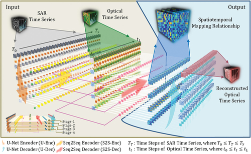
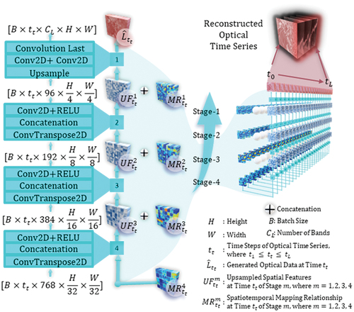
U-SeqNet leveraged a synergy between U-Net and Seq2Seq architectures to establish a robust multimodal spatiotemporal mapping relationship between SAR and optical data (Figure 1). It was conceptualized as a three-dimensional framework with U-Net serving as its backbone. Integrated within this structure were multiple Seq2Seq modules acting as skip connections, effectively bridging the gap between SAR and optical data across both spatial and temporal domains. Upon completion of training, the weights of the U-SeqNet model embodied the acquired spatiotemporal mapping relationship between the optical and SAR time series. When an optical remote sensing time series with missing information was input into the model, the spatiotemporal mapping relationship was utilized to fill in the missing values according to the corresponding SAR time series, thereby obtaining a complete optical remote sensing time series.

Figure 1. Schematic overview of U-SeqNet. The model comprises four key modules: (1) U-Net encoder (U-Enc) for extracting multiscale spatial information (see Section 3.2.1), (2) Seq2Seq encoder (S2S-Enc) for learning temporal features of the spatial information (see Section 3.2.2), (3) Seq2Seq decoder (S2S-Dec) for SAR-to-optical translation (see Section 3.2.3), and (4) U-Net decoder (U-Dec) for utilizing the learned spatiotemporal mapping relationship for reconstruction (see Section 3.2.4). Stage represents different spatial scales.

3.1. Problem formulation

Let $\mathit{L}\in {\mathit{R}}^{t_L\times C_L\times \mathit{H}\times \mathit{W}}$ denote an optical remote sensing time series expressed as a four-dimensional tensor. Here, $t_L$ represents the time steps of the optical remote sensing time series, $C_L$ corresponds to the number of channels, where the channels are the number of bands in the remote sensing image, and $\mathit{H}\times \mathit{W}$ represents the spatial extent characterized by height $\mathit{H}$ and width $\mathit{W}$. Similarly, $\mathit{S}\in {\mathit{R}}^{T_S\times C_S\times \mathit{H}\times \mathit{W}}$ denotes an SAR time series whose time steps and number of bands are represented as $T_S$ and $C_S$ respectively. Additionally, $\mathit{M}\in {\mathit{R}}^{t_L\times 1\times \mathit{H}\times \mathit{W}}$denotes the cloud mask, where 1 indicates pixels with valid observations and 0 indicates missing data values due to cloud coverage. The primary objective of this study was to obtain a complete optical remote sensing time series, denoted as $\hat{L}\in {\mathit{R}}^{t_L\times C_L\times \mathit{H}\times \mathit{W}}$.

3.2. Proposed model

3.2.1. Multiscale spatial information extraction: U-Net encoder with ConvNeXt

The U-Net Encoder module with ConvNeXt in U-SeqNet (hereafter referred to as U-Enc) was specifically designed to extract multiscale spatial information from the input data. U-Enc comprises four stages (Figure 2), each comprising a Downsample layer, followed by a ConvNeXt block using ConvNeXtiny architecture. The downsampling operation included layer normalization (LN) followed by a 2D convolution (Conv2d) layer with a stride (s) and kernel size (k). The ConvNeXt block combined grouped and depthwise separable convolution operations. It consisted of a Depthwise Conv2d layer, LN layer, Conv2d layer with a Gaussian Error Linear Unit (GELU) activation function, and Conv2d layer with layer scaling and a dropout path. The detailed structural parameters of each stage are listed in Table 1.

Figure 2. U-Net encoder (U-Enc) with ConvNeXt in U-SeqNet.

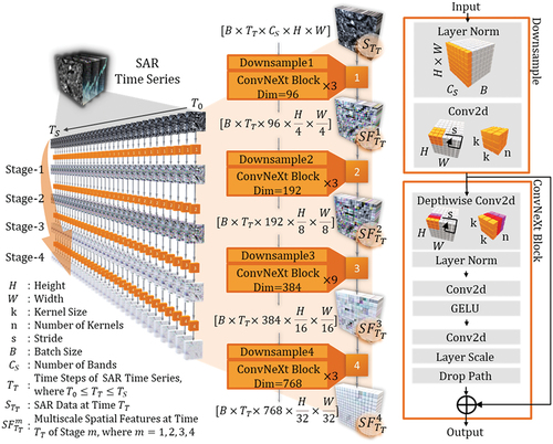
Table 1. Architectural details of the U-Net encoder (U-Enc) with ConvNeXt.

	Kernel Size (k)	Number of Kernels (n)	Stride (s)	Number of Blocks
Downsample1	4×4	96	4	-
ConvNeXt Block Dim = 96	d7×7	96	1	3
	1×1	384
	1×1	96
Downsample2	2×2	192	2	-
ConvNeXt Block Dim = 192	d7×7	192	1	3
	1×1	768
	1×1	192
Downsample3	2×2	384	2	-
ConvNeXt Block Dim = 384	d7×7	384	1	9
	1×1	1536
	1×1	384
Downsample4	2×2	768	2	-
ConvNeXt Block Dim = 768	d7×7	768	1	3
	1×1	3072
	1×1	768

The SAR time series, of dimension ${\mathit{R}}^{T_S\times C_S\times \mathit{H}\times \mathit{W}}$, was processed by the U-Enc to extract multiscale spatial features. Specifically, for each time step $T_T\mathit{\hspace{0.17em}}$($T_0\le T_T\le T_S$), where $S_{T_T}$ represents SAR data at time $T_T$, the U-Enc generates spatial features $\mathit{S}{F}_{T_T}^{\mathit{m}}$ at multiple stages (m = 1, 2, 3, 4), as is illustrated in Figure 2. These stages progressively capture coarser levels of spatial detail. The dimensions of the extracted features at each stage, relative to an input size $\left[\mathit{B}\times T_S\times C_S\times \mathit{H}\times \mathrm{W}\right]$ (where $\mathit{B}$ denotes the batch size), are detailed as follows:

• At Stage-1 ($\mathit{m}=1$), features $\mathit{S}{F}_{T_T}^1$ are of size $\left[\mathit{B}\times T_S\times 96\times \frac{H}{4}\times \frac{W}{4}\right]$;

• At Stage-2 ($\mathit{m}=2$), features $\mathit{S}{F}_{T_T}^2$ are of size $\left[\mathit{B}\times T_S\times 192\times \frac{H}{8}\times \frac{W}{8}\right]$;

• At Stage-3 ($\mathit{m}=3$), features $\mathit{S}{F}_{T_T}^3$ are of size $\left[\mathit{B}\times T_S\times 384\times \frac{H}{16}\times \frac{W}{16}\right]$;

• At Stage-4 ($\mathit{m}=4$), features $\mathit{S}{F}_{T_T}^4$ are of size $\left[\mathit{B}\times T_S\times 768\times \frac{H}{32}\times \frac{W}{32}\right]$.

The outputs of each stage, noted as $\mathit{S}{F}_{T_T}^{\mathit{m}}$, play a crucial role by progressively extracting multiscale spatial information and accurately representing features at different scales. As height and width gradually decrease, U-Enc captures larger-scale spatial patterns and structures, enabling the model to better exploit the spatial information embedded in the remote sensing data.

3.2.2. Spatial information temporal feature learning: Seq2Seq encoder with ConvLSTM

Figure 3(a) illustrates the Seq2Seq architecture within U-SeqNet, which leverages a translation process to handle SAR ($\mathit{Ts}$) and optical ($t_L$) data sequences of varying lengths. The details of this architecture are further elaborated in two sections: Section 3.2.2 focuses on the Seq2Seq Encoder (hereafter referred to as S2S-Enc), while Section 3.2.3 delves into the Seq2Seq Decoder (hereafter referred to as S2S-Dec).

Figure 3. Seq2Seq with ConvLSTM in U-SeqNet. (a) overall structure of U-SeqNet Seq2Seq, with four Seq2Seq modules in each of the four stages for temporal feature learning of multiscale spatial information. (b) internal computations of the ConvLSTM cell. (c)–(e) illustrations of specific inputs and outputs of the ConvLSTM cell.

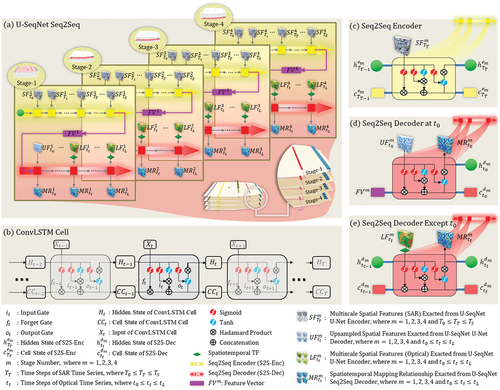
As shown in Figure 3(b), ConvLSTM was utilized during the temporal feature learning process. At time step $\mathit{t}$, the ConvLSTM cell took the current input $X_t$, along with the previously hidden state $H_{\mathit{t}-1}$, and the cell state $\mathit{C}{C}_{\mathit{t}-1}$, as inputs. This produced the current hidden state $H_t$ and cell state $\mathit{C}{C}_t$. The ConvLSTM cell is iterated over time steps thereby enabling effective modeling and learning from the sequences. The update of the hidden state $H_t$ and cell state $\mathit{C}{C}_t$ was controlled by the values of three gates: the input gate $i_t$, forget gate $f_t$, and output gate $o_t$. If the input gate $i_t$ was activated, the input was accumulated in cell state $\mathit{C}{C}_t$. If the forget gate $f_t$ was activated, the previous cell state $\mathit{C}{C}_{\mathit{t}-1}$ was disregarded and the propagation of information from $\mathit{C}{C}_t$ to $H_t$ was regulated by the output gate $o_t$. The specific update steps at time step $\mathit{t}$ were as follows, depicted by equations (1) to (5):

Input gate activation:

(1) $i_t=\mathit{\sigma }\left(W_i*X_t+U_i*H_{\mathit{t}-1}+b_i\right)$(1)

Forget gate activation:

(2) $f_t=\mathit{\sigma }\left(W_f\text{*}{X}_t+U_f\text{*}{H}_{\mathit{t}-1}+b_f\right)$(2)

Cell state update:

(3) $\mathit{C}{C}_t=f_t\otimes \mathit{C}{C}_{\mathit{t}-1}+i_t\otimes \mathit{tanh}\left(W_{\mathit{CC}}*X_t+U_{\mathit{CC}}*H_{\mathit{t}-1}+b_{\mathit{CC}}\right)$(3)

Output gate activation:

(4) $o_t=\mathit{\sigma }\left(W_o*X_t+U_o*H_{\mathit{t}-1}+b_o\right)$(4)

Hidden state update:

(5) $H_t=o_t\otimes \mathit{tanh}\left(\mathit{C}{C}_t\right)$(5)

where $\mathit{\sigma }$ and $\mathit{tanh}$ are activation functions of the sigmoid and hyperbolic tangent, respectively; $\ast$ is the convolution operation; $\otimes$ is the Hadamard product; and $W_i$, $W_f$, $W_o$, $U_i$, $U_f$, $U_o$, $b_i$, $b_f$, and $b_o$ are the learned weights and biases.

As depicted in Figure 3(c), the multiscale spatial features $\mathit{S}{F}_{T_T}^{\mathit{m}}$ extracted by U-Enc are individually fed into the S2S-Enc of each stage. Let $h_{T_T}^{e_m}$ and $c_{T_T}^{e_m}$ represented the hidden state and the cell state of the S2S-Enc at time $T_T$ of stage $\mathit{m}$, respectively. At time step $T_T\mathit{\hspace{0.17em}}$($T_0\le T_T\le T_S$), the spatial features $\mathit{S}{F}_{T_T}^{\mathit{m}}$, the previous hidden state $h_{{\mathit{T}}_{\mathit{T}-1}}^{e_m}$, and the previous cell state $c_{{\mathit{T}}_{\mathit{T}-1}}^{e_m}$ serve as inputs; the current hidden state $h_{T_T}^{e_m}$ and cell state $c_{T_T}^{e_m}$ serve as the outputs. Upon completing the traversal of each time step from $\mathit{S}{F}_{T_0}^{\mathit{m}}$ to $\mathit{S}{F}_{T_S}^{\mathit{m}}$, all hidden and cell states form a feature vector $\mathit{F}{V}^m$. $\mathit{F}{V}^m$ represents the spatial information temporal feature learned by the S2S-Enc at stage $\mathit{m}$.

3.2.3. SAR-to-optical translation: Seq2Seq decoder with ConvLSTM and spatiotemporal TF

To fully leverage the available known information, this study employed spatiotemporal TF, illustrated in Figure 4(a), which enabled the incorporation of all accessible cloud-clear optical imagery with a certain probability as ground truth for the S2S-Dec.

Figure 4. Schematic illustration of spatiotemporal TF. (a) overview of spatiotemporal TF in S2S-Dec. (b) S2S-Dec without spatiotemporal TF. (c) S2S-Dec with spatiotemporal TF.

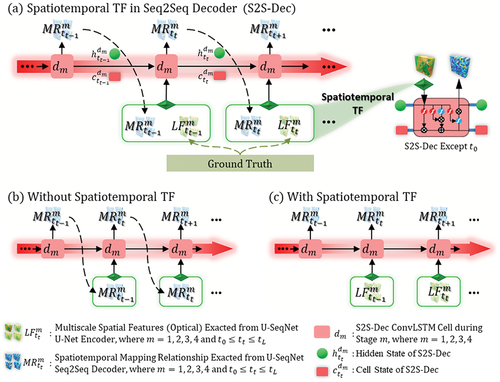
When spatiotemporal TF is absent (0% probability), as shown in Figure 4(b), S2S-Dec relies solely on $\mathit{M}{R}_{{\mathit{t}}_{\mathit{t}-1}}^{\mathit{m}}$ (the previous prediction) to generate $\mathit{M}{R}_{t_t}^{\mathit{m}}$ (the current prediction), and can struggle with convergence and even diverge. In contrast, complete reliance on real values (100% probability), indicated in Figure 4(c), the S2S-Dec depends on $\mathit{L}{F}_{{\mathit{t}}_{\mathit{t}-1}}^{\mathit{m}}$ (the previous ground truth), potentially leading to overfitting. To balance between these extremes, the model incorporates cloud-free real values with a probability of 70% during training, according to equation (6):

(6) $I_{t_t,\mathit{i},\mathit{j}}=\{\mathit{M}{R}_{{\mathit{t}}_{\mathit{t}-1},\mathit{i},\mathit{j}}^{\mathit{m}},\mathit{if}{M}_{t_t,\mathit{i},\mathit{j}}=0\mathit{M}{R}_{{\mathit{t}}_{\mathit{t}-1},\mathit{i},\mathit{j}}^{\mathit{m}},\mathit{if}{M}_{t_t,\mathit{i},\mathit{j}}=1\mathit{AND}\mathit{p}0.3\mathit{L}{F}_{{\mathit{t}}_{\mathit{t}-1},\mathit{i},\mathit{j}}^{\mathit{m}},\mathit{if}{M}_{t_t,\mathit{i},\mathit{j}}=1\mathit{AND}\mathit{p}\ge 0.3$(6)

where, $M_{t_t,\mathit{i},\mathit{j}}$ is the cloud-mask value at pixel $\left(\mathit{i},\mathit{\hspace{0.17em}}\mathit{j}\right)$ and time step $t_t$; and $\mathit{p}$ is a random number between 0 and 1, which determines the output. When $M_{t_t,\mathit{i},\mathit{j}}=0$, indicating the presence of clouds, the input is solely derived from the output $\mathit{M}{R}_{{\mathit{t}}_{\mathit{t}-1},\mathit{i},\mathit{j}}^{\mathit{m}}$ of the previous S2S-Dec. If$M_{t_t,\mathit{i},\mathit{j}}=1$, suggesting a cloud-free scenario, the input variable is set such that there is a 70% chance of incorporating the cloud-free real values $\mathit{L}{F}_{{\mathit{t}}_{\mathit{t}-1},\mathit{i},\mathit{j}}^{\mathit{m}}$ and a 30% chance of reverting to the preceding output $\mathit{M}{R}_{{\mathit{t}}_{\mathit{t}-1},\mathit{i},\mathit{j}}^{\mathit{m}}$ of the S2S-Enc. $\mathit{L}{F}_{t_t}^{\mathit{m}}$, similar to $\mathit{S}{F}_{T_T}^{\mathit{m}}$, is obtained through U-Enc with optical remote sensing time series as input (see Section 3.2.1).

Let $d_m$, $h_{t_t}^{d_m}$, $c_{t_t}^{d_m}$ represent ConvLSTM cell, the hidden states, and cell states of the S2S-Dec at time $t_t$ of stage $\mathit{m}$, respectively. In addition to the inputs previously described, at each time step $t_t\mathit{\hspace{0.17em}}\left(t_1\mathit{\hspace{0.17em}}\le \mathit{\hspace{0.17em}}{t}_t\mathit{\hspace{0.17em}}\le \mathit{\hspace{0.17em}}{t}_L\right)$, as indicated in Figure 3(e), previous hidden state $h_{{\mathit{t}}_{\mathit{t}-1}}^{d_m}$, and cell state $c_{{\mathit{t}}_{\mathit{t}-1}}^{d_m}$ were also used as inputs to the S2S-Dec. S2S-Dec produces the spatiotemporal mapping relationship $\mathit{M}{R}_{t_t}^{\mathit{m}}$, as well as the current hidden state $h_{t_t}^{d_m}$ and cell state $c_{t_t}^{d_m}$.

Furthermore, it is important to note that at the initial time step $t_0$, as indicated in Figure 3(d), the initial input configuration comprised the upsampled spatial features $\mathit{U}{F}_{t_0}^{\mathit{m}}$ extracted from the U-Dec (see Section 3.2.4), combined with the initial hidden state $h_{t_0}^{d_m}$ and the feature vector $\mathit{F}{V}^m$. This configuration is intended to maintain continuity with the $\mathit{F}{V}^m$ learned through the S2S-Enc and to enhance synergy with the following U-Dec.

3.2.4. Reconstruction of optical time series based on the learned spatiotemporal mapping relationship: U-Net decoder

The U-SeqNet U-Net Decoder (hereafter referred to as U-Dec) module was designed to reconstruct optical time series data based on learned spatiotemporal mapping relationships (Figure 5). U-Dec mirrors the structure of U-Enc but in reverse, with four progressively upsampling stages.

Figure 5. U-Net decoder (U-Dec) in U-SeqNet for reconstructing optical time series data based on the learned spatiotemporal mapping relationships.

At time $t_t$, during stages 2–4 of the U-Dec, the operations consist of a ConvTranspose2D, Concatenation, and Conv2D layer followed by a Rectified Linear Unit (ReLU) activation. The input feature map, $\mathit{M}{R}_{t_t}^{\mathit{m}}$, undergoes spatial upscaling through the ConvTranspose2D to produce an upsampled feature map. The concatenation step merged this upsampled map with the original input $\mathit{M}{R}_{t_t}^{\mathit{m}}$, and the subsequent Conv2D plus ReLU layers process the combined features to give the final output $\mathit{U}{F}_{t_t}^{\mathit{m}}$.

At the same time$\mathit{\hspace{0.17em}}{t}_t$ but in stage 1 of U-Dec, a different set of operations is utilized: an Upsample step, followed by two Conv2D layers, and concluding with a Convolutional Last layer. The output differs from stages 2–4, with the final product being the reconstructed time series ${\hat{L}}_{t_t}$. Here, the upsample step was designed to reconstruct fine-grained spatial details, while the Conv2D layers work to capture and refine spatial patterns at a higher resolution. The final convolution, typically involving a 1 × 1 Conv2D, served to collapse the feature maps to the desired number of output channels to produce ${\hat{L}}_{t_t}$.

3.2.5. Loss function

The model was trained by optimizing its parameters through the minimization of the mean squared error (MSE) loss. The MSE loss function, denoted as ${\mathcal{L}}_{\mathit{MSE}}$, was calculated as the average squared difference between the predicted outputs (${\hat{y}}_{\mathit{i}}$) and the ground truth ($y_i$) for the $\mathit{N}$ training samples, as demonstrated by equation (7):

(7) $L_{\mathit{MSE}}=\frac{1}{N}*{\displaystyle {\sum }_{i=1}^N{\left|{\widehat{y}}_{\mathit{i}}-y_i\right|}^2}$(7)

To address the challenge of cloud cover in the dataset for a cloud-prone region, the loss function was refined based on previous work (Peng et al. 2022). The modified loss function $\mathit{L}$ incorporates a cloud mask sequence, defined as $\mathit{M}=\left[M_{1,1,1,1},\dots ,M_{t_t,1,\mathit{i},\mathit{j}},\dots ,M_{t_L,1,\mathit{H},\mathit{W}}\right]\in {\mathit{R}}^{t_L\times 1\times \mathit{H}\times \mathit{W}}$. In this formula,$M_{t_t,1,\mathit{i},\mathit{j}}$ denotes the cloud mask at time $t_t$ for pixel $\left(\mathit{i},\mathit{j}\right)$, with $M_{t_t,1,\mathit{i},\mathit{j}}=1$ indicating clear-sky pixels and $M_{t_t,1,\mathit{i},\mathit{j}}=0$ denoting missing data values due to cloud coverage. Given that $L_{t_t,\mathit{c},\mathit{i},\mathit{j}}$ is the actual observed value and ${\hat{L}}_{t_t,\mathit{c},\mathit{i},\mathit{j}}$ is the predicted value at time $t_t$, $\mathit{c}$-th band, and at pixel $\left(\mathit{i},\mathit{j}\right)$, the adjusted loss function is given by equation (8):

(8) $\mathit{L}=\frac{{\displaystyle \sum _{t_t=1}^{t_L}{\displaystyle \sum _{\mathit{c}=1}^{C_L}{\displaystyle \sum _{\mathit{i}=1}^H{\displaystyle \sum _{\mathit{j}=1}^W{M}_{t_t,1,\mathit{i},\mathit{j}}}}}}{\left|L_{t_t,\mathit{c},\mathit{i},\mathit{j}}-{\widehat{L}}_{t_t,\mathit{c},\mathit{i},\mathit{j}}\right|}^2}{C_L*{\displaystyle \sum _{t_t=1}^{t_L}{\displaystyle \sum _{\mathit{i}=1}^H{\displaystyle \sum _{\mathit{j}=1}^W{M}_{t_t,1,\mathit{i},\mathit{j}}}}}}$(8)

where $C_L$, $t_L$, $\mathit{H}$, and $\mathit{W}$ represents the number of bands, time steps, image height, and width, respectively.

3.3. Evaluation methods

When fully referenced optical images were unavailable for image quality assessment (IQA), three No Reference Image Quality Assessment (NR-IQA) metrics were employed: the Blind/Referenceless Image Spatial Quality Evaluation (BRISQUE) (Mittal, Moorthy, and Bovik 2011, 2012), the Natural Image Quality Evaluator (NIQE) (Mittal, Soundararajan, and Bovik 2013), and the Perceptual Image Quality Evaluator (PIQE) (Venkatanath et al. 2015). BRISQUE utilizes natural scene statistics to measure image distortion and offers a universal distortion measure, whereby lower BRISQUE scores indicate better image quality. NIQE compares image quality based on natural scene statistics and is a reference model for evaluating image quality, with lower NIQE scores indicating better image quality. Similarly, PIQE assesses image quality based on perceptual characteristics, considered various perceptual aspects, and provides insights into the visual quality of images. Lower PIQE scores indicated better image quality.

In cases where the reference images contain clear pixels, additional Full-Reference Image Quality Assessment (FR-IQA) techniques were adopted for quantitative evaluation, namely: the Mean Absolute Error (MAE) (Cort and Kenji 2005), Mean Squared Error (MSE) (Wang and Bovik 2009), Peak Signal-to-Noise Ratio (PSNR) (Sebastianelli et al. 2022), and Structural Similarity Index Measure (SSIM) (W. Zhou et al. 2004). These metrics objectively measure the discrepancy between generated and reference images. Lower MAE and MSE values indicate improved image quality. Higher PSNR values corresponded to better image quality. Higher SSIM values indicated better structural similarity. MAE, MSE, PSNR, and SSIM were calculated using real values ($\mathit{y}$), and generated values, ($\hat{y}$) as follows, depicted by equations (9) to (12):

(9) $\mathit{MAE}=\frac{1}{N}{\displaystyle \sum _{\mathit{i}=1}^N\left|y_i-{\widehat{y}}_{\mathit{i}}\right|}$(9)

(10) $\mathit{MSE}=\frac{1}{N}{\displaystyle \sum _{\mathit{i}=1}^N{\left(y_i-{\widehat{y}}_{\mathit{i}}\right)}^2}$(10)

(11) $\mathit{PSNR}=10\cdot {\mathit{log}}_{10}\left(\frac{MA{X}_I^2}{\mathit{MSE}}\right)$(11)

(12) $\mathit{SSIM}\left(\mathit{y},\widehat{y}\right)=\frac{\left(2{\mu }_y{\mu }_{\widehat{y}}+c_1\right)\left(2{\sigma }_{y,\widehat{y}}+c_2\right)}{\left({\mu }_y^2+{\mu }_{\widehat{y}}^2+c_1\right)\left({\sigma }_y^2+{\sigma }_{\widehat{y}}^2+c_2\right)}$(12)

where, $\mathit{y}$, $\hat{y}$, and $\mathit{N}$ denotes real values, generated values, and total number of samples, respectively; $\mathit{MA}{X}_I$ is the maximum possible pixel value of the image; ${\mu }_y$ and ${\mu }_{\hat{y}}$ are the average of $\mathit{y}$ and $\hat{y}$, respectively; ${\sigma }_y^2$ and ${\sigma }_{\hat{y}}^2$ are the variance of $\mathit{y}$ and $\hat{y}$, respectively; ${\sigma }_{y,\hat{y}}$ is the covariance of $\mathit{y}$ and $\hat{y}$; $c_1=\begin{array}{c}\mathit{\hspace{0.17em}}{\left(k_1\mathit{R}\right)}^2\end{array}$ and $c_2=\begin{array}{c}\mathit{\hspace{0.17em}}{\left(k_2\mathit{R}\right)}^2\end{array}$ are two variables employed to stabilize the division process with a weak denominator; $\mathit{R}$ is the dynamic range of the pixel-values, and $k_1=\mathit{\hspace{0.17em}}0.01$ and $k_2=\mathit{\hspace{0.17em}}0.03$ by default.

4. Experiments

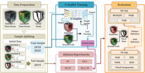
The experimental procedure comprised several steps (Figure 6). Initially, the data preparation stage involved acquiring SAR time series data from Sentinel-1 and optical time series data from Landsat 8. Subsequently, the collected data were divided into training and testing sets. The next step involved training the U-SeqNet model. The training data were fed into the proposed model and through iterative calculations of the loss function and weight updates, the model was trained until convergence was achieved, resulting in the final model state. Following the training phase, ablation experiments were performed. Four sets of experiments were designed (see Section 4.2) to evaluate the performance of the proposed model under different configurations. The optical time series data generated from these experiments were then assessed for accuracy.

Figure 6. Flow diagram showing the experimental procedure for U-SeqNet-based SAR-to-optical image translation and evaluation.

4.1. Data and preparation

4.1.1. Optical time series from landsat 8

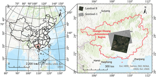
Landsat 8, equipped with an operational land imager and thermal infrared sensor, offers a spatial resolution of 30 m and a temporal resolution of 16 days. A dataset comprising 66 level-two surface reflectance images covering the time span from 2018 to 2020 was acquired from path/row 125/44, which corresponds to a study area centered on Guangxi, China (Figure 7). This area, situated between 22° and 24° N and 108° to 110° E, has a subtropical to tropical climate with heavy rainfall, complicating the acquisition of cloud-free images. Data were obtained from the United States Geological Survey (USGS). A mask function (Fmask) (Z. Zhu, Wang, and Woodcock 2015; Z. Zhu and Woodcock 2012) was employed to identify cloudy regions within the Landsat 8 data and generate a corresponding cloud mask. Fmask allows for the detection and labeling of invalid cloud regions, enabling users to differentiate between areas affected and unaffected by clouds.

Figure 7. Study area.

4.1.2. SAR time series from sentinel-1

Sentinel-1 is a constellation composed of the Sentinel-1A and Sentinel-1B satellites equipped with a C-SAR instrument designed for reliable large-scale monitoring. Sentinel-1 is an all-weather radar-imaging system that operates continuously. Within the spatiotemporal extent corresponding to Landsat 8 (Figure 7), 92 Level-1 ground-range-detected high-resolution images were acquired from the European Space Agency (ESA), covering the period from 2018 to 2020. All images were acquired during ascending Sentinel-1A passes. The ground-range-detected high-resolution product was acquired in interferometric wide mode with dual polarization (VH and VV), providing a spatial resolution of 5 × 20 m and a revisit frequency of 12 days. As Sentinel-1 and Landsat 8 are independent imaging systems, their spatial positions and resolutions differ. Hence, geocoding and resampling processes, with a final resampled resolution of 30 m, were required to adjust the dataset alignment (see (Peng et al. 2022), Section III.B.2 for the detailed procedures).

4.2. Experimental settings

To validate the performance of ConvNeXt and the spatiotemporal TF, the following ablation experiments were conducted (Table 2).

Table 2. Utilization of ConvNeXt and spatiotemporal TF in ablation experiments.

Experiment	Utilization of ConvNeXt	Utilization of Spatiotemporal TF
Experiment 1 (US)	No	No
Experiment 2 (US_C)	Yes	No
Experiment 3 (US_TF)	No	Yes
Experiment 4 (US_C_TF)	Yes	Yes

All experiments were conducted using heterogeneous node 4D1, which consisted of four heterogeneous accelerator cards, an X86 7185 32C 2.0-GHz CPU, 128-GB memory, and 200-Gb computing network. Experiments were conducted using the PyTorch framework in Python. Based on the debugging results, the following hyperparameters were used: Adam optimizer, learning rate of 0.001, and batch size of 2.

4.3. Model training

During the training phase, the model used 1,692 training pairs measuring 256 × 256 pixels derived from Sentinel-1, Landsat 8, and cloud mask data collected in 2018 and 2020 to synthesize generated Landsat 8 images. This training process adhered to the loss function protocol (see Section 3.2.5). During the testing phase, the model used 846 test pairs derived from 2019 data.

In accordance with the mathematical definitions (see Section 3.1), the cloud mask data dimensions were noted as 22 × 1 × 256 × 256. The dimensions for the input Landsat 8 and generated Landsat 8 data were established at 22 × 6 × 256 × 256, where “22” corresponds to the number of Landsat 8 images acquired annually and “6” represents the six spectral bands, namely, blue, green, red, Near-InFrared (NIR), ShortWave InFrared 1 (SWIR1), and ShortWave InFrared 2 (SWIR2). The dimensions of Sentinel-1 input data were specified as 31 × 2 × 256 × 256 during the training phase and 30 × 2 × 256 × 256 during the testing phase. This discrepancy was attributed to the annual variation in the number of images acquired by Sentinel-1: “31” for the years 2018 and 2020, and “30” for 2019, with “2” representing the two polarization bands, VV and VH.

5. Results

5.1. Image quality assessment without a reference

For the evaluation using NR – IQA metrics, the BRISQUE, NIQE, and PIQE were utilized (Table 3). In the BRISQUE evaluation, the US_C_TF experiment achieved the lowest BRISQUE scores in the blue, red, NIR, SWIR1, and SWIR2 bands, indicating a relatively higher image quality when both ConvNeXt and spatiotemporal TF were combined. The US_TF experiment exhibited the best BRISQUE score in the green band and comparable performance to US_C_TF in the blue, red, NIR, and SWIR2 bands.

Table 3. Quantitative assessment of quality of reconstruction without using a reference image.

	Experiment	Blue	Green	Red	NIR	SWIR1	SWIR2	Average
BRISQUE↓	US	46.21	46.43	46.29	47.13	44.76	44.49	45.88
	US_C	45.50	44.88	44.90	45.06	44.65	40.89	44.31
	US_TF	44.49	44.45	44.47	44.52	44.76	40.40	43.85
	US_C_TF	44.43	44.46	44.46	44.50	44.62	38.93	43.57
NIQE↓	US	10.10	9.81	10.35	12.42	12.20	12.03	11.15
	US_C	4.87	4.87	4.61	12.34	5.38	4.77	6.14
	US_TF	4.61	4.70	4.60	11.33	5.63	5.28	6.02
	US_C_TF	4.32	4.40	4.33	12.14	4.86	5.06	5.85
PIQE↓	US	69.04	74.89	64.27	90.00	79.81	56.13	72.36
	US_C	53.76	49.29	48.57	87.50	67.44	48.27	59.14
	US_TF	50.85	47.56	51.27	89.32	64.06	46.32	58.23
	US_C_TF	40.74	31.64	32.82	81.16	40.50	25.63	42.08

Regarding the NIQE evaluation, the US_C_TF experiment yielded the lowest NIQE scores in the blue, green, red, and SWIR1 bands, implying better image quality when both ConvNeXt and spatiotemporal TF were employed. Except for the NIR band, significant NIQE reductions were observed regardless of the use of ConvNeXt or spatiotemporal TF, with average improvements of 5.01 and 5.13, corresponding to enhancements of 44.92% and 45.99%, respectively. These findings indicate that both ConvNeXt and spatiotemporal TF contributed to closer alignment between the reconstructed images and the statistical characteristics of the natural images.

In the PIQE evaluation, US_C_TF achieved the lowest PIQE scores across all bands. Similar to NIQE, substantial PIQE reductions were observed in all bands, except NIR, when employing either ConvNeXt or spatiotemporal TF. This suggests that both ConvNeXt and spatiotemporal TF enhanced the perceived characteristics of the reconstructed images, including brightness, contrast, and color saturation, resulting in greater correspondence with the characteristics of natural images.

In conclusion, the BRISQUE, NIQE, and PIQE metrics revealed that the US_C_TF experiment, which combined ConvNeXt and spatiotemporal TF, consistently outperformed or ranked second-best across all bands, indicating its positive influence on enhancing image quality. This combined approach improved the spatial, statistical, and perceptual qualities of the generated images. Observations indicate that the NIR band experienced relatively lower performance in both NIQE and PIQE metrics. This pattern warrants further investigation to determine underlying factors specific to the NIR band that may affect image reconstruction quality.

5.2. Image quality assessment with a reference

Qualitative and quantitative evaluations of image outputs are detailed in Figure 8 and Table 4, respectively. Visual comparisons and objective assessments via FR-IQA metrics (MAE, MSE, PSNR, and SSIM) were compared.

Figure 8. Comparison of generated results with ground truth data: (a) ground truth - landsat 8 image from December 5, 2019. Generated images from different ablation experiments: (b) US, (c) US_C, (d) US_TF, and (e) US_C_TF.

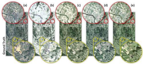
Table 4. Quantitative assessment of quality of reconstruction using a reference image.

Experiment	MAE↓	MSE↓	PSNR↑	SSIM↑
US	0.0692	0.0146	18.3705	0.5343
US_C	0.0464	0.0073	21.3744	0.8072
US_TF	0.0407	0.0048	23.1749	0.7869
US_C_TF	0.0391	0.0046	23.3300	0.8119

The control experiment (US) yielded the least satisfactory visual quality and only achieved image reconstruction. However, when ConvNeXt alone introduced (US_C), the generated images demonstrated an improvement in textural details, particularly regarding continuity of the river boundaries (indicated by the red circle in Figure 8). However, the inclusion of spatiotemporal TF alone (US_TF) resulted in generated images that exhibited a closer resemblance to the ground truth in terms of overall color tones. Notably, the experiment combining ConvNeXt and spatiotemporal TF (US_C_TF) achieved even closer visual quality to the ground truth. This is evident in the representation of internal urban structures (indicated by the red circle in Figure 8) and fidelity of mountain shadow intensity (indicated by the yellow circle in Figure 8).

The US experiment exhibited the lowest visual quality, as indicated by its highest MAE and MSE values and lowest PSNR and SSIM values (Table 4). In contrast, the US_C experiment showed a notable improvement in the generated images. The SSIM value increased from 0.5343 to 0.8072, reaching a comparable level to the US_C_TF experiment. In addition, the US_TF experiment achieved similar performance to US_C_TF, with almost equal PSNR values (23.1749 for US_TF and 23.3300 for US_C_TF). The US_C_TF experiment achieved the lowest MAE and MSE values and the highest PSNR and SSIM values among all experiments, indicating a higher similarity to the ground truth image.

6. Discussion

6.1. Image quality under mixed cloud conditions

Previous research has demonstrated the use of simulated cloudy conditions for the evaluation of the quality of reconstructed images in remote sensing (Xia and Jia 2022). Such studies often leverage FR-IQA metrics like SSIM, PSNR, and MSE (Kaur, Koundal, and Kadyan 2021; Kulkarni and Rege 2020). While this study did not employ artificial cloud masking, recognizing its potential utility in representing mixed cloud conditions in remote sensing datasets is imperative.

In this study, a two-pronged approach was taken to handle different conditions. For cloud-free regions, FR – IQA metrics (SSIM, PSNR, MAE, and MSE) were employed. The SSIM metric was calculated using a standardized sliding window technique across areas exceeding 125 × 125 pixels. PSNR, MAE, and MSE were based on all available cloud-free pixels. However, for cloud contamination regions, a suite of NR – IQA metrics (BRISQUE, UIQE, and PIQE) was applied. However, these metrics were traditionally developed for natural image assessment and may not fully align with the distinctive characteristics of remote sensing data. This could explain why the PIQE exceeded 70, indicating poor performance. Nonetheless, these metrics are critical for assessing cloud contamination regions where ground truth is not available, enabling a wide-ranging evaluation of image quality.

6.2. Cloud ratio impact on U-SeqNet performance

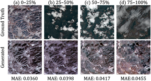
The impact of cloud ratio on cloud removal techniques has garnered considerable research attention (F. Xu et al. 2022). This study further assessed the performance of U-SeqNet under varying levels of cloudiness. In low-cloud scenarios (0%–25%), U-SeqNet excelled (Figure 9), evidenced by low MAE. However, as cloud cover intensified (75%–100%), its accuracy declined, revealing the negative impact of cloud cover on U-SeqNet.

Figure 9. Comparison of ground truth and generated imagery across varying cloud ratios: (a) 0–25% cloud coverage, (b) 25–50% cloud coverage, (c) 50–75% cloud coverage, and (d) 75–100% cloud coverage. The size of each image is 256 × 256 pixels.

6.3. Interpolation and extrapolation efficacy

Time series reconstruction typically entails both interpolation and extrapolation scenarios (Jhin et al. 2022). This study utilized remote-sensing data from 2018 to 2020 for model training, with the intermediate year 2019 serving as the test case. This strategy validates the model’s prowess in interpolation. Nonetheless, the extrapolation capabilities, which would involve making predictions for data points outside the training period (e.g. using data from 2018 to 2019 to forecast results for 2020), remain untested within the current framework. The challenge of extrapolation assumes greater importance in contexts where later images might not be available, a factor that could impinge on the generalizability and practical applicability of the research outcomes. Future research may benefit from considering extended datasets and time ranges to fully explore the extrapolation capabilities of time series reconstruction models.

6.4. Spatial transferability of U-SeqNet

The concern for spatial transferability is paramount in the practical deployment of remote sensing models. U-SeqNet’s innovative amalgamation of U-Net and Seq2Seq architectures underlines its adaptability, enabling it to harness and interpret the ubiquitous spatiotemporal relationships found within multisource satellite data.

Firstly, U-SeqNet’s unique proposition stems from its ability to merge U-Net’s spatial mapping proficiency with Seq2Seq’s temporal modeling capabilities. This fusion effectively captures the widespread spatiotemporal patterns that are fundamental to remote sensing data. Such synergy not only bolsters the model’s competence in addressing multimodal and multitemporal cloud removal challenges but also facilitates the learning and simulation of complex spatiotemporal dynamics across diverse geographic landscapes. Secondly, U-SeqNet’s emphasis on assimilating the inherent spatiotemporal attributes of remote sensing data, as opposed to location-specific features, significantly enhances its spatial transferability. This strategy ensures the model’s utility across different satellite imagery by leveraging universal attributes, thereby promising robust spatial applicability. Consequently, given that the foundational properties and structures of the remote sensing data remain consistent, U-SeqNet is poised to perform effectively in a myriad of geographical contexts.

6.5. Model comparative analysis and future directions for U-SeqNet improvement

In response to concerns about the validation of U-SeqNet, a comparative analysis was conducted with other models, namely Improved Seq2Seq (Peng et al. 2022) and UnCRtainTS (Ebel et al. 2023). The study employed NR-IQA and FR-IQA metrics for evaluation (Table 5). U-SeqNet outperformed the other models for on every metric.

Table 5. Quantitative comparison of U-SeqNet with other models.

	NR-IQA			FR-IQA
	BRISQUE↓	NIQE↓	PIQE↓	MAE↓	MSE↓	PSNR↑	SSIM↑
Improved Seq2Seq	46.70	6.39	61.42	0.0465	0.0072	21.45	0.67
UnCRtainTS	45.70	6.38	49.50	0.0433	0.0062	22.07	0.74
U-SeqNet	43.57	5.85	42.08	0.0391	0.0046	23.33	0.81

In addition to the comparative results with other models, the four ablation experiments also demonstrate that the novel combination of spatiotemporal TF and ConvNeXt achieves an advanced level and is capable of completing the reconstruction task. However, the magnitude of the improvement did not meet expectations, a matter attributable to a few key factors. Specifically, the large number of time steps in the target reconstruction sequence led to learned context vectors in the S2S-Enc being discarded in subsequent stages of the S2S-Dec and U-Dec. This is because the latter two components focus on the target reconstruction sequence. Compounded by this, the repeated updates of hidden and cell states in ConvLSTM, driven by extensive time steps, may weaken the effectiveness of the context vectors. Moreover, concerns regarding color fidelity underscore the necessity for an enriched exploration of spectral information within training processes.

The future trajectory of research is poised to embark on a deepened analysis of strategies to enhance reconstructions. One potential avenue for improvement is to determine the optimal number of time steps. Given the revisit characteristics of satellite imagery, in which images captured at different times within a significant time span are available for the same location, notable differences in appearance were observed, including seasonal variation and variations in lighting and weather conditions. In remote sensing, seasonal contrastive learning has been proposed to enable models to learn and extract season-invariant features (MañMañAs et al. 2021). Inspired by the work time series length effect (Stucker, Garnot, and Schindler 2023), there is an inclination to assess the potential of a multisensory encoder configuration. By dividing the annual time series into four seasons and employing four encoders to obtain four context vectors, relevant temporal information can be captured, thereby enhancing the reconstruction performance and mitigating the adverse effects of excessive time steps. In consideration of color fidelity, future work should meticulously design processing techniques that preserve the distinct spectral information present across different bands. The incorporation of channel attention mechanisms could be pivotal, as such approaches selectively enhance critical features while suppressing less informative ones, maintaining the intricate spectral signatures that are essential for accurate remote sensing analysis.

7. Conclusion

In this study, a novel model, U-SeqNet, which combines U-Net and Seq2Seq architectures was developed to address the challenges of SAR-to-optical image translation. By utilizing ConvNeXt as the U-Net backbone and ConvLSTM as the Seq2Seq kernel, along with spatiotemporal TF, U-SeqNet demonstrates promising capabilities. The main conclusions of this study are as follows: (1) The U-SeqNet architecture, which combines U-Net and Seq2Seq architectures, demonstrates effective performance in extracting spatiotemporal information and successfully performing optical time series reconstruction tasks. (2) Quantitative evaluations of image quality without a reference image utilized BRISQUE, NIQE, and PIQE metrics. The evaluation results indicated that U-SeqNet, significantly improves the spatial characteristics, statistical properties, and perceptual quality of the generated images. Notably, the performance of the proposed method in the NIR band, as assessed by NIQE and PIQE metrics, was relatively poor. This limitation can be attributed to the considerable spectral variation in land features within this band, which poses challenges for the reconstruction process. (3) Quantitative evaluations of image quality with a reference image, which used metrics such as MAE, MSE, PSNR, and SSIM along with visual inspection, further supported the effectiveness of U-SeqNet. The proposed method achieved the best visual quality for image reconstruction. Moreover, the combination of ConvNeXt and spatiotemporal TF exhibited notable improvements in the texture detail, overall tone, and fidelity of generated images.

These findings provide a foundation for enhancing synchronization in cloud removal and data reconstruction by effectively extracting spatiotemporal information. Although this study focused on translating Sentinel-1 data to the Landsat 8 time series, reconstructing other SAR time series into optical time series is theoretically feasible. The proposed model offers valuable insights into the application of deep learning techniques for spatiotemporal analysis in remote sensing. These findings contribute to the development of more efficient and accurate multimodal, multitemporal cloud removal methods. In future research, it will be essential to develop reconstruction metrics for scenarios where reference data are unavailable, as well as adaptive multi-encoder approaches to incorporate seasonal information and further enhance reconstruction accuracy. These advances will further enhance the quality and precision of reconstructed time series data.

Acknowledgments

This research was funded by the National Natural Science Foundation of China under Grant 41871223. We gratefully acknowledge the USGS for providing Landsat data and the ESA for providing Sentinel-1 data. Additionally, we would like to thank Sugon (www.sugon.com) for providing the data computing services at the Hefei Advanced Computing Center. We would also like to thank Editage (www.editage.com) for English language editing.

Disclosure statement

The authors declare that they have no known competing financial interests or personal relationships that could have appeared to influence the work reported in this paper.

Data availability statement

The model of this study is available on GitHub at https://github.com/lexyzhang/U-SeqNet/tree/main.

Additional information

Funding

The work was supported by the National Natural Science Foundation of China under Grant [41871223].

References

- Bermudez, J. D., P. N. Happ, D. A. B. Oliveira, and R. Q. Feitosa. 2018. “SAR to Optical Image Synthesis for Cloud Removal with Generative Adversarial Networks.” Paper presented at the ISPRS TC I Mid-term Symposium on Innovative Sensing - From Sensors to Methods and Applications, Karlsruhe, GERMANY.
- Cheng, Q., H. Shen, L. Zhang, Q. Yuan, and C. Zeng. 2014. “Cloud Removal for Remotely Sensed Images by Similar Pixel Replacement Guided with a Spatio-Temporal MRF Model.” ISPRS Journal of Photogrammetry and Remote Sensing 92:54–19. https://doi.org/10.1016/j.isprsjprs.2014.02.015.
- Cort, J. W., and M. Kenji. 2005. “Advantages of the Mean Absolute Error (MAE) Over the Root Mean Square Error (RMSE) in Assessing Average Model Performance.” Climate Research 30 (1): 79–82. https://doi.org/10.3354/cr030079.
- Ding, H., F. Xie, Y. Zi, W. Liao, and X. Song. 2023. “Feedback Network for Compact Thin Cloud Removal.” Geoscience and Remote Sensing Letters, IEEE 20:1–5. https://doi.org/10.1109/LGRS.2023.3256416.
- Ebel, P., V. S. Fare Garnot, M. Schmitt, J. D. Wegner, and X. Xiang Zhu. 2023. “UnCrtainTS: Uncertainty Quantification for Cloud Removal in Optical Satellite Time Series.” Paper presented at the 2023 IEEE/CVF Conference on Computer Vision and Pattern Recognition Workshops (CVPRW), Vancouver, BC, Canada.
- Ebel, P., M. Schmitt, and X. X. Zhu. 2021. “Internal Learning for Sequence-To-Sequence Cloud Removal via Synthetic Aperture Radar Prior Information.” Paper presented at the 2021 IEEE International Geoscience and Remote Sensing Symposium IGARSS, Brussels, Belgium.
- Ebel, P., Y. Xu, M. Schmitt, and X. Xiang Zhu. 2022. “Sen12MS-CR-TS: A Remote-Sensing Data Set for Multimodal Multitemporal Cloud Removal.” IEEE Trans. Geosci. Remote Sens. 60. https://doi.org/10.1109/tgrs.2022.3146246.
- Friedl, M. A., D. K. McIver, J. C. F. Hodges, X. Y. Zhang, D. Muchoney, A. H. Strahler, C. E. Woodcock, et al. 2002. “Global Land Cover Mapping from MODIS: Algorithms and Early Results.” Remote Sensing of Environment 83 (1–2): 287–302. https://doi.org/10.1016/s0034-4257(02)00078-0.
- Ghamisi, P., B. Rasti, N. Yokoya, Q. Wang, B. Hoefle, L. Bruzzone, F. Bovolo, et al. 2019. “Multisource and Multitemporal Data Fusion in Remote Sensing a Comprehensive Review of the State of the Art.” IEEE Transactions on Geoscience and Remote Sensing: A Publication of the IEEE Geoscience and Remote Sensing Society 7 (1): 6–39. https://doi.org/10.1109/mgrs.2018.2890023.
- Goodfellow, I. J., J. Pouget-Abadie, M. Mirza, B. Xu, D. Warde-Farley, S. Ozair, A. Courville, and Y. Bengio. 2014. “Generative adversarial nets.” In Proceedings of the 27th International Conference on Neural Information Processing Systems, 2672–2680. Montreal, Canada: MIT Press.
- Hochreiter, S., and J. Schmidhuber. 1997. “Long Short-Term Memory.” Neural Computation 9 (8): 1735–1780. https://doi.org/10.1162/neco.1997.9.8.1735.
- Jhin, S. Y., J. Lee, M. Jo, S. Kook, J. Jeon, J. Hyeong, J. Kim, and N. Park. 2022. “EXIT: Extrapolation and Interpolation-Based Neural Controlled Differential Equations for Time-Series Classification and Forecasting.” In Proceedings of the ACM Web Conference 2022, 3102–3112. Virtual Event, Lyon, France: Association for Computing Machinery.
- Ji, S., S. Wei, and M. Lu. 2019. “Fully Convolutional Networks for Multisource Building Extraction from an Open Aerial and Satellite Imagery Data Set.” IEEE Transactions on Geoscience and Remote Sensing: A Publication of the IEEE Geoscience and Remote Sensing Society 57 (1): 574–586. https://doi.org/10.1109/tgrs.2018.2858817.
- Kaur, H., D. Koundal, and V. Kadyan. 2021. “Image Fusion Techniques: A Survey.” Archives of Computational Methods in Engineering 28 (7): 4425–4447. https://doi.org/10.1007/s11831-021-09540-7.
- Kulkarni, S. C., and P. P. Rege. 2020. “Pixel level fusion techniques for SAR and optical images: A review.” Information Fusion 59:13–29. https://doi.org/10.1016/j.inffus.2020.01.003.
- LeCun, Y., B. Boser, J. S. Denker, D. Henderson, R. E. Howard, W. Hubbard, and L. D. Jackel. 1989. “Backpropagation Applied to Handwritten Zip Code Recognition.” Neural Computation 1 (4): 541–551. https://doi.org/10.1162/neco.1989.1.4.541.
- Li, X., Z. Du, Y. Huang, and Z. Tan. 2021. “A Deep Translation (GAN) Based Change Detection Network for Optical and SAR Remote Sensing Images.” ISPRS Journal of Photogrammetry and Remote Sensing 179:14–34. https://doi.org/10.1016/j.isprsjprs.2021.07.007.
- Li, J., D. Hong, L. Gao, J. Yao, K. Zheng, B. Zhang, and J. Chanussot. 2022. “Deep Learning In Multimodal Remote Sensing Data Fusion: A Comprehensive Review.” International Journal of Applied Earth Observation and Geoinformation 112. https://doi.org/10.1016/j.jag.2022.102926.
- Lin, C.-H., P.-H. Tsai, K.-H. Lai, and J.-Y. Chen. 2013. “Cloud Removal from Multitemporal Satellite Images Using Information Cloning.” IEEE Transactions on Geoscience and Remote Sensing: A Publication of the IEEE Geoscience and Remote Sensing Society 51 (1): 232–241. https://doi.org/10.1109/tgrs.2012.2197682.
- Liu, L., and B. Lei. 2018. “Can SAR Images and Optical Images Transfer with Each Other?.” Paper presented at the 38th IEEE International Geoscience and Remote Sensing Symposium (IGARSS), Valencia, SPAIN.
- Liu, Z., H. Mao, C. Y. Wu, C. Feichtenhofer, T. Darrell, and S. Xie. 2022. ”A ConvNet for the 2020s.” Paper presented at the 2022 IEEE/CVF Conference on Computer Vision and Pattern Recognition (CVPR), New Orleans, LA, USA.
- Li, Y., F. Wei, Y. Zhang, W. Chen, and J. Ma. 2023. “HS2P: Hierarchical Spectral and Structure-Preserving Fusion Network for Multimodal Remote Sensing Image Cloud and Shadow Removal.” Information Fusion 94:215–228. https://doi.org/10.1016/j.inffus.2023.02.002.
- Ma, L., Y. Liu, X. Zhang, Y. Ye, G. Yin, and B. Alan Johnson. 2019. “Deep Learning in Remote Sensing Applications: A Meta-Analysis and Review.” ISPRS Journal of Photogrammetry and Remote Sensing 152:166–177. https://doi.org/10.1016/j.isprsjprs.2019.04.015.
- MañMañAs, O., A. Lacoste, X. Giró-I-Nieto, D. Vázquez, and P. Rodriguez. 2021. “Seasonal Contrast: Unsupervised Pre-Training from Uncurated Remote Sensing Data.” In 2021 IEEE/CVF International Conference on Computer Vision (ICCV), Montreal, QC, Canada, 9394–9403. IEEE Computer Society.
- Ma, D., R. Wu, D. Xiao, and B. Sui. 2023. “Cloud Removal from Satellite Images Using a Deep Learning Model with the Cloud-Matting Method.” Remote Sensing 15:4. https://doi.org/10.3390/rs15040904.
- Meraner, A., P. Ebel, X. Xiang Zhu, and M. Schmitt. 2020. “Cloud removal in Sentinel-2 imagery using a deep residual neural network and SAR-optical data fusion.” ISPRS Journal of Photogrammetry and Remote Sensing 166:333–346. https://doi.org/10.1016/j.isprsjprs.2020.05.013.
- Mittal, A., A. K. Moorthy, and A. C. Bovik. 2011. “Blind/Referenceless Image Spatial Quality Evaluator.” Paper presented at the 2011 Conference Record of the Forty Fifth Asilomar Conference on Signals, Systems and Computers (ASILOMAR), Pacific Grove, CA, USA.
- Mittal, A., A. K. Moorthy, and A. C. Bovik. 2012. “No-Reference Image Quality Assessment in the Spatial Domain.” IEEE Transactions on Image Processing 21 (12): 4695–4708. https://doi.org/10.1109/TIP.2012.2214050.
- Mittal, A., R. Soundararajan, and A. C. Bovik. 2013. “Making a “Completely Blind” Image Quality Analyzer.” IEEE Signal Processing Letters 20 (3): 209–212. https://doi.org/10.1109/LSP.2012.2227726.
- Papadomanolaki, M., M. Vakalopoulou, and K. Karantzalos. 2021. “A Deep Multitask Learning Framework Coupling Semantic Segmentation and Fully Convolutional LSTM Networks for Urban Change Detection.” IEEE Transactions on Geoscience and Remote Sensing: A Publication of the IEEE Geoscience and Remote Sensing Society 59 (9): 7651–7668. https://doi.org/10.1109/tgrs.2021.3055584.
- Pekel, J.-F., A. Cottam, N. Gorelick, and A. S. Belward. 2016. “High-Resolution Mapping of Global Surface Water and Its Long-Term Changes.” Nature 540 (7633): 418±. https://doi.org/10.1038/nature20584.
- Peng, T., M. Liu, X. Liu, Q. Zhang, L. Wu, and X. Zou. 2022. “Reconstruction of Optical Image Time Series with Unequal Lengths SAR Based on Improved Sequence-Sequence Model.” IEEE Trans. Geosci. Remote Sens. 60. https://doi.org/10.1109/tgrs.2022.3208926.
- Reyes, M. F., S. Auer, N. Merkle, C. Henry, and M. Schmitt. 2019. “SAR-To-Optical Image Translation Based on Conditional Generative Adversarial Networks-Optimization, Opportunities and Limits.” Remote Sensing 11 (17). https://doi.org/10.3390/rs11172067.
- Ronneberger, O., P. Fischer, and T. Brox. 2015. “U-Net: Convolutional Networks for Biomedical Image Segmentation.” Paper presented at the Medical Image Computing and Computer-Assisted Intervention – MICCAI 2015, Cham.
- Rumelhart, D. E., G. E. Hinton, and R. J. Williams. 1986. “Learning Representations by Back-Propagating Errors.” Nature 323 (6088): 533–536. https://doi.org/10.1038/323533a0.
- Sangiorgio, M., and F. Dercole. 2020. “Robustness of LSTM Neural Networks for Multi-Step Forecasting of Chaotic Time Series.” Chaos, Solitons & Fractals 139. https://doi.org/10.1016/j.chaos.2020.110045.
- Schmitt, M., L. Hughes, and X. Zhu. 2018. “The SEN1-2 Dataset For Deep Learning In Sar-optical Data Fusion.” ISPRS Annals of Photogrammetry, Remote Sensing & Spatial Information Sciences IV-1: 141–146. https://doi.org/10.5194/isprs-annals-IV-1-141-2018.
- Sebastianelli, A., E. Puglisi, M. Pia Del Rosso, J. Mifdal, A. Nowakowski, P. Philippe Mathieu, F. Pirri, and S. Liberata Ullo. 2022. “PLFM: Pixel-Level Merging of Intermediate Feature Maps by Disentangling and Fusing Spatial and Temporal Data for Cloud Removal.” IEEE Transactions on Geoscience and Remote Sensing: A Publication of the IEEE Geoscience and Remote Sensing Society 60:1–16. https://doi.org/10.1109/tgrs.2022.3208694.
- Shen, H., X. Li, Q. Cheng, C. Zeng, G. Yang, H. Li, and L. Zhang. 2015. “Missing Information Reconstruction of Remote Sensing Data: A Technical Review.” IEEE Transactions on Geoscience and Remote Sensing: A Publication of the IEEE Geoscience and Remote Sensing Society 3 (3): 61–85. https://doi.org/10.1109/mgrs.2015.2441912.
- Shi, X., Z. Chen, H. Wang, D.-Y. Yeung, W.-K. Wong, and W.-C. Woo. 2015. “Convolutional LSTM Network: A Machine Learning Approach for Precipitation Nowcasting.” Paper presented at the 29th Annual Conference on Neural Information Processing Systems (NIPS), Montreal, CANADA.
- Shi, C., Z. Zhang, W. Zhang, C. Zhang, and Q. Xu. 2022. “Learning Multiscale Temporal-Spatial-Spectral Features via a Multipath Convolutional LSTM Neural Network for Change Detection with Hyperspectral Images.” IEEE Trans. Geosci. Remote Sens. 60. https://doi.org/10.1109/tgrs.2022.3176642.
- Stucker, C., V. S. F. Garnot, and K. Schindler. 2023. “U-TILISE: A Sequence-to-Sequence Model for Cloud Removal in Optical Satellite Time Series.” IEEE Transactions on Geoscience and Remote Sensing: A Publication of the IEEE Geoscience and Remote Sensing Society 61:1–16. https://doi.org/10.1109/TGRS.2023.3333391.
- Sun, X., Y. Tian, W. Lu, P. Wang, R. Niu, H. Yu, and K. Fu. 2023. “From Single- To Multi-modal Remote Sensing Imagery Interpretation: A Survey And Taxonomy.” Science China Information Sciences 66:4. https://doi.org/10.1007/s11432-022-3588-0.
- Sutskever, I., O. Vinyals, and Q. V. Le. 2014. ”Sequence to Sequence Learning with Neural Networks.” Paper presented at the 28th Conference on Neural Information Processing Systems (NIPS), Montreal, CANADA.
- Venkatanath, N., D. Praneeth, B. M. Chandrasekhar, S. S. Channappayya, and S. S. Medasani. 2015. “Blind Image Quality Evaluation Using Perception Based Features.” Paper presented at the 2015 Twenty First National Conference on Communications (NCC), Mumbai, India.
- Verbesselt, J., R. Hyndman, G. Newnham, and D. Culvenor. 2010. “Detecting Trend and Seasonal Changes in Satellite Image Time Series.” Remote Sensing of Environment 114 (1): 106–115. https://doi.org/10.1016/j.rse.2009.08.014.
- Wang, Z., and A. C. Bovik. 2009. “Mean Squared Error: Love it or Leave It? A New Look at Signal Fidelity Measures.” IEEE Signal Processing Magazine 26 (1): 98–117. https://doi.org/10.1109/MSP.2008.930649.
- Williams, R. J., and D. Zipser. 1989. “A Learning Algorithm for Continually Running Fully Recurrent Neural Networks.” Neural Computation 1 (2): 270–280. https://doi.org/10.1162/neco.1989.1.2.270.
- Xia, M., and K. Jia. 2022. “Reconstructing Missing Information of Remote Sensing Data Contaminated by Large and Thick Clouds Based on an Improved Multitemporal Dictionary Learning Method.” IEEE Trans. Geosci. Remote Sens. 60. https://doi.org/10.1109/tgrs.2021.3095067.
- Xie, F., M. Shi, Z. Shi, J. Yin, and D. Zhao. 2017. “Multilevel Cloud Detection in Remote Sensing Images Based on Deep Learning.” Journal of Selected Topics in Applied Earth Observations and Remote Sensing 10 (8): 3631–3640. https://doi.org/10.1109/JSTARS.2017.2686488.
- Xu, F., Y. Shi, P. Ebel, L. Yu, G.-S. Xia, W. Yang, and X. Xiang Zhu. 2022. “GLF-CR: SAR-Enhanced Cloud Removal with Global–Local Fusion.” ISPRS Journal of Photogrammetry and Remote Sensing 192:268–278. https://doi.org/10.1016/j.isprsjprs.2022.08.002.
- Xu, R., H. Zhang, and H. Lin. 2017. “Urban Impervious Surfaces Estimation from Optical and SAR Imagery: A Comprehensive Comparison.” Journal of Selected Topics in Applied Earth Observations and Remote Sensing 10 (9): 4010–4021. https://doi.org/10.1109/JSTARS.2017.2706747.
- Yang, X., J. Zhao, H. Zhang, C. Dai, L. Zhao, Z. Ji, and I. Ganchev. 2022. “Remote Sensing Image Detection Based on YOLOv4 Improvements.” Institute of Electrical and Electronics Engineers Access 10:95527–95538. https://doi.org/10.1109/access.2022.3204053.
- Yuan, Q., H. Shen, T. Li, Z. Li, S. Li, Y. Jiang, H. Xu, et al. 2020. “Deep Learning In Environmental Remote Sensing: Achievements And Challenges.” Remote Sensing of Environment 241. https://doi.org/10.1016/j.rse.2020.111716.
- Zhang, Q., X. Liu, M. Liu, X. Zou, L. Zhu, and X. Ruan. 2021. “Comparative Analysis of Edge Information and Polarization on SAR-To-Optical Translation Based on Conditional Generative Adversarial Networks.” Remote Sensing 13:1. https://doi.org/10.3390/rs13010128.
- Zhang, Z., Q. Liu, and Y. Wang. 2018. “Road Extraction by Deep Residual U-Net.” Geoscience and Remote Sensing Letters, IEEE 15 (5): 749–753. https://doi.org/10.1109/lgrs.2018.2802944.
- Zhang, Q., Q. Yuan, C. Zeng, X. Li, and Y. Wei. 2018. “Missing Data Reconstruction in Remote Sensing Image with a Unified Spatial-Temporal-Spectral Deep Convolutional Neural Network.” IEEE Transactions on Geoscience and Remote Sensing: A Publication of the IEEE Geoscience and Remote Sensing Society 56 (8): 4274–4288. https://doi.org/10.1109/tgrs.2018.2810208.
- Zhang, L., L. Zhang, and B. Du. 2016. “Deep Learning for Remote Sensing Data: A Technical Tutorial on the State of the Art.” IEEE Transactions on Geoscience and Remote Sensing: A Publication of the IEEE Geoscience and Remote Sensing Society 4 (2): 22–40. https://doi.org/10.1109/mgrs.2016.2540798.
- Zhang, Y., H. Zhang, and H. Lin. 2014. “Improving the Impervious Surface Estimation with Combined Use of Optical and SAR Remote Sensing Images.” Remote Sensing of Environment 141:155–167. https://doi.org/10.1016/j.rse.2013.10.028.
- Zhao, Y., S. Shen, J. Hu, Y. Li, and J. Pan. 2022. “Cloud Removal Using Multimodal GAN with Adversarial Consistency Loss.” IEEE Geosci. Remote. Sens. Lett. 19. https://doi.org/10.1109/lgrs.2021.3093887.
- Zhou, W., A. C. Bovik, H. R. Sheikh, and E. P. Simoncelli. 2004. “Image Quality Assessment: From Error Visibility to Structural Similarity.” IEEE Transactions on Image Processing 13 (4): 600–612. https://doi.org/10.1109/TIP.2003.819861.
- Zhou, G., W. Chen, X. Qin, J. Li, and L. Wang. 2023. “Lithological Unit Classification Based on Geological Knowledge-Guided Deep Learning Framework for Optical Stereo Mapping Satellite Imagery.” IEEE Transactions on Geoscience and Remote Sensing: A Publication of the IEEE Geoscience and Remote Sensing Society 61:1–16. https://doi.org/10.1109/TGRS.2023.3327774.
- Zhou, G., J. Xu, W. Chen, X. Li, J. Li, and L. Wang. 2023. “Deep Feature Enhancement Method for Land Cover with Irregular and Sparse Spatial Distribution Features: A Case Study on Open-Pit Mining.” IEEE Transactions on Geoscience and Remote Sensing: A Publication of the IEEE Geoscience and Remote Sensing Society 61:1–20. https://doi.org/10.1109/TGRS.2023.3241331.
- Zhu, X. X., D. Tuia, L. Mou, G. S. Xia, L. Zhang, F. Xu, and F. Fraundorfer. 2017. “Deep Learning in Remote Sensing: A Comprehensive Review and List of Resources.” IEEE Transactions on Geoscience and Remote Sensing: A Publication of the IEEE Geoscience and Remote Sensing Society 5 (4): 8–36. https://doi.org/10.1109/MGRS.2017.2762307.
- Zhu, Z., S. Wang, and C. E. Woodcock. 2015. “Improvement and Expansion of the Fmask Algorithm: Cloud, Cloud Shadow, and Snow Detection for Landsats 4–7, 8, and Sentinel 2 Images.” Remote Sensing of Environment 159:269–277. https://doi.org/10.1016/j.rse.2014.12.014.
- Zhu, Z., and C. E. Woodcock. 2012. “Object-Based Cloud and Cloud Shadow Detection in Landsat Imagery.” Remote Sensing of Environment 118:83–94. https://doi.org/10.1016/j.rse.2011.10.028.