Comprehensive assessment of Spatiotemporal fusion methods in inland water monitoring

ABSTRACT

Monitoring rapidly changing inland water bodies using remote sensing requires a temporal resolution of at least 3 days and a spatial resolution of at least 30 meters. However, the current satellite data falls short of meeting these monitoring requirements. Spatiotemporal fusion (STF) presents an effective method for obtaining continuous high-resolution data. This study explores five established STF algorithms, namely Spatial and Temporal Adaptive Reflectance Fusion Model (STARFM), Enhanced Spatial and Temporal Adaptive Reflectance Fusion Model (ESTARFM), Robust Adaptive Spatial and Temporal Fusion Model (RASTFM), Flexible Spatiotemporal Data Fusion (FSDAF) and Unmixing-Based Data Fusion (UBDF), through experimentation across 45 lakes worldwide. Results are comprehensively compared and analyzed using two indicators: Root Mean Square Error (RMSE) and Robert’s edge (Edge) based on a dataset that contains 360 image pairs collected in 2021. The five algorithms underwent 950 random experiments. The results indicate that: (1) ESTARFM outperforms the other four algorithms in terms of visual effect and accuracy assessment. Its average RMSE of and EDGE are 0.0023 sr⁻¹ and −0.0419, respectively. Followed by: FSDAF (RMSE: 0.0026 sr⁻¹, EDGE: −0.0584), RASTFM (RMSE: 0.0029 sr⁻¹, EDGE: −0.4128), STARFM (RMSE: 0.0027 sr⁻¹, EDGE: −0.5207), and UBDF (RMSE: 0.0030 sr⁻¹, EDGE: −0.6505) algorithms. (2) the algorithms have varied performance in different water monitoring missions: for water body extraction, the ESTARFM and FSDAF algorithms are recommended; for algae bloom detection, the FSDAF algorithm is recommended; for seasonal water body monitoring, the ESTARFM is recommended; for quantitative monitoring, the ESTARFM, FSDAF, and UBDF algorithms are recommended. (3) STARFM-like algorithms are sensitive to radiometric uncertainties and UBDF algorithm is sensitive to spatial uncertainties. The findings of this study can help generate high spatiotemporal resolution remote sensing datasets for water quality monitoring, waterbody detection, algae bloom tracking, and other water environmental monitoring missions.

KEYWORDS:

• Spatiotemporal fusion
• inland waters
• water color remote sensing
• performance assessment

1. Introduction

Freshwater has played a significant role in adjusting regional climate, preserving water resources, and influencing biodiversity conservation. Remote sensing, with its distinct advantage of capturing optical information from the landscape surface on a large spatiotemporal scale, is emerging as a dominant technique for monitoring water environments at both local and global scales. Researchers have endeavored to quantitatively estimate water quality parameters such as the three major water color parameters, i.e. chlorophyll-a (Sherman et al. 2023; Sun et al. 2014), suspended solids (Mangiarotti et al. 2013; Shi et al. 2015), and colored dissolved organic matter (Zhu et al. 2014); harmful blooms (Liu et al. 2018); clarity and turbidity (Topp et al. 2021); nutrients such as total phosphorus and nitrogen (Du et al. 2018; Li et al. 2023); even particulate organic carbon (Ruddick et al. 2001; Zhao et al. 2022). Varied remote sensing data sources were used to fulfill both retrieval model and monitoring mission requirements. Medium-high spatial resolution data such as Landsat series data (Feng et al. 2021; Ho, Michalak, and Pahlevan 2019), GaoFen series data, and Sentinel-2 multispectral data (Pahlevan et al. 2022), can provide spatial details of water bodies. Medium spatial resolution data such as Moderate Resolution Imaging Spectroradiometer (MODIS) and Visible Infrared Imager-Radiometer Suite (VIIRS), are better for large water body long-term monitoring (Cao, Ma, et al. 2022; Shenglei et al. 2016); Geostationary ocean color satellites such as Geostationary Ocean Color Imager (GOCI) and GOCI-II can provide high monitoring frequency of fresh water (Guo et al. 2020; Huang et al. 2015). With the rapid development of remote sensing techniques, research scales are extending from individual water bodies to regional and even global scales (Dai et al. 2023; Kutser 2012; Le et al. 2009); and from nearly static to long-term and high-frequency short-term observations (X. Chen et al. 2019). These applications help us better understand the response of the freshwater environment to both global changes and human activities.

Fast-changing inland waters have strict demands for both spatial and temporal resolutions of the sensor. Zhang et al. (2022) analyzed the bloom frequency of several inland lakes and found that a temporal resolution of at least three days is essential to capture temporal variations. Otherwise, weaker temporal resolutions will noticeably overestimate the intensity of the phytoplankton bloom areas. Meanwhile, influenced by the scale effect, low-resolution measurements are likely to underestimate water color production in patchy water (Lee et al. 2012). To effectively control these errors, a spatial resolution finer than 30 m is required (Oyama et al. 2015). However, effected by the data transfer efficiency, orbit height, and other hardware limitations, current satellite optical sensors can only partly meet the abovementioned requirements: high temporal resolution sensors like MODIS lack spatial details. Similarly, the infrequent revisiting of medium-to-high spatial resolution sensors, such as the Landsat series and Sentinel-2 multispectral sensors, leads to the exclusion of important temporal trends in monitoring the status of eutrophication. To address this challenge, researchers have begun exploring spatiotemporal fusion (STF) methods in fresh water monitoring missions.

Generally, STF methods are pursued through four main approaches: the spatiotemporal weighting function methods, as represented by the spatial and temporal adaptive reflectance fusion model (STARFM) (Gao et al. 2006b); the unmixing-based methods, as represented by the multisensory multiresolution image technique (MMT) (Zhukov et al. 1999); the combined method involving both spatiotemporal weighting and unmixing (Li et al. 2017); and machine learning methods (Moosavi et al. 2015). In the field of water environment monitoring, STF algorithms have been successfully used for both detecting waterbodies and quantitatively monitoring water quality. Detecting water bodies with high spatiotemporal resolution is crucial for identifying flood or drought disasters (Cui et al. 2023; Huang et al. 2016), global warming (Yang et al. 2022), physical and ecological changes in wetlands (Chen et al. 2018), and other related factors. Meanwhile, the highly dynamic nature of inland water quality urgently requires frequent and accurate remote sensing data to capture the complex bio-chemical processes in detail. To date, STF algorithms have been utilized for remotely monitoring of both optically water quality parameters such as chlorophyll-a (Chla) (Doña et al. 2015), turbidity (Sahoo, Sahoo, and Tiwari 2022a), suspended particulate matter (SPM) (Vanhellemont, Neukermans, and Ruddick 2014), as well as non-optical parameters like total nitrogen (TN), total phosphorous (TP) (Chang, Bai, and Chen 2017), total organic carbon(TOC) (Chang et al. 2014), and even heavy mentals (Swain and Sahoo 2017). Furthermore, STF algorithms present new opportunities for monitoring the water environment. Guo et al., (2020) successfully detected the process of the algae bloom vanishing in Zhushan Bay of Lake Taihu by fusing Himawari and GOCI images. This process is invisible in both Himawari and GOCI images due to their spatial and temporal resolution defects. Sahoo et al., (2022b) fused MODIS and Landsat data to map the high-frequency total suspended solids and turbidity along a narrow section of a dynamic urban river. The fusion approach provided improved estimation accuracy and increased validation points for water quality parameter estimation models.

However, there are still some challenges persist in applying STFs in water environment monitoring missions. Firstly, most of them are local studies (Table 1). Even though they have provided useful suggestions to local managers regarding the high spatiotemporal changes in water quality and quantity, it is difficult to determine which STF algorithm performs best for dynamic water systems. Will the algorithm that works well in clean water still be effective in highly eutrophic water? The main issue addressed in this question is the ability of STFs to the temporal dynamics of the input images. Furthermore, there are many algorithms being utilized, but only a few studies have made comparisons among them (Table 1). Without a comprehensive and proper comparison, we cannot choose an effective algorithm from the continuously expanding set of STF algorithms. Therefore, there is an urgent need for a comprehensive comparison of the STF algorithms in water monitoring, using a wide and representative dataset.

Table 1. Summary of STF algorithms that been utilized in water environment monitor.

Purpose	Data source	STF method	Study area	Water quality parameter	Reference
Water quality monitor	MODIS, SEVIRI	SSTF	The southern North Sea and the English Channel	Turbidity, SPM^a	(Vanhellemont, Neukermans, and Ruddick 2014)
	Landsat, MODIS	FSDAF	Small inland rivers, China	NH3-N	(Li et al. 2022a)
	Sentinel-2, Sentinel-3	ESTARFM, FSDAF	Ebinur Lake, China	SPM	(Duan et al. 2023)
	MODIS, VIIRS	SIASS^a	Nicaragua Lake, Spain	Chla, SDD^a, TN^a, TP^a	(Chang, Bai, and Chen 2017)
	Landsat, MODIS	STARFM	William H. Harsha Lake, USA	TOC^a	(Chang et al. 2014)
	Landsat, MODIS	RASTFM	Erie Lake, USA	PC^a, Chla	(Zhao, Liu, and Wei 2020)
	Landsat, MODIS	ESTARFM	Hooghly River, West Bengal	TSM^a, turbidity	(Sahoo, Sahoo, and Tiwari 2022a)
	Landsat, MODIS	STARFM	Brahmani River, India	Heavy metal	(Swain and Sahoo 2017)
	Landsat, MODIS	STARFM	Albufera de Valencia Lake, Spain	Transparency, Chla	(Doña et al. 2015)
	Landsat, Sentinel-2, GOCI	FSDAF	Yellow River Estuary, China	SPM	(P. Li et al. 2021)
	Sentinel-2, Landsat	ESTARFM	Ebinur Lake, China	SPM	(C. Liu et al. 2023)
	Landsat, MERIS	UBDF	Coastal region	Spectra	(Minghelli-Roman et al. 2007)
	Landsat, MODIS	STARFM	Mead Lake, USA	TSS^a	(Imen, Chang, and Yang 2015)
	Landsat, MODIS	ESTARFM, FSDAF	Ebinur Lake, China	SPM	(F. Zhang et al. 2023)
	Landsat, GOCI	ESTARFM	North Yellow Sea, China	Chla	(Meng et al. 2023)
Water body detection	Landsat, MODIS	ESTARFM	Lake Paiku Co, China	–	(Yang et al. 2022)
	Landsat, VIIRS	ESTARFM	Poyang Lake, China	–	(Huang et al. 2016)
	Landsat, MODIS	UBDF	Six inland lakes and rivers	–	(X. Li et al. 2021)
	Landsat, GOCI	ESTARFM	Chagan Lake, China	–	(Yang et al. 2023)
	Sentinel-1, Sentinel-2, Landsat	MDWFM	Four rivers, China	–	(Q. Liu et al. 2022)
	Landsat, MODIS	STAFFN	Poyang Lake, China	–	(Chen et al. 2018)

^aSIASS: Spectral Information Adaptation and Synthesis Scheme; SPM: suspended particulate matter; SDD: Secchi disk depth; TN: total nitrogen; TP: total phosphorus; TOC: total organic carbon; PC: phycocyanin; TSM: total suspended matter; TSS: total suspended solids.

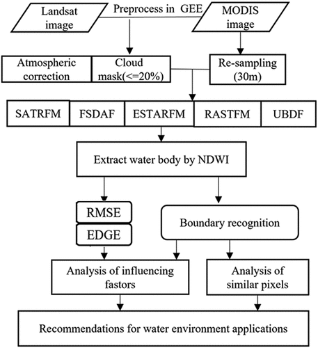
In this research, a comprehensive comparison is made among the following STF algorithms, all of which have been successfully employed in monitoring the water environment: STARFM, ESTARFM, FSDAF, RASTFM, and UBDF. The STF algorithms were applied to a dataset containing 720 images, covering 45 lakes with diverse boundary shapes and varying water quality from around the world. The fusions were then evaluated using both shape and spectral accuracy indices. Furthermore, there are three typical water conditions: water body with complex boundaries, water affected by algae blooms, and water that undergoes seasonal changes. Furthermore, we applied STF to the time series data and analyzed the fusions together with the input multi-source images. At last, recommendations were made for the use of proper algorithm in various water environment monitoring missions. The article also discussed the efficacy and challenges of the current algorithms. The flowchart for this research is depicted in Figure 1.

Figure 1. The flowchart of this research.

2. Data and method

2.1. Study area and data

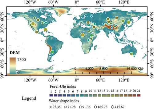
Given the complex nature of inland water systems, the choice of representative water bodies is of paramount importance when evaluating STF algorithms. Ho et al. (2019) selected 71 representative large lakes worldwide to examine the temporal trends of fresh water phytoplankton blooms on a global scale. Accordingly, we selected high-quality Landsat and MODIS data series from the 71 lakes based on the criterion that there are at least 10 clear scenes (cloud coverage is less than 20%) of Landsat images during the study period (year 2021). 45 out of the 71 lakes were selected as study areas for this study (Figure 2). For each of these lakes, we collected Landsat 8 OLI level 2 surface reflectance data and MODIS MOD09GA data from the year 2021. In total, we downloaded 720 images, which comprised 360 quasi-synchronous image pairs for the random experiment. In order to describe the selected water bodies, we calculated their respective Forel-Ule index (FUI) and Water shape index (WSI). FUI was widely used as a simple and effective index to reflect water color. It converts the RGB color index into a color index that each value represents a specific color (Figure 2). WSI is a shape index to represent the complexity of a geometry, using circle as the reference. Furthermore, submersion percentage maps for the water bodies were also generated to illustrate their hydrological characteristics. The detailed steps for generating the character indexes are shown in Appendix B.

Figure 2. Distribution of the 45 lakes and their averaged Forel-Ule index (FUI) and Water shape index (WSI) values. The global DEM data come from GTOPO30 (https://www.usgs.gov/centers/eros/science).

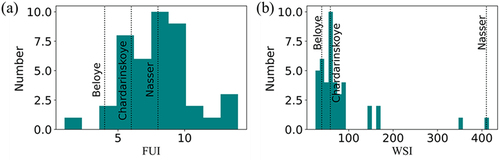
The FUI and WSI indices for the 45 lakes in 2021 were calculated using cloud-free Landsat 8 OLI images. The resulting histograms are depicted in Figure 3. The FUI values are primarily distributed between 6 and 9, representing both clean and eutrophic water conditions. Moreover, the majority of the WSI values fall below 100, indicating that the shapes of the lakes are more regular than intricate.

Figure 3. Histogram of FUI and WSI of the selected lakes.

We selected three representative water bodies to provide a more detailed illustration of the dataset. These include Nasser Lake (Figure 4), which demonstrates complex boundaries; Beloye Lake (Figure 5), which showcases complex water quality; and Chardarinskoye Lake (Figure 6), which represents the rapid changes in water.

Figure 4. False color composited map (a) of Lake Nasser on Sep. 19, 2021, its averaged FUI map (b) and submerge percentage map (c) of year 2021 and typical water surface remote sensing reflectance (Rrs) spectral (d). The red and black lines represent the original Landsat spectral and the atmospheric corrected spectral, respectively. The detailed atmospheric correction method is introduced in section 2.2.1.

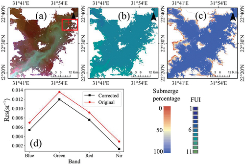
Figure 5. False color composited map (a) of Lake Beloye on Aug. 21, 2021, its averaged FUI map (b) and submerge percentage map (c) of year 2021 and a typical Rrs spectral (d). The red and black lines represent the original Landsat spectral and the atmospheric corrected spectral, respectively. The detailed atmospheric correction method is introduced in section 2.2.1.

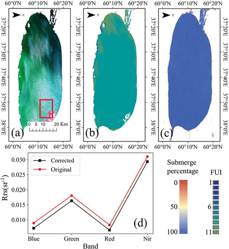
Figure 6. False color composited map (a) of Lake Chardarinskoye on Apr, 16, 2021, its averaged FUI map (b), and submerge percentage map(c) of year 2021, and typical Rrs spectral (d). The red and black lines represent the original Landsat spectral and the atmospheric corrected spectral, respectively. The detailed atmospheric correction method is introduced in section 2.2.1.

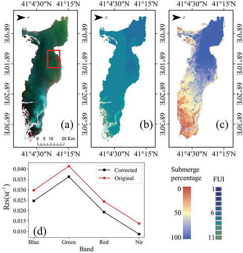
Lake Nasser is a vast reservoir located in southern Egypt and northern Sudan. It covers a total surface area of 5250 km². We focused on the southern section of the reservoir, taking into account its extent and the overall shape of the water body. Lake Beloye, located in the northwestern part of Vologda Oblast in Russia, is one of the largest natural lakes in Europe. The obvious algae blooms Figure 5(a) indicates that the lake is experiencing eutrophication. Lake Chardarinskoye, a reservoir located in southern Kazakhstan. Temporally, the eastern part of the reservoir experiences considerable dynamism Figure 6(c).

2.2. Data processing

2.2.1. Brief introduction to STF algorithms

The five selected STF algorithms can be categorized into three types: the Spatiotemporal weighting algorithms (STARFM, ESTARFM (Zhu et al. 2010), and RASTFM (Zhao, Huang, and Song 2018)); the unmixing-based algorithm (UBDF); and their combined algorithm (FSDAF (Zhu et al. 2016)). In this section, we will first describe the fundamental concepts of the spatiotemporal weighting method and the unmixing-based method. Subsequently, the five STF algorithms will be introduced.

The core hypothesis of the spatiotemporal weighting algorithms is that the land cover types remain unchanged during the prediction interval. Thus, the high-resolution pixel at time t₂ could be estimated using the existing high-resolution pixel at t₁ and the extracted changing information from the low-resolution pixel:

(1) $\begin{array}{c}\mathit{L}\left(\mathit{x},\mathit{y},t_2\right)=\mathit{L}\left(\mathit{x},\mathit{y},t_1\right)+\mathit{M}\left(\mathit{x},\mathit{y},t_2\right)-\mathit{M}\left(\mathit{x},\mathit{y},t_1\right)\end{array}$(1)

The L and M represent pixel reflectance of Landsat and MODIS, respectively; x and y represents the geospatial location of the current pixel.

The unmixing-based method relies on the same assumption as the spatiotemporal weighting method. A typical unmixing process involved decomposing a spectral signal into the abundances of specific endmembers. In unmixing-based strategies, a different approach was used for unmixing: the abundances of different endmembers in a coarse pixel footprint are firstly determined by the high-resolution classification image. The endmembers are then retrieved from the coarse pixel value and abundance array.

STARFM is the base model in spatiotemporal weighting methods. By first selecting similar pixels surrounding the center pixel within a specific window, and then applying the weighted-sum form of Equation (1)(1) $\begin{array}{c}\mathit{L}\left(\mathit{x},\mathit{y},t_2\right)=\mathit{L}\left(\mathit{x},\mathit{y},t_1\right)+\mathit{M}\left(\mathit{x},\mathit{y},t_2\right)-\mathit{M}\left(\mathit{x},\mathit{y},t_1\right)\end{array}$(1) , the center pixel’s value is predicted. The similar pixels were identified based on two criteria: the pixels with a similar difference between Landsat and MOIDS at the base time, and the pixels with a similar changing patterns to the center pixel (Gao et al. 2006b). The ESTARFM algorithm relies on the STARFM algorithm to establish linear relationships between Landsat and MODIS pixels, enhancing the algorithm’s effectiveness in heterogenous regions. The RASTFM algorithm has improved the method of selecting similar pixels. It first searches for non-local similar regions and then selects similar pixels using non-local means. The weightings were further calculated using the locally linear embedding model.

The UBDF algorithm firs retrieves the endmember spectra from the coarse pixels at the target time (t₂) and then assigns them to the corresponding classification maps to complete the fusion. The fusion can be performed once throughout the entire image or using a sliding window. In contrast to the spatiotemporal weighting methods, the final reflectance signal of the UBDF fused image is derived solely from the low-resolution image. Thus, when the high-resolution image cannot provide accurate radiometric information, the UBDF method would yield more reliable results.

The FSDAF algorithm combines the spatiotemporal weighting and unmixing methods. The interesting part is that, instead of directly utilizing the coarse pixels of the input images, the FSDAF algorithm retrieves the changing information using the pixel unmixing method, and then generates the changing item. This process transforms the changing information from MODIS pixels into the unmixed endmembers, resulting in more accurate results.In this study, the STARFM, ESTARFM, UBDF, and FSDAF algorithms were implemented using the IDL 8.5 platform. The RASTFM algorithm was implemented in the ArcGIS platform. The fee parameters utilized in these algorithms are detailed in Table 2. These parameters followed the suggestions of their developers and users (Gao et al. 2006b; Liu et al. 2023; Zhao, Huang, and Song 2018; Zhu et al. 2010; Zhukov et al. 1999).

Table 2. Parameters in the 5 STF algorithms.

Algorithm	Window size (in Landsat pixel scale)	Class number	Similar pixel Number	RRN^a
STARFM	25*25	4	12	–
ESTARFM	25*25	4	20	–
RASTFM	25*25	–	23	0.15
UBDF	17*17	50~100	–	–
FSDAF	20*20	4	20	–

^aRRN: Relative Radiometric Normalization (Y. Du, Teillet, and Cihlar 2002).

2.2.2. Atmospheric correction

In order to limit the influence of complex aerosol, Wang et al. (2016) proposed a simple correction method for MODIS surface reflectance production to make it proper for inland water monitoring:

(2) $\begin{array}{c}{R}_{rs}^C\left(\mathit{i}\right)=\frac{\mathit{R}\left(\mathit{i}\right)-\mathit{min}\left({\mathit{R}}_{\mathit{NIR}}:R_{\mathit{SWIR}}\right)}{\mathit{\pi }}\end{array}$(2)

$R_{rs}^C\left(\mathit{i}\right)$ represents the remote sensing reflectance at the $i^{\mathit{th}}$ band. $\mathit{R}\left(\mathit{i}\right)$ is the surface reflectance of band $\mathit{i}$. $R_{\mathit{NIR}}$and $R_{\mathit{SWIR}}$ represent the surface reflectance value of NIR and SWIR bands, respectively. For MODIS data, 860 and 1240 nm bands were selected as NIR and SWIR bands. For Landsat data, 865 and 1608 nm bands were selected. This method has been successfully used in global scale coastal and inland water researches (Cao, Shen, et al. 2022; Wang et al. 2020).

2.2.3. Accuracy assessment

To effectively compare the performance of the STF algorithms, we need to apply properly accuracy assessment methods on the fusions and reference images. In this study, for each fusion experiment, two Landsat images of a specific water body were firstly picked. Then, one of them were set to be the base image and input into the STF algorithms together with their corresponding MODIS images to generate the fusion. The other Landsat image was regarded as the reference image to assess the performance of the current STF algorithm. Assessing the accuracy of image fusion remains a complex challenge, and researchers have developed numerous indices for this purpose. Examples include Root Mean Square Error (RMSE), Absolute Derivation (AD), Correlation Coefficient (CC), Structural Similarity Index (SSIM) and so on. To comprehensively assess both the spectral and spatial accuracy, we adopt the scheme proposed by Zhu et al. (2022) for evaluating the performance of STF algorithms. The evaluation framework encompasses two indices: RMSE and Robert’s edge (EDGE), as detailed in Table 3. All the RMSE and EDGE values that calculated from each fusion and reference image were illustrated in Taylor diagrams.

Table 3. Equations for calculating metrics.

	Index	Formula	Variables	Range
Spectral accuracy	RMSE	$\mathit{RMSE}=\sqrt{\frac{{\sum }_{i=1}^N{\left(F_i-R_i\right)}^2}{\mathit{N}}}$	Fi: the value of pixel $\mathit{i}$ in the fused image Ri: the value of pixel $\mathit{i}$ in the reference image N: the total number of pixels	[0,1]
Spatial accuracy	EDGE	$\mathrm{Edge}=\left|D_{\mathit{m},\mathit{n}}-D_{\mathit{m}+1,\mathit{n}+1}\right|+$ $\left|D_{\mathit{m},\mathit{n}+1}-D_{\mathit{m}+1,\mathit{n}}\right|$	$D_{\mathit{m},\mathit{n}}$: the value of pixels at $i^{\mathit{th}}$ row and $j^{\mathit{th}}$ column Dm: the value of pixels surrounding the central pixel in a 3 × 3 moving window;	[−1,1]

Furthermore, to investigate the factors influencing fusion performance, we calculated the linear correlations between the Landsat and MODIS images at the base time (R_L-M) and between the MODIS images at the base time and the reference time (R_M-M). R_L-M is used to assess the consistency between Landsat and MODIS images. It will be influenced by systematic differences between sensors, image processing steps, rapid changes in water conditions, and other uncertainties. R_M-M is used to assess the temporal changes during the prediction period.

3. Results

3.1. Overall performances

A total of 950 random experiments were conducted using quasi-synchronous image pairs. Two accuracy indices – RMSE and EDGE – were used to assess the performance of the five STF algorithms. The results were visualized in heatmaps (Figure 7), along with three important features of the dataset: WSI, R_L-M, and R_M-M. R_L-M and R_M-M represent the correlation coefficients between Landsat and MODIS images at the base time, and between MODIS images at the base and target time, respectively. R_L-M is used to measure the consistency of multi-source images. R_M-M quantifies the temporal dynamics throughout the prediction period. Higher R_M-M signify systematic landscape changes during the period, while lower values indicate dramatic changes, such as algae blooms. For each algorithm, the heatmap is organized based on the ascending order of the average R_L-M, and R_M-M values (Figure 7).

Figure 7. Indices heatmaps of ESTARFM (a), FSDAF (b), RASTFM (c), STARFM (d), and UBDF (e).

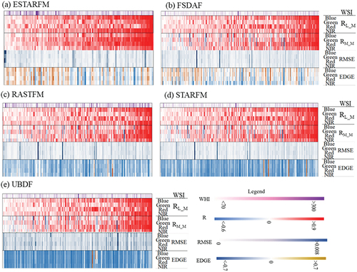
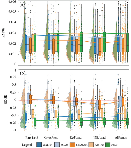
In terms of spectral accuracies, the ESTARFM, FSDAF, RASTFM, and STARFM algorithms exhibit similar performance. Within these four algorithms, ESTARFM shows a slight advantage when both R_L-M, and R_M-M are higher Figure 7(a). This suggests that a higher consistency of input data enhances the performance of ESTARFM. For the remaining three algorithms, higher correlation coefficients do not significantly contribute to performance enhancement. However, lower correlation coefficients always lead to suboptimal results, as indicated by the green parts on the left end of Figure 7(b–d). In comparison, UBDF fusions show poorer performance. This is evident from the visibly green RMSE map in Figure 8(a). In most cases, the indices of UBDF are worse and the boxes are wider, indicating its instability. Furthermore, boxplots (Figure 8) suggest that the ESTARFM and FSDAF algorithms generally outperform the other three algorithms in terms of the RMSE indices. Additionally, when considering the robustness of the algorithms, ESTARFM demonstrates greater stability compared to the FSDAF algorithm. This is evident from the shorter heights of the bars for each specific spectral band.

Figure 8. The RMSE boxplots of STARFM (a), FSDAF (b), ESTARFM (c), RASTFM (d) and UBDF (e), and the EDGE boxplots of STARFM (f), FSDAF (g), ESTARFM (h), RASTFM (i) and UBDF (j).

Spatial accuracy, as evaluated through the EDGE, produces more intricate results compared to spectral accuracy. If we look at EDGE indices, we can categorize these algorithms into two groups: ESTARFM and FSDAF in group #1, and RASTFM, STARFM, and UBDF in group #2. In group #1, the EDGE indices are evenly distributed around 0 and appear lighter in color on the heatmaps, this suggests that these algorithms may randomly lead to slightly over-smoothed or over-sharpened results. For group #2, their heatmaps of EDGE consistently show negative values, indicating that the majority of fusions are over-smoothed.

The spectral and spatial accuracy is unevenly distributed across the four spectral bands (Figure 8). In terms of spectral accuracy, the blue band performs slightly worse than the other bands Figure 8(a). However, this disadvantage is not evident in spatial accuracy Figure 8(b). This may due to the larger uncertainties of the surface reflectance productions in blue band. On the contrary, the NIR band appears to be stable in spectral accuracy Figure 8(a) but it performs worse than the other three bands in spatial accuracy Figure 8(b). The green and red bands are relatively stable across all assessment indexes and spectral bands.

WSI has minimal influence on the performance of STF algorithms in terms of error indices. Further analysis of the specific effects of boundaries will be conducted in section 3.2.1 by a typical dataset.

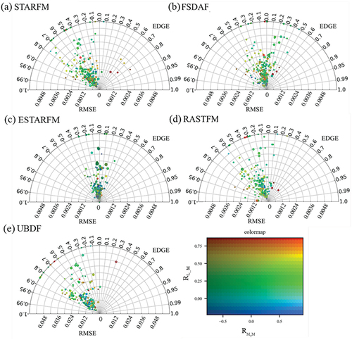
The Taylor diagrams Figures 9–12 introduce another perspective to analyze the overall performance of the five STF algorithms. Utilizing RMSE and EDGE as representations of spectral and spatial accuracies, respectively, a two-dimensional color index of R_M-M and R_L-M was created. The point size corresponds to the amount of WSI value. Overall, the ESTARFM and FSDAF algorithms have similar distributions, scattering evenly around the central vertical line. Comparatively, ESTARFM points tend to be more concentrated along the line compared to FSDAF. Most EDGE values of the ESTARFM algorithm fall within the range of [−0.3, 0.3]. The other three algorithms – STARFM, RASTFM, and UBDF – tend to generate over-smoothed results, with points predominantly located on the left side of the diagram. Moreover, the NIR band is more affected by temporal dynamics than the blue band, resulting in a lower R_M-M for the NIR band. In essence, the NIR band is affected by both sensor preprocessing uncertainties and temporal dynamics, which makes the accurate prediction of the NIR band more challenging compared to other spectral bands.

Figure 9. Taylor diagrams of RMSE and EDGE indices calculated from the blue band of the STARFM (a), FSDAF (b), ESTARFM (c), RASTFM (d), and UBDF (e) fusions.

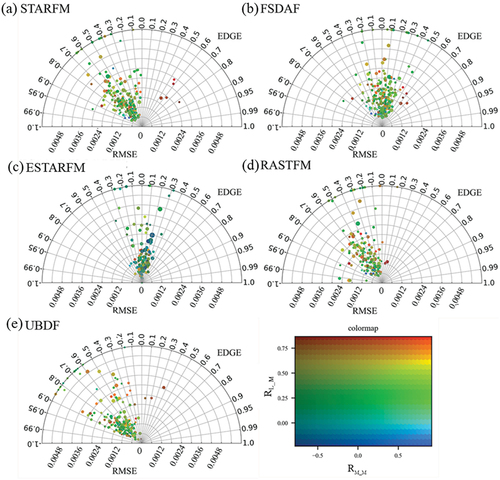
Figure 10. Taylor diagrams of RMSE and EDGE indices calculated from the green band of the STARFM (a), FSDAF (b), ESTARFM (c), RASTFM (d), and UBDF (e) fusions.

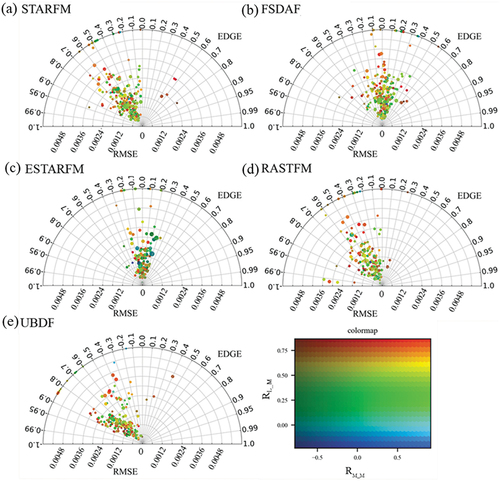
Figure 11. Taylor diagrams of RMSE and EDGE indices calculated from the red band of the STARFM (a), FSDAF (b), ESTARFM (c), RASTFM (d), and UBDF (e) fusions.

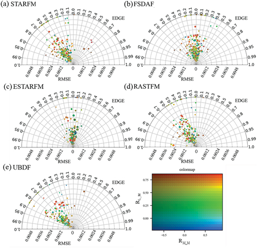
Figure 12. Taylor diagrams of RMSE and EDGE indices calculated from the NIR band of the STARFM (a), FSDAF (b), ESTARFM (c), RASTFM (d), and UBDF (e) fusions.

In addition to the overall distributions, outliers in the Taylor diagram also provide valuable information. A notable example is the presence of dark red dots on the right side of the STARFM diagrams Figure 9(a). These dots correspond to image pairs with low R_M-M and high R_L-M, indicating rapid temporal changes in water bodies in these datasets. In this scenario, FSDAF shows similar performance to STARFM, while ESTARFM and RASTFM are more reliable.

3.2. Performance in typical water bodies

To better demonstrate the fusion performance of the five STF algorithms, we selected three typical image pairs from the complete dataset as introduced in Section 2.1. The color and shape features of these lakes represent three challenging water conditions for STF algorithms: complex boundaries (Lake Nasser), algae blooms (Lake Beloye), and seasonal submersion (Lake Chardarinskoye).

3.2.1. Complex boundary condition

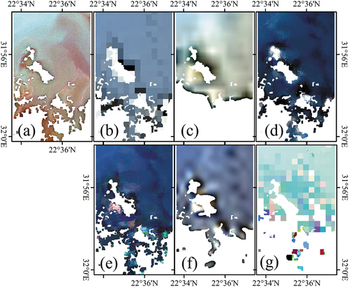
From the map of Lake Nasser Figure A1, a noticeable plume is observed extending from the southwestern to the northeastern side of the lake. In the fusions, the plume is clearly visible in the yields of FSDAF and ESTARFM Figure A1(c,d), and the accuracy is shown in Table 4.

Table 4. Accuracy indices of typical water bodies.

	Nasser		Beloye		Chardarinskoye
	RMSE (sr^−1)	EDGE	RMSE (sr^−1)	EDGE	RMSE (sr^−1)	EDGE
MODIS	3.228×10^−3	−0.628	3.138×10^−3	−0.948	1.093×10^−2	−0.927
STARFM	2.011×10^−3	−0.269	2.979×10^−3	−0.948	1.401×10^−2	−0.644
FSDAF	1.282×10^−3	0.116	2.934×10^−3	−0.765	1.340×10^−2	−0.482
ESTARFM	0.984×10^−3	0.045	2.901×10^−3	−0.726	1.054×10^−2	−0.402
RASTFM	2.404×10^−3	0.107	3.128×10^−3	−0.936	1.313×10^−2	−0.609
UBDF	2.457×10^−3	−0.476	3.128×10^−3	−0.936	1.363×10^−2	−0.559

In Figure 13, we alternatively use the fusions instead of the reference Landsat image to calculate the NDWI indexes and extract water body to test the boundary capture abilities of the algorithms. The results indicate that the FSDAF Figure 13(d) and ESTARFM Figure 13(e) algorithms yield similar results compared to the reference image Figure 13(a). However, some points near the water shore exhibit abnormal colors in the ESTARFM yields, indicating that this algorithm might produce unsatisfactory spectral fidelity in regions with complex water boundaries. The issue arises because highly mixed pixels along the boundary introduce strong error signals during the fusion process. In comparison, FSDAF algorithm effectively addresses this challenge by combining unmixing procedures with the spatiotemporal weighting scheme. The detailed performance of the STFs in this dataset can be found in Figure A4.

Figure 13. Detailed images in the red rectangle marked region in Figure. 3 of Landsat (a), MODIS (b), STARFM (c), FSDAF (d), ESTARFM (e), RASTFM (f), and UBDF (g), respectively.

3.2.2. Algae bloom condition

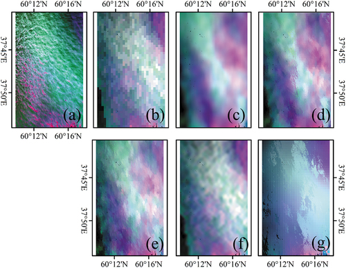
Lake Beloye maintains a stable shape Figure 4 while exhibiting complex water quality. Within the context of the dense algae bloom regions, STARFM Figure A2(b), FSDAF Figure A2(c), and ESTARFM Figure A2(d) effectively capture this area. In contrast, the region appears noticeably blurred in the RASTFM Figure A2(e) and UBDF Figure A2(f) fusions. Shifting the focus to the overall color of the images, the FSDAF and ESTARFM algorithms exhibit superior performance compared to the other three algorithms. This is attributed to their ability of accurately capture the dark green sections in the northern part of the lake.

The algorithms performance varies in local region. A small region encompassing the algae bloom is shown in Figure 14, during bloom, all five STF algorithms show inadequate stability. STARFM Figure 14(c), ESTARFM Figure 14(e), and FSDAF Figure 14(e) algorithms appear to generate more bloom regions compared to the reference Landsat image Figure 14(a). The RASTFM Figure 14(f) and UBDF Figure 14(g) algorithms tend to preserve the actual distribution of the blooms, with RASTFM offering clearer spatial details. However, these two algorithms failed to capture the spatial details of bloom region boundaries.

The accuracy indices of the five STF algorithms (Table 4) indicated that, with the exception of the ESTARFM and FSDAF algorithms, the other three algorithms do not provide better results compared to the original MODIS image. Therefore, in conditions of algae bloom, ESTARFM and FSDAF are recommended. However, due to the overestimation of algae areas by the two algorithms, it is recommended to use original MODIS images for statistical analysis of algae bloom areas. The detailed performance of the STFs in this dataset can be found in Figure A5.

Figure 14. Detailed images in the red rectangle marked region in Figure 4 of Landsat (a), MODIS (b), STARFM (c), FSDAF (d), ESTARFM (e), RASTFM (f), and UBDF (g), respectively.

3.2.3. Seasonal submerge condition

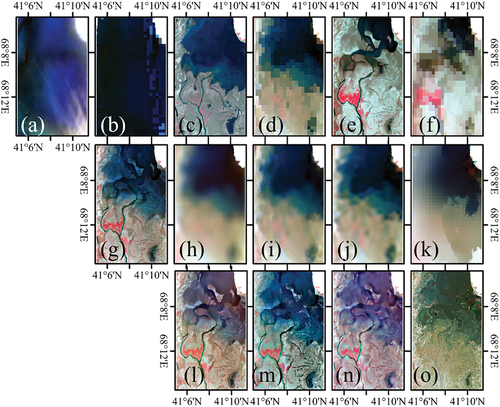
Unlike Lake Beloye, Lake Chardarinskoye exhibits significant temporal dynamism in water levels. The submerge percentage map (Figure 5) reveals spatial variation, making it an ideal case to showcase algorithm performance in similar water bodies undergoing seasonal changes. The results (Figure A3) for 6 August 2021, reveal that only the ESTARFM algorithm produce reasonable fusion: the image has clear textures and proper color. Conversely, the fusions from the STARFM, RASTFM, and UBDF algorithms appear lighter than the reference image. While the FSDAF algorithm produces an image with correct coloring, it is excessively smoothed Figure A3(c), and the accuracy is shown in Table 4. To delve deeper into the factors contributing to this result, we zoomed in on the red-marked region and illustrated two fusion sets that were calculated from the base image pair on 16 April 2021 Figure 15(a) and 17 September 2021 Figure 15(e). The ESTARFM algorithm incorporates both base image pairs, enabling it to successfully trace spatial details from similar pixels. When calculated from the base image pair on 17 September 2021, the other four STF algorithms also retrieve sufficient spatial details Figure 15(l–m). Another conclusion is that when abundant spatial details are used as input, the results tend to be over-sharpened, even for the ESTARFM algorithm. This issue consistently poses a challenge for STF algorithms, as sudden submergence processes contradict the core assumptions of current STFs. This suggests that the base Landsat images often fail to provide sufficient spatial details for the fusion process. Nevertheless, our findings indicate that the current STF algorithms still have the potential to extract submerged regions from fusions when multiple temporal image pairs are employed instead of a single input image pair. The detailed performance of the STFs in this dataset can be found in Figures A6 and A7.

Figure 15. Detailed images in the red rectangle marked region in Figure. 5 of Landsat on Apr. 16, 2021 (a), Aug. 6, 2021(c), Sep. 17, 2021 (e), MODIS on Apr. 16, 2021 (b), Aug. 6, 2021(d), Sep. 17, 2021 (f), and two fusions sets: (g) ~ (k) represents the results of ESTARFM, STARFM, FSDAF, RASTFM, and UBDF that calculated from the base image pair on Apr. 16, 2021, respectively; (l) ~ (o) represents the results of STARFM, FSDAF, RASTFM, and UBDF that calculated from the base image pair on Sep. 17, 2021, respectively. The fusion target date is Aug. 6, 2021. All the detailed scatter plots of the three typical samples could be fund in Figures A4~A7.

3.3. Enhancement of STF to time series analysis

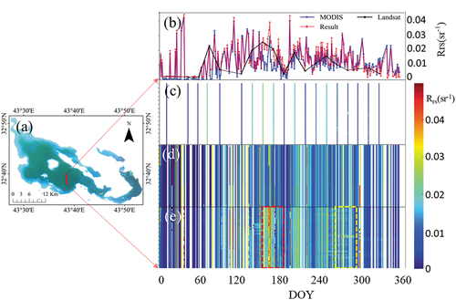
To demonstrate the temporal and spatial effects of integrating STF algorithms in analysis, we employed the top-performing ESTARFM algorithm to generate a complete STF dataset for Lake Razazza in 2021. Subsequently, we extracted a spatial profile from all available Landsat, MODIS, and the fused images, and collectively plotted them in a heatmap.

The results are depicted in Figure 19. To simplify the discussion, only the NIR band is analyzed, as the other bands showed similar patterns. Firstly, the Landsat series exhibits temporal trends that are consistent with those of MODIS. As expected, the MODIS curve captures more intricate temporal trends that were overlooked by Landsat. The ESTARFM fused data adeptly integrates these detailed temporal fluctuations into the Landsat time series Figure 16(e), especially within the region indicated by the red rectangle Figure 16(e). Consequently, the fusions exhibit better alignment with Landsat in terms of value (yellow rectangle Figure 16(e) and successfully capture the detailed temporal fluctuations of MODIS. This could lead to a hidden issue for quantitative water quality monitoring missions: if the high spatial resolution image cannot provide solid surface reflectance production for water images, the resulting fusions will be contaminated. Therefore, quantitative monitoring missions for water environment will require high-accuracy atmospheric correction for high spatial resolution images. If the atmospheric correction accuracy of high spatial resolution images are not guaranteed, which always happens due their lack of useful spectral bands, the UBDF algorithm could provide solid fusions because the radiometric uncertainties of high spatial resolution images would not affect the final fusions.

Figure 16. Temporal changing of a typical profile in Lake Razazza. (a) is a clear image of Lake Razazza in which the red line represents the profile location; (b) is the averaged line chart; (c), (d), and (e) are the temporal heatmap of Landsat, MODIS, and ESTARFM yielded image sets. The unavailable dates that influenced by cloud contamination are left blank in the heatmaps. The red and yellow rectangle-marked regions in this figure are two typical regions to demonstrate the effectiveness of the fusion results.

3.4. Recommendations for selecting STF algorithms

Considering all the above analysis, we are able to offer specific recommendations for the implement of STF algorithms in different water environment monitoring missions. The results are summarized in Table 5.

Table 5. Ranking of STF algorithms in water environment monitoring.

	STARFM	ESTARFM	FSDAF	RASTFM	UBDF
Water body extraction	4	1	2	3	5
Algae bloom detection	5	1	2	3	4
Seasonal water body monitoring	4	1	2	3	5
Quantitative monitoring	5	1	2	4	3

Water body extraction is crucial for detecting the storage of fresh water (Topp et al. 2020) and its long-term trends. Our experiment on Lake Nasser demonstrated that both the ESTARFM and FSDAF algorithms can effectively provide accurate water boundary information using a simple threshold extraction method (Figure 13). For algae bloom detection missions, all current algorithms face challenges, but the ESTARFM and FSDAF algorithms tend to yield relatively better results. For seasonal water body monitoring, the most significant challenge is that the change in water submergence can lead to temporal dynamic in land cover types. Nevertheless, the ESTARFM algorithm outperformed the other four algorithms and yielded reasonable results. This implies that spatial information can still be retrieved even for cyclically changing water bodies, where land cover changes during the prediction period. The ESTARFM algorithm faces the challenge of tending to produce over-sharpened results under these conditions. If the mission primarily focuses on seasonal water body coverage, ESTARFM could be a suitable choice. For quantitative monitoring missions, among the three recommended algorithms, ESTARFM and FSDAF algorithms are preferable because they exhibit lower uncertainties in spectral accuracy indices. UBDF is also a viable choice, particularly if the high temporal resolution dataset has better atmospheric correction accuracy than the high spatial resolution dataset. UBDF’s advantage lies in its ability to maintain spectral fidelity in the fusion. This advantage has been demonstrated in previous research. However, the spatial accuracy of UBDF is unsatisfactory in this study. Hence, refining the UBDF algorithm to improve its spatial accuracy is a potential area for future research.

4. Discussion

4.1. Challenges for STF algorithms in inland water monitoring

The overall performance of the STFs Figure 18 indicates that generating accurate fusions of the blue and NIR bands is more challenging than fusing the other bands. The colors of the points in Taylor diagrams Figures 9–12 reveal that the blue and NIR bands produce greener points compared to the green and red bands. Simultaneously, NIR band points appear darker than those in the blue band. This suggests that the consistency between Landsat and MODIS is lower in the blue and NIR bands compared to the green and red bands. Considering this analysis alongside Figure 8, it can be inferred that this inconsistency is the primary factor influencing the fusion accuracy.

For the blue band, this inconsistency might be due to atmospheric correction. H. Liu et al. (2022) and Pahlevan et al. (2021)tested several widely used atmospheric correction methods using large datasets collected from inland global lakes and rivers (Liu et al. 2021; Pahlevan et al. 2021). They concluded that the uncertainty of the blue band is larger than that of the other bands. This results in greater inconsistency between Landsat and MODIS images in the blue band.

The inconsistency of the NIR band is attributed to the rapidly changing algae conditions. Li et al. (2022b) found that the upward floating speed of cyanobacteria in Taihu Lake can be up to nearly 0.9 m/h. This will lead to obvious spatial distribution variations even within an hour’s temporal window (Guo et al. 2020; Li et al. 2022b). Compared with the other bands, the radiative signal in the NIR band is more sensitive to algae (Hu 2009). Therefore, the time lag between Landsat and MODIS acquisitions results in horizontal and vertical displacement of algae, further influencing the consistency of their NIR images. This divergence directly affects the performance of STF algorithms.

4.2. Uncertainty sources of different STF strategies

Uncertainties in the algorithms are primarily focused on two basics of the five STF algorithms: spatiotemporal weighting and pixel unmixing. The two strategies correspond to STARFM-like and UBDF algorithms, respectively. STARFM-like algorithms share the theoretical basis that STF fusion involves injecting changing information into the base high-resolution image (Formula 1). The primary source of information for fusion is high-resolution images. Thus, two fundamental steps of STARFM-like algorithms involve searching for similar pixels and capturing changing information from low-resolution images, with the aim of enhancing the accuracy of the injected information. The previous researches do not address the uncertainty associated with high-resolution images, such as Landsat images, in the STARFM algorithm. It is reasonable to fuse Landsat and MODIS images of terrestrial targets because the radiometric consistency of these two data sources has been widely discussed. Under these conditions, the Landsat image can be considered the “ground truth” and serves as the foundation for the fusion algorithm. However, when using other image data or when facing a waterbody, the accuracy of the “ground truth” is questionable. For other multisource data, differences in spectral reflectance, orbiting height, FOV settings, will all influence their consistency. For water imagery, normal atmospheric correction can lead to significant variations among different sensors. If high-resolution images contain more reliable radiometric information, the theoretical foundation remains valid. However, when low-resolution images have fewer uncertainties, which is more common for water color sensors such as MERIS and Sentinel-3 OLCI, which data source is closer to the “ground truth” remains an issue for discussion. Thus, STARFM-like algorithms are more sensitive to the radiometric consistency of input multisource images. Even though the FSDAF algorithm combines spatiotemporal weighting and unmixing processes, the unmixing process serves as an agent to capture changing information more accurately. Therefore, it is also classified as STARFM-like algorithms.

The UBDF algorithm integrates multi-source information using an alternative strategy. It unmixes the low-resolution pixels and reassign endmember values to the high-resolution class image. The result of this algorithm is constrained by the low-resolution pixels, in another word, the basic information. Thus, the UBDF algorithm relies more on the radiometric information of the low-resolution image than on the high-resolution image. This hypothesis perfectly overcomes the problem that STARFM-like algorithms face. Guo’s study (Guo et al. 2015) supports the effectiveness of UBDF for quantitatively monitoring of water environments. However, the uncertainties of the UBDF algorithm mainly arise from the spatial aspect: the unmixing process involves percentages of endmembers that are calculated from high-resolution images. The uncertainties of this algorithm will increase under the following two conditions: frequent temporal changes in the water surface or insufficient accuracy in the georeferencing process.

In conclusion, the STARFM-like and UBDF algorithms have different uncertainty sources. This requires careful consideration before applying them in water environment monitoring missions.

4.3. Shortcomings and outlooks

The quality of input data is always important for image fusion algorithms. In this study, we employed a simple correction to MODIS and Landsat land surface reflectance production to control the atmospheric correction errors. Although this method has been reported as effective for both inland and coastal waters in previous studies, its uncertainty was not thoroughly discussed. As water-leaving radiance is always weak compared to other targets, it poses serious challenges for atmospheric correction. Furthermore, inland water upwelling radiance signals can be badly influenced by complex particulate emissions in the air resulting from surrounding human activities. Accurate atmospheric correction of inland water images remains an unresolved problem. With accurate atmospheric correction, the findings and discussions of this study will be more convincing.

This study revealed that water imagery is distinct from terrestrial imagery in STF missions. Fully utilizing temporal trend information is essential for water image STF algorithms because the assumption of similar pixels is facing strong challenges. Previous studies (Guo et al. 2020, 2021) indicate that the temporal unmixing method can successfully retrieve changes in water surface reflectance from time series images, even when water conditions change frequently. Even though its effectiveness has not been tested in long-term image sets, temporal unmixing is a potential technique for inland water STF algorithms. In addition, deep learning methods are receiving widespread attention in STF algorithms due to their strong end-to-end fitting ability (Liu et al. 2016; Wang et al. 2022). By carefully considering the error distribution in multi-source water images, deep learning methods will provide powerful assistant for STF algorithms for water images.

5. Conclusions

We carried out a comprehensive comparison of five STF algorithms in fresh water remote sensing missions. The following conclusions are drawn.

1. Overall, ESTARFM algorithm outperforms the other four algorithms in both visual effect and accuracy indices assessment.

2. ESTARFM and FSDAF algorithms are recommended in water body extraction; FSDAF algorithm is recommended in algae bloom detection; ESTARFM, FSDAF, and UBDF algorithms are recommended in quantitative monitoring; ESTARFM algorithm is recommended in seasonal water body monitoring.

3. STARFM-like algorithms are sensitive to radiometric uncertainties and UBDF algorithm is sensitive to spatial uncertainties.

4. Rapidly changing water conditions, such as algae blooms, continue to pose a significant challenge for the five famous STF algorithms. More effort should be devoted to this problem in future research.

Acknowledgment

The authors wish to thank Professor Xiaolin Zhu for sharing the code of STARFM, ESTARFM and FSDAF algorithms. We also wish to acknowledge Professor Yongquan Zhao for sharing the toolbox of RASTFM algorithm.

Disclosure statement

The authors declare that they have no known competing financial interests or personal relationships that could have appeared to influence the work reported in this paper.

Data availability statement

Data will be made available on request.

Additional information

Funding

The work was supported by the National Natural Science Foundation of China [grant number 41701422]; National Natural Science Foundation of China [grant number 42071333]; National Key R & D Program of China [grant number 2021YFD1700900].

Appendix A

Figure A1. The false color composited (R: NIR band; G: red band; B: green band) image of reference Landsat (a), STARFM (b), FSDAF (c) ESTARFM (d), RASTFM (e), and UBDF (f) fusions of Lake Nasser on Sep. 19, 2021.

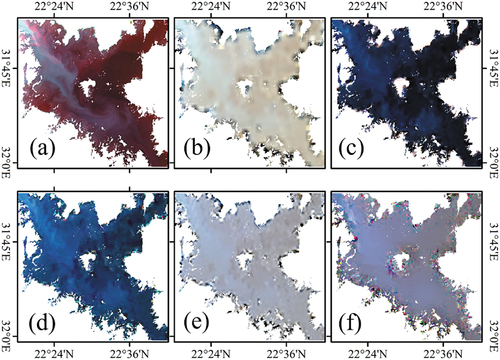
Figure A2. The false color composited (R: NIR band; G: red band; B: green band) image of reference Landsat (a), STARFM (b), FSDAF (c), ESTARFM (d), RASTFM (e), and UBDF (f) yields of Lake Beloye on Aug. 21, 2021.

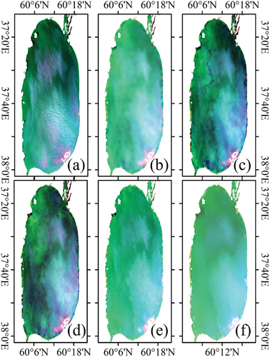
Figure A3. The false color composited (R: NIR band; G: red band; B: green band) image of reference Landsat (a), STARFM (b), FSDAF (c), ESTARFM (d), RASTFM (e), and UBDF (f) yields of Lake Chardarinskoye on Aug. 6, 2021.

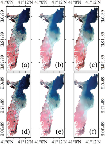
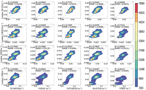
Figure A4. Scatter plots of the fusions from five STFs and the reference image of Lake Beloye.

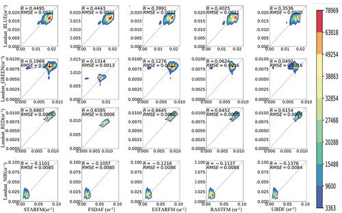
Figure A5. Scatter plots of the fusions from five STFs and the reference image of Lake Nasser.

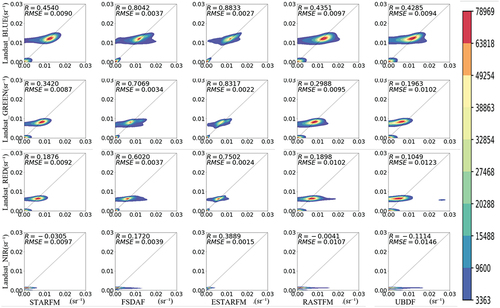
Figure A6. Scatter plots of the fusions from five STFs and the reference image of Lake Chardarinskoye.

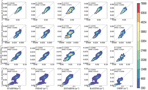
Figure A7. Scatter plots of the fusions from five STFs and the reference image of Lake Chardarinskoye.

Appendix B

FUI, WSI, and submerge percentage were used to describe the characters of the waterbodies.

The FUI was used to describe the color of water. It is calculated by the following equations and Table B1:

(B1) $\begin{array}{c}\mathit{X}=2.7689\mathit{R}+1.7517\mathit{G}+1.1302\mathit{B}\end{array}$(B1)

(B2) $\begin{array}{c}\mathit{Y}=1.00\mathit{R}+4.5907\mathit{G}+0.0601\mathit{B}\end{array}$(B2)

(B3) $\begin{array}{c}\mathit{Z}=0.00\mathit{R}+0.0565\mathit{G}+5.5943\mathit{B}\end{array}$(B3)

(B4) $\begin{array}{c}\begin{array}{c}\mathit{x}=\frac{X}{\mathit{X}+\mathit{Y}+\mathit{Z}}\\ \mathit{\hspace{0.17em}}\end{array}\end{array}$(B4)

(B5) $\begin{array}{c}\mathit{y}=\frac{Y}{\mathit{X}+\mathit{Y}+\mathit{Z}}\end{array}$(B5)

(B6) $\begin{array}{c}\left.\mathit{\alpha }=\left(arctan\left(\mathit{y}\right.,-\frac{1}{3}\mathit{x}-\frac{1}{3}\right)\mathit{\hspace{0.17em}}\mathit{modulus}\mathit{\hspace{0.17em}}2\mathit{\pi }\right)\times 180/\mathit{\pi }\end{array}$(B6)

The R, G, and B represent reflectance of blue, green, and red band, respectively. After α was calculated, the FUI value is then decided from Table B1.

Table B1. Corresponding hue angle α of FUI indices from 1 to 21.

FUI	α	FUI	α	FUI	α
1	229.533	8	99.5371	15	47.8847
2	224.8037	9	88.5017	16	42.3707
3	217.1473	10	78.1648	17	37.1698
4	202.8305	11	70.9617	18	32.6477
5	178.702	12	64.9378	19	28.2408
6	147.4148	13	59.4234	20	24.4487
7	118.5208	14	53.4431	21	21.0471

where R, G, and B represents the reflectance of red, green, and blue bands, respectively.

The WSI represents the shape complexity of the lake. A larger WSI means a more complex shape of the water body. It is calculated by:

(B7) $\begin{array}{c}\mathit{WSI}=\mathit{A}\ast \frac{C^2}{\mathit{S}}\end{array}$(B7)

where A is a constant that used to adjust the scale of WSI. In this research, A is set to 1. C and S represents the perimeter and area of s specific lake.

The submerge percentage to represent the amount of submerge change within a year, it was extracted from JRC dataset in Google Earth Engine (Pekel et al. 2016). This dataset contains maps of the location and temporal distribution of surface water from 1984 to 2022 and provides statistics on the extent and change of those water surfaces that generated from millions of Landsat images.

References

- Cao, Z., R. Ma, N. Pahlevan, M. Liu, J. M. Melack, H. Duan, K. Xue, and M. Shen. 2022. “Evaluating and Optimizing VIIRS Retrievals of Chlorophyll-A and Suspended Particulate Matter in Turbid Lakes Using a Machine Learning Approach.” IEEE Transactions on Geoscience and Remote Sensing 60: 1–30. https://doi.org/10.1109/TGRS.2022.3220529.
- Cao, Z., M. Shen, T. Kutser, M. Liu, T. Qi, J. Ma, R. Ma, and H. Duan. 2022. “What Water Color Parameters Could Be Mapped Using MODIS Land Reflectance Products: A Global Evaluation Over Coastal and Inland Waters.” Earth Science Review 232: 104154. https://doi.org/10.1016/j.earscirev.2022.104154.
- Chang, N. B., K. Bai, and C. F. Chen. 2017. “Integrating Multisensor Satellite Data Merging and Image Reconstruction in Support of Machine Learning for Better Water Quality Management.” Journal of Environmental Management 201: 227–240. https://doi.org/10.1016/j.jenvman.2017.06.045.
- Chang, N.-B., B. W. Vannah, Y. J. Yang, and M. Elovitz. 2014. “Integrated Data Fusion and Mining Techniques for Monitoring Total Organic Carbon Concentrations in a Lake.” International Journal of Remote Sensing 35 (3): 1064–1093. https://doi.org/10.1080/01431161.2013.875632.
- Chen, B., L. Chen, B. Huang, R. Michishita, and B. Xu. 2018. “Dynamic Monitoring of the Poyang Lake Wetland by Integrating Landsat and MODIS Observations.” ISPRS Journal of Photogrammetry and Remote Sensing 139: 75–87. https://doi.org/10.1016/j.isprsjprs.2018.02.021.
- Chen, X., S. Shang, Z. Lee, L. Qi, J. Yan, and Y. Li. 2019. “High-Frequency Observation of Floating Algae from AHI on Himawari-8.” Remote Sensing of Environment 227: 151–161. https://doi.org/10.1016/j.rse.2019.03.038.
- Cui, J., Y. Guo, Q. Xu, D. Li, W. Chen, L. Shi, G. Ji, and L. Li. 2023. “Extraction of Information on the Flooding Extent of Agricultural Land in Henan Province Based on Multi-Source Remote Sensing Images and Google Earth Engine.” Agronomy 13 (2): 355. https://doi.org/10.3390/agronomy13020355.
- Dai, Y., S. Yang, D. Zhao, C. Hu, W. Xu, D. M. Anderson, Y. Li, et al. 2023. “Coastal Phytoplankton Blooms Expand and Intensify in the 21st Century.” Nature 615 (7951): 280–284. https://doi.org/10.1038/s41586-023-05760-y.
- Doña, C., N. B. Chang, V. Caselles, J. M. Sánchez, A. Camacho, J. Delegido, and B. W. Vannah. 2015. “Integrated Satellite Data Fusion and Mining for Monitoring Lake Water Quality Status of the Albufera de Valencia in Spain.” Journal of Environmental Management 151: 416–426. https://doi.org/10.1016/j.jenvman.2014.12.003.
- Duan, P., F. Zhang, C.-Y. Jim, M. L. Tan, Y. Cai, J. Shi, C. Liu, W. Wang, and Z. Wang. 2023. “Reconstruction of Sentinel Images for Suspended Particulate Matter Monitoring in Arid Regions.” Remote Sensing 15 (4): 872. https://doi.org/10.3390/rs15040872.
- Du, Y., P. M. Teillet, and J. Cihlar. 2002. “Radiometric Normalization of Multitemporal High-Resolution Satellite Images with Quality Control for Land Cover Change Detection.” Remote Sensing of Environment 82 (1): 123–134. https://doi.org/10.1016/S0034-4257(02)00029-9.
- Du, C., Q. Wang, Y. Li, H. Lyu, L. Zhu, Z. Zheng, S. Wen, G. Liu, and Y. Guo. 2018. “Estimation of Total Phosphorus Concentration Using a Water Classification Method in Inland Water.” International Journal of Applied Earth Observation and Geoinformation 71: 29–42. https://doi.org/10.1016/j.jag.2018.05.007.
- Feng, L., Y. Dai, X. Hou, Y. Xu, J. Liu, and C. Zheng. 2021. “Concerns About Phytoplankton Bloom Trends in Global Lakes.” Nature 590 (7846): E35–E47. https://doi.org/10.1038/s41586-021-03254-3.
- Gao, F., J. Masek, M. Schwaller, and F. Hall. 2006b. “On the Blending of the Landsat and MODIS Surface Reflectance: Predicting Daily Landsat Surface Reflectance.” IEEE Transactions on Geoscience and Remote Sensing 44 (8): 2207–2218. https://doi.org/10.1109/TGRS.2006.872081.
- Guo, Y., W. Chen, X. Feng, Y. Zhang, Y. Li, C. Huang, and Y. Li. 2021. “Temporal Unmixing-Based Cloud Removal Algorithm for Optically Complex Water Images.” International Journal of Remote Sensing 42 (12): 4415–4440. https://doi.org/10.1080/01431161.2021.1892853.
- Guo, Y., C. Huang, Y. Zhang, Y. Li, and W. Chen. 2020. “A Novel Multitemporal Image-Fusion Algorithm: Method and Application to GOCI and Himawari Images for Inland Water Remote Sensing.” IEEE Transactions on Geoscience and Remote Sensing 58 (6): 4018–4032. https://doi.org/10.1109/TGRS.2019.2960322.
- Guo, Y., Y. Li, L. Zhu, G. Liu, S. Wang, and C. Du. 2015. “An Improved Unmixing-Based Fusion Method: Potential Application to Remote Monitoring of Inland Waters.” Remote Sensing 7 (2): 1640–1666. https://doi.org/10.3390/rs70201640.
- Ho, J. C., A. M. Michalak, and N. Pahlevan. 2019. “Widespread Global Increase in Intense Lake Phytoplankton Blooms Since the 1980s.” Nature 574 (7780): 667–670. https://doi.org/10.1038/s41586-019-1648-7.
- Hu, C. 2009. “A Novel Ocean Color Index to Detect Floating Algae in the Global Oceans.” Remote Sensing of Environment 113 (10): 2118–2129. https://doi.org/10.1016/j.rse.2009.05.012.
- Huang, C., Y. Chen, S. Zhang, L. Li, K. Shi, and R. Liu. 2016. “Surface Water Mapping from Suomi NPP-VIIRS Imagery at 30 M Resolution via Blending with Landsat Data.” Remote Sensing 8 (8): 631. https://doi.org/10.3390/rs8080631.
- Huang, C., K. Shi, H. Yang, Y. Li, A. X. Zhu, D. Sun, L. Xu, et al. 2015. “Satellite Observation of Hourly Dynamic Characteristics of Algae with Geostationary Ocean Color Imager (GOCI) Data in Lake Taihu.” Remote Sensing of Environment 159: 278–287. https://doi.org/10.1016/j.rse.2014.12.016.
- Imen, S., N.-B. Chang, and Y. J. Yang. 2015. “Developing the Remote Sensing-Based Early Warning System for Monitoring TSS Concentrations in Lake Mead.” Journal of Environmental Management 160: 73–89. https://doi.org/10.1016/j.jenvman.2015.06.003.
- Kutser, T. 2012. “The Possibility of Using the Landsat Image Archive for Monitoring Long Time Trends in Coloured Dissolved Organic Matter Concentration in Lake Waters.” Remote Sensing of Environment 123: 334–338. https://doi.org/10.1016/j.rse.2012.04.004.
- Lee, Z., C. Hu, R. Arnone, and Z. Liu. 2012. “Impact of Sub-Pixel Variations on Ocean Color Remote Sensing Products.” Optics Express 20 (19): 20844. https://doi.org/10.1364/OE.20.020844.
- Le, C., Y. Li, Y. Zha, D. Sun, C. Huang, and H. Lu. 2009. “A Four-Band Semi-Analytical Model for Estimating Chlorophyll a in Highly Turbid Lakes: The Case of Taihu Lake, China.” Remote Sensing of Environment 113 (6): 1175–1182. https://doi.org/10.1016/j.rse.2009.02.005.
- Li, J., M. Ke, Y. Ma, and J. Cui. 2022a. “Remote Monitoring of NH3-N Content in Small-Sized Inland Waterbody Based on Low and Medium Resolution Multi-Source Remote Sensing Image Fusion.” Water 14 (20): 3287. https://doi.org/10.3390/w14203287.
- Li, P., Y. Ke, D. Wang, H. Ji, S. Chen, M. Chen, M. Lyu, and D. Zhou. 2021. “Human Impact on Suspended Particulate Matter in the Yellow River Estuary, China: Evidence from Remote Sensing Data Fusion Using an Improved Spatiotemporal Fusion Method.” Science of the Total Environment 750: 141612. https://doi.org/10.1016/j.scitotenv.2020.141612.
- Li, J., Y. Li, S. Bi, J. Xu, F. Guo, H. Lyu, X. Dong, and X. Cai. 2022b. “Utilization of GOCI Data to Evaluate the Diurnal Vertical Migration of Microcystis aeruginosa and the Underlying Driving Factors.” Journal of Environmental Management 310: 114734. https://doi.org/10.1016/j.jenvman.2022.114734.
- Li, X., F. Ling, G. M. Foody, Y. Ge, Y. Zhang, and Y. Du. 2017. “Generating a Series of Fine Spatial and Temporal Resolution Land Cover Maps by Fusing Coarse Spatial Resolution Remotely Sensed Images and Fine Spatial Resolution Land Cover Maps.” Remote Sensing of Environment 196: 293–311. https://doi.org/10.1016/j.rse.2017.05.011.
- Liu, X., C. Deng, S. Wang, G.-B. Huang, B. Zhao, and P. Lauren. 2016. “Fast and Accurate Spatiotemporal Fusion Based Upon Extreme Learning Machine.” Geoscience and Remote Sensing Letters, IEEE 13 (12): 2039–2043. https://doi.org/10.1109/LGRS.2016.2622726.
- Liu, H., X. He, Q. Li, X. Hu, J. Ishizaka, S. Kratzer, C. Yang, et al. 2021. “Evaluation of Ocean Color Atmoshperic Correction Methods for Sentinel-3 OLCI Using Global Automatic in-Situ Observations.” IEEE Transactions on Geoscience & Remote Sensing 60: 1–19. https://doi.org/10.1109/TGRS.2021.3136243.
- Liu, H., X. He, Q. Li, X. Hu, J. Ishizaka, S. Kratzer, C. Yang, et al. 2022. “Evaluation of Ocean Color Atmospheric Correction Methods for Sentinel-3 OLCI Using Global Automatic in situ Observations.” IEEE Transactions on Geoscience and Remote Sensing 60: 1–19. https://doi.org/10.1109/TGRS.2021.3136243.
- Liu, G., S. G. H. Simis, L. Li, Q. Wang, Y. Li, K. Song, H. Lyu, et al. 2018. “A Four-Band Semi-Analytical Model for Estimating Phycocyanin in Inland Waters from Simulated MERIS and OLCI Data.” IEEE Transactions on Geoscience and Remote Sensing 56 (3): 1374–1385. https://doi.org/10.1109/TGRS.2017.2761996.
- Liu, C., F. Zhang, M. L. Tan, C.-Y. Jim, K. Song, J. Shi, X. Lin, et al. 2023. “High Spatiotemporal Resolution Reconstruction of Suspended Particulate Matter Concentration in Arid Brackish Lake, China.” Journal of Cleaner Production 414: 137673. https://doi.org/10.1016/j.jclepro.2023.137673.
- Li, N., Y. Zhang, K. Shi, Y. Zhang, X. Sun, W. Wang, H. Qian, H. Yang, and Y. Niu. 2023. “Real-Time and Continuous Tracking of Total Phosphorus Using a Ground-Based Hyperspectral Proximal Sensing System.” Remote Sensing 15 (2): 507. https://doi.org/10.3390/rs15020507.
- Mangiarotti, S., J.-M. Martinez, M.-P. Bonnet, D. C. Buarque, N. Filizola, and P. Mazzega. 2013. “Discharge and Suspended Sediment Flux Estimated Along the Mainstream of the Amazon and the Madeira Rivers (From in situ and MODIS Satellite Data).” International Journal of Applied Earth Observation and Geoinformation 21: 341–355. https://doi.org/10.1016/j.jag.2012.07.015.
- Meng, Q., J. Song, Y. Fu, Y. Cai, J. Guo, M. Liu, and X. Jiang. 2023. “Downscaling of Oceanic Chlorophyll-A with a Spatiotemporal Fusion Model: A Case Study on the North Coast of the Yellow Sea.” Water 15 (20): 3566. https://doi.org/10.3390/w15203566.
- Minghelli-Roman, A., L. Polidori, S. Mathieu-Blanc, L. Loubersac, and F. Cauneau. 2007. “Fusion of MeRIS and ETM Images for Coastal Water Monitoring.” IEEE International Geoscience and Remote Sensing Symposium, 2007, Barcelona, Spain. 322–325. https://doi.org/10.1109/IGARSS.2007.4422795.
- Moosavi, V., A. Talebi, M. H. Mokhtari, S. R. F. Shamsi, and Y. Niazi. 2015. “A Wavelet-Artificial Intelligence Fusion Approach (WAIFA) for Blending Landsat and MODIS Surface Temperature.” Remote Sensing of Environment 169: 243–254. https://doi.org/10.1016/j.rse.2015.08.015.
- Oyama, Y., T. Fukushima, B. Matsushita, H. Matsuzaki, K. Kamiya, and H. Kobinata. 2015. “Monitoring Levels of Cyanobacterial Blooms Using the Visual Cyanobacteria Index (VCI) and Floating Algae Index (FAI).” International Journal of Applied Earth Observation and Geoinformation 38: 335–348. https://doi.org/10.1016/j.jag.2015.02.002.
- Pahlevan, N., A. Mangin, S. V. Balasubramanian, B. Smith, K. Alikas, K. Arai, C. Barbosa, et al. 2021. “ACIX-Aqua: A Global Assessment of Atmospheric Correction Methods for Landsat-8 and Sentinel-2 Over Lakes, Rivers, and Coastal Waters.” Remote Sensing of Environment 258: 112366. https://doi.org/10.1016/j.rse.2021.112366.
- Pahlevan, N., B. Smith, K. Alikas, J. Anstee, C. Barbosa, C. Binding, M. Bresciani, et al. 2022. “Simultaneous Retrieval of Selected Optical Water Quality Indicators from Landsat-8, Sentinel-2, and Sentinel-3. Remote Sens.” Remote Sensing of Environment 270: 112860. https://doi.org/10.1016/j.rse.2021.112860.
- Pekel, J.-F., A. Cottam, N. Gorelick, and A. S. Belward. 2016. “High-Resolution Mapping of Global Surface Water and Its Long-Term Changes.” Nature 540 (7633): 418–422. https://doi.org/10.1038/nature20584.
- Ruddick, K. G., H. J. Gons, M. Rijkeboer, and G. Tilstone. 2001. “Optical Remote Sensing of Chlorophyll a in Case 2 Waters by Use of an Adaptive Two-Band Algorithm with Optimal Error Properties.” Applied Optics 40 (21): 3575. https://doi.org/10.1364/ao.40.003575.
- Sahoo, D. P., B. Sahoo, and M. K. Tiwari. 2022a. “MODIS-Landsat Fusion-Based Single-Band Algorithms for TSS and Turbidity Estimation in an Urban-Waste-Dominated River Reach.” Water Research 224: 119082. https://doi.org/10.1016/j.watres.2022.119082.
- Sahoo, D. P., B. Sahoo, and M. K. Tiwari. 2022b. “MODIS-Landsat Fusion-Based Single-Band Algorithms for TSS and Turbidity Estimation in an Urban-Waste-Dominated River Reach.” Water Research 224: 119082. https://doi.org/10.1016/j.watres.2022.119082.
- Shenglei, W., L. Junsheng, Z. Bing, S. Qian, Z. Fangfang, and L. Zhaoyi. 2016. “A Simple Correction Method for the MODIS Surface Reflectance Product Over Typical Inland Waters in China.” International Journal of Remote Sensing 37 (24): 6076–6096. https://doi.org/10.1080/01431161.2016.1256508.
- Sherman, J., M. Tzortziou, K. J. Turner, J. Goes, and B. Grunert. 2023. “Chlorophyll Dynamics from Sentinel-3 Using an Optimized Algorithm for Enhanced Ecological Monitoring in Complex Urban Estuarine Waters.” International Journal of Applied Earth Observation and Geoinformation 118: 103223. https://doi.org/10.1016/j.jag.2023.103223.
- Shi, K., Y. Zhang, G. Zhu, X. Liu, Y. Zhou, H. Xu, B. Qin, et al. 2015. “Long-Term Remote Monitoring of Total Suspended Matter Concentration in Lake Taihu Using 250m MODIS-Aqua Data.” Remote Sensing of Environment 164: 43–56. https://doi.org/10.1016/j.rse.2015.02.029.
- Sun, D., C. Hu, Z. Qiu, J. P. Cannizzaro, and B. B. Barnes. 2014. “Influence of a Red Band-Based Water Classification Approach on Chlorophyll Algorithms for Optically Complex Estuaries.” Remote Sensing of Environment 155: 289–302. https://doi.org/10.1016/j.rse.2014.08.035.
- Swain, R., and B. Sahoo. 2017. “Mapping of Heavy Metal Pollution in River Water at Daily Time-Scale Using Spatio-Temporal Fusion of MODIS-Aqua and Landsat Satellite Imageries.” Journal of Environmental Management 192: 1–14. https://doi.org/10.1016/j.jenvman.2017.01.034.
- Topp, S. N., T. M. Pavelsky, D. Jensen, M. Simard, and M. R. V. Ross. 2020. “Research Trends in the Use of Remote Sensing for Inland Water Quality Science: Moving Towards Multidisciplinary Applications.” Water 12 (1): 169. https://doi.org/10.3390/w12010169.
- Topp, S. N., T. M. Pavelsky, E. H. Stanley, X. Yang, C. G. Griffin, and M. R. V. Ross. 2021. “Multi-Decadal Improvement in US Lake Water Clarity.” Environmental Research Letters 16 (5): 055025. https://doi.org/10.1088/1748-9326/abf002.
- Vanhellemont, Q., G. Neukermans, and K. Ruddick. 2014. “Synergy Between Polar-Orbiting and Geostationary Sensors: Remote Sensing of the Ocean at High Spatial and High Temporal Resolution.” Remote Sensing of Environment 146: 49–62. https://doi.org/10.1016/j.rse.2013.03.035.
- Wang, Q., X. Ding, X. Tong, and P. M. Atkinson. 2022. “Real-Time Spatiotemporal Spectral Unmixing of MODIS Images.” IEEE Transactions on Geoscience and Remote Sensing 60: 1–16. https://doi.org/10.1109/TGRS.2021.3108540.
- Wang, S., J. Li, B. Zhang, Z. Lee, E. Spyrakos, L. Feng, C. Liu, et al. 2020. “Changes of Water Clarity in Large Lakes and Reservoirs Across China Observed from Long-Term MODIS. Remote Sens.” Remote Sensing of Environment 247: 111949. https://doi.org/10.1016/j.rse.2020.111949.
- Wang, S., J. Li, B. Zhang, Q. Shen, F. Zhang, and Z. Lu. 2016. “A Simple Correction Method for the MODIS Surface Reflectance Product Over Typical Inland Waters in.” China.”international Journal of Remote Sensing 37 (24): 6076–6096. https://doi.org/10.1080/01431161.2016.1256508.
- Yang, Z., X. Dai, Z. Wang, X. Gao, G. Qu, W. Li, J. Li, H. Lu, and Y. Wang. 2022. “The Dynamics of Paiku Co Lake Area in Response to Climate Change.” Journal of Water and Climate Change 13 (7): 2725–2746. https://doi.org/10.2166/wcc.2022.083.
- Yang, Q., X. Shi, W. Li, K. Song, Z. Li, X. Hao, F. Xie, et al. 2023. “Fusion of Landsat 8 Operational Land Imager and Geostationary Ocean Color Imager for Hourly Monitoring Surface Morphology of Lake Ice with High Resolution in Chagan Lake of Northeast China.” The Cryosphere 17 (2): 959–975. https://doi.org/10.5194/tc-17-959-2023.
- Zhang, F., P. Duan, C. Y. Jim, V. C. Johnson, C. Liu, N. W. Chan, M. L. Tan, et al. 2023. “An Advanced Spatiotemporal Fusion Model for Suspended Particulate Matter Monitoring in an Intermontane Lake.” Remote Sensing 15 (5): 1204. https://doi.org/10.3390/rs15051204.
- Zhang, Y., K. Shi, Z. Cao, L. Lai, J. Geng, K. Yu, P. Zhan, et al. 2022. “Effects of Satellite Temporal Resolutions on the Remote Derivation of Trends in Phytoplankton Blooms in Inland Waters.” ISPRS Journal of Photogrammetry and Remote Sensing 191: 188–202. https://doi.org/10.1016/j.isprsjprs.2022.07.017.
- Zhao, Z., X. Cai, C. Huang, K. Shi, J. Li, J. Jin, H. Yang, et al. 2022. “A Novel Semianalytical Remote Sensing Retrieval Strategy and Algorithm for Particulate Organic Carbon in Inland Waters Based on Biogeochemical-Optical Mechanisms.” Remote Sensing of Environment 280: 113213. https://doi.org/10.1016/j.rse.2022.113213.
- Zhao, Y., B. Huang, and H. Song. 2018. “A Robust Adaptive Spatial and Temporal Image Fusion Model for Complex Land Surface Changes.” Remote Sensing of Environment 208: 42–62. https://doi.org/10.1016/j.rse.2018.02.009.
- Zhao, Y., D. Liu, and X. Wei. 2020. “Monitoring Cyanobacterial Harmful Algal Blooms at High Spatiotemporal Resolution by Fusing Landsat and MODIS Imagery.” Environmental Advances 2: 100008. https://doi.org/10.1016/j.envadv.2020.100008.
- Zhu, X., J. Chen, F. Gao, X. Chen, and J. G. Masek. 2010. “An Enhanced Spatial and Temporal Adaptive Reflectance Fusion Model for Complex Heterogeneous Regions.” Remote Sensing of Environment 114 (11): 2610–2623. https://doi.org/10.1016/j.rse.2010.05.032.
- Zhu, X., E. H. Helmer, F. Gao, D. Liu, J. Chen, and M. A. Lefsky. 2016. “A Flexible Spatiotemporal Method for Fusing Satellite Images with Different Resolutions.” Remote Sensing of Environment 172: 165–177. https://doi.org/10.1016/j.rse.2015.11.016.
- Zhukov, B., D. Oertel, F. Lanzl, and G. Reinhackel. 1999. “Unmixing-Based Multisensor Multiresolution Image Fusion.” IEEE Transactions on Geoscience and Remote Sensing 37 (3): 1212–1226. https://doi.org/10.1109/36.763276.
- Zhu, W., Q. Yu, Y. Q. Tian, B. L. Becker, T. Zheng, and H. J. Carrick. 2014. “An Assessment of Remote Sensing Algorithms for Colored Dissolved Organic Matter in Complex Freshwater Environments.” Remote Sensing of Environment 140: 766–778. https://doi.org/10.1016/j.rse.2013.10.015.
- Zhu, X., W. Zhan, J. Zhou, X. Chen, Z. Liang, S. Xu, and J. Chen. 2022. “A Novel Framework to Assess All-Round Performances of Spatiotemporal Fusion Models.” Remote Sensing of Environment 274: 113002. https://doi.org/10.1016/j.rse.2022.113002.