The potential of optical and SAR time-series data for the improvement of aboveground biomass carbon estimation in Southwestern China’s evergreen coniferous forests

ABSTRACT

Accurate assessments of forest biomass carbon are invaluable for managing forest resources, evaluating effects on ecological protection, and achieving goals related to climate change and sustainable development. Currently, the integration of optical and synthetic aperture radar (SAR) data has been extensively utilized in estimating forest aboveground biomass carbon (AGC), while it is limited by using single-phase remote sensing images. Time-series data, which capture the interannual dynamic growth and seasonal variations of photosynthetic phenology in forests, can sufficiently describe forest growth characteristics. However, there remains a gap in research focusing on utilizing satellite-based time-series data for AGC estimation, especially for SAR sensors. This study investigated the potential of satellite-based optical and SAR time-series data for estimating AGC. Here, we undertook nine quantitative experiments of AGC estimation from Landsat 8 and Sentinel-1 and tested several regression algorithms (including multiple linear regression (MLR), random forests (RF), artificial neural network (ANN), and extreme gradient boosting (XGBoost)) to explore the contributions of spatiotemporal features to AGC estimation. The results suggested that the XGBoost algorithm was suitable for AGC estimation with explanatory solid power and stable performance. The temporal features representing forest growth trends and periodic change characteristics (such as coefficients of continuous wavelet transform) were more valuable for AGC estimation than spatial features for both sensor types, accounting for around 40% ~50% of the variance compared to 17% ~25%. The combination of optical and SAR time-series data produced the best performance (R² = 0.814, RMSE = 18.789 Mg C/ha, rRMSE = 26.235%), compared with when utilizing optical or SAR time-series data alone (optical: R² of 0.657 and rRMSE of 35.317%; SAR: R² of 0.672 and rRMSE of 34.701%). Feature importance analysis also verified that temporal features of optical vegetation indices, SWIR 1/2 bands, and SAR backscatter from VV polarization were the most critical variables for AGC estimation. Furthermore, incorporating temporal features into the modeling is illustrated to be effective in reducing saturation effects within high-biomass forests. This study demonstrated the superiority of time-series data for forest carbon estimation. While the applicability of this methodology has only been investigated in evergreen coniferous forests, it may provide a viable approach needed to make full use of increasingly better and free satellite time-series data to estimate forest AGC with high accuracy, supporting policy making of forest management and sustainable development.

KEYWORDS:

• Aboveground biomass
• forest carbon storage
• remote sensing
• time series
• machine learning

1. Introduction

Forests are the major carbon pool in terrestrial ecosystems and play a vital role in the global carbon cycle and climate change mitigation (Beer et al. 2010; J. M. Chen et al. 2019; Morecroft et al. 2019), by fixing atmospheric carbon dioxide (CO₂) as organic compounds (Dixon et al. 1994; Pan et al. 2011). The forest aboveground biomass carbon (i.e. the carbon stocks in aboveground forest biomass, representing the primary portion of assimilated carbon accumulates from the atmosphere, AGC) is a valuable variable that informs about forest ecological function and structure, as well as its contribution to mitigating climate warming (Bustamante et al. 2016; Cao and Woodward 1998; Houghton 2005). Accurate estimation and reliable monitoring of AGC are crucial for assessing the impact of ecological conservation efforts and achieving international goals and national commitments related to climate change and sustainable development (Herold et al. 2019; Xiao et al. 2019).

Estimates of AGC using conventional techniques are entirely based on field measurements, requiring falling, dissecting, weighing trees, and measuring the biomass carbon content of aboveground tree components (West 2015). Although this method is the most accurate way for collecting AGC data, it is often time-consuming, labor-intensive, and nature-destructive (D. S. Lu 2006). Based on sufficient field measurements, allometric equations and volume-derived models are developed and widely used in regional scales (X. He et al. 2023; Peng et al. 2023; Thurner et al. 2014), while those models cannot provide finer spatial distribution of AGC in large areas. Process-based ecosystem models employ biogeochemical processes, simulating the dynamics of forest ecosystem interactions in specific environmental conditions, while being limited by data source, spatial resolution, and model uncertainties (Larocque et al. 2008).

Besides these traditional methods, remote sensing-based methods offer distinct advantages for AGC estimation, including extensive data collection with high spatiotemporal resolution and close relationships between spectral bands and vegetation properties (Boyd and Danson 2005; Xiao et al. 2019). However, selecting suitable methods and data availability both affect the performance of AGC estimation utilizing satellite imagery. Optical sensor data is the primary data source for Earth observation and has been widely used to estimate forest biomass/carbon storage at regional or global scales (Baccini et al. 2017; Piao et al. 2009; Quan, Li, et al. 2021; Singh et al. 2022). Synthetic aperture radar (SAR) and Light Detection And Ranging (LiDAR) are promising approaches for forest AGC study due to their abilities to obtain more detailed structural information than passive sensors (Du et al. 2023; Pötzschner et al. 2022; Thurner et al. 2014). For SAR sensor data, besides the use of backscattering intensity, SAR interferometry (InSAR), polarimetric SAR interferometry (PolInSAR), and tomographic SAR (TomoSAR) have gradually applied in forest attributes estimations and performed well (Askne, Soja, and Ulander 2017; Liao et al. 2019; Ramachandran et al. 2023). LiDAR data has the ability to mitigate the common issue of data saturation in optical sensors or SAR data by accurately extracting tree height (D. Lu and Jiang 2024), and it has been widely applied in tree- and plot-level forest AGC estimation (Du et al. 2023; J. B. Lu et al. 2020; Qi et al. 2023). However, the speckle in radar data (J. S. Lee et al. 1994; Sinha et al. 2015), data availability constraints of airborne LiDAR, and spatially discrete characteristics of spaceborne LiDAR (D. S. Lu et al. 2016) limit their application. Furthermore, some studies found that solar-induced chlorophyll fluorescence (SIF) and vegetation optical depth (VOD) had strong relationships with forest carbon flux variables (Cui et al. 2023; X. Li et al. 2018; Rodríguez-Fernández et al. 2018; J. Wang et al. 2021), but their coarse spatial resolution limits detailed AGC monitoring.

Different types of sensors exhibit distinct characteristics, and their proper integration can observe more vegetation information (Cui et al. 2023; T. Huang et al. 2023; Pötzschner et al. 2022). At present, optical and SAR data fusion is widely employed for AGC estimation, and their complementarity improves the accuracy of AGC estimation (Pötzschner et al. 2022; F. Y. Zhang et al. 2022). For optical data, besides image gaps due to cloudy and rainy weather, saturation effects also exist in forests with high biomass, as optical sensor signals are less sensitive to canopy structure information (D. S. Lu et al. 2016). In these conditions, synthetic aperture radar (SAR) sensor has the advantage of observing Earth in all weathers, day and night, as well as penetrating through clouds and vegetation canopy (David, Rosser, and Donoghue 2022; Sinha et al. 2018).

Although the practicability of integrating optical and SAR data has been demonstrated, a deficiency, insufficient mining of remote-sensing information on the time dimension which could characterize forest growth properties and phenological parameters, affects the accuracy of AGC estimation (Pötzschner et al. 2022; Y. Zhang et al. 2023). Hence, utilizing time-series data can help understand forest ecosystem processes better. For instance, Zhu and Woodcock (2014) developed a time-series model (the Continuous Change Detection and Classification (CCDC) algorithm) that has components of seasonality and trend in optical surface reflectance dynamics and significantly improved land cover classification. Liao et al. (2022) found that the optical reflectance time-series features derived by the harmonic analysis can enhance the accuracy and robustness of biomass estimation. Although the overall dynamic characteristics of time-series reflectance or backscatter signals hold great potential for depicting vegetation traits, the relationships between temporal information and forest AGC remain inadequately understood. Previous studies extracted conventional temporal features from time domain of time series, such as maximum, minimum, mean, and growing season length, to estimate forest biomass, which cannot take full advantage of temporal information. In addition, the synergistic use of optical and SAR time-series data still lacked the application to estimate forest AGC.

In view of these, our study attempted to investigate the potential of satellite-based optical and synthetic aperture radar (SAR) time-series data for improving AGC estimation. Specifically, we aim to (i) extract the temporal features from time-series data that has been transformed into a regular format; (ii) compare the performances of different regression algorithms in AGC estimations; (iii) explore the contributions of temporal and spatial features from time-series data; and (iv) develop an AGC model combining multi-sensors data and estimate the spatial distribution of forest AGC. We demonstrated the superiority of time-series data for forest carbon estimation, and provided a methodology for more accurate AGC assessments.

2. Study area and data

2.1. Study area

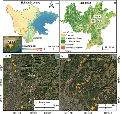
In China, Sichuan Province (Figure 1a) stands out as one of the provinces with the most abundant forest resources, characterized by exceptional carbon storage and huge carbon potential (Peng et al. 2023). Due to landscape heterogeneity and biodiversity, forest carbon monitoring requires accurate estimates of AGC at high resolution over large domains (W. Huang et al. 2019). This study was conducted in Liangshan Yi Autonomous Prefecture, Sichuan Province, China (Figure 1b). The study area is dominated by mountain and ravine areas with highly undulating, where altitudes vary from 305 to 5958 m above mean sea level. This area is located in the subtropical monsoon climate zone with an average annual temperature of 14.6°C and rainfall of 995.5 mm. The forest in the area is primarily dominated by evergreen coniferous forests (mainly Pinus Yunnanensis) (R. Chen et al. 2024) (Figure 1b).

Figure 1. Location of the study area; (a) the DEM of Sichuan Province (NASADEM (accessed via: https://www.earthdata.nasa.gov/esds/competitive-programs/measures/nasadem)); (b) the land-cover distributions of Liangshan Yi Autonomous Prefecture and the location of two field campaigns (GLC_FCS30, from Zhang et al. (2021b)); (c) geographic locations of sample plots in the first field campaign in December 2020; (d) geographic locations of sample plots in the second campaign in March 2021. The background map in subfigures (c-d) is from the Esri World Imagery (accessed via: https://www.arcgis.com/home/item.Html?id=10df2279f9684e4a9f6a7f08febac2a9).

2.2. Field data

To determine the locations of sample plots, we initially identified the principal representative Pinus Yunnanensis forestry areas within the study area. Subsequently, sample locations were randomly produced within each forestry area. However, due to the significant undulations in the terrain of the study area, many remote locations were excluded because forestry surveyors encountered difficulties in accessing them. Finally, the plots located in relatively homogeneous forest areas (>0.25 ha) were set. A total of 96 sample plots of Pinus Yunnanensis were acquired during two field campaigns conducted in Liangshan, sampling in December 2020 and March 2021(Figure 1c,d). Field data collection across all sites was consistently conducted using the following procedures. The sample plots were designed as 10 m × 10 m quadrats to be consistent with the spatial resolution of satellite images (Sentinel-1). Plot locations and in-field navigation were performed using a Global Positioning System (Trimble Geo 3000). Within these plots, trees with diameters at breast height (DBH) ≥ 5 cm were selected as samples. Their DBH was measured using a ruler, and tree height (H) was measured using a laser hypsometer device (Haglof Vertex Laser Geo). The aboveground biomass (AGB) was calculated based on measured factors using allometric equations previously developed for Pinus Yunnanensis (Eq. 1(1) $\mathit{AGB}=e^{-3.178+0.903\times ln(DB{H}^2\times \mathit{H})}-e^{-4.639+0.859\times ln(DB{H}^2\times \mathit{H})}$(1) ) (Ran et al. 2017). Forest AGC was then transformed from AGB by multiplying carbon content (CarbonContent=0.4947 for belowground biomass and 0.5106 for aboveground biomass) (Eq. 2(2) $\mathit{AGC}=\mathit{AGB}\times \mathit{CarbonContent}$(2) ), a constant measured by the National Forestry Administration of China (China 2014). Table 1 presents forest stand attribute statistics based on field surveys.

(1) $\mathit{AGB}=e^{-3.178+0.903\times ln(DB{H}^2\times \mathit{H})}-e^{-4.639+0.859\times ln(DB{H}^2\times \mathit{H})}$(1)

(2) $\mathit{AGC}=\mathit{AGB}\times \mathit{CarbonContent}$(2)

Table 1. Summary statistics of Pinus Yunnanensis in field plots in Liangshan, Sichuan.

Variables	AGB (Mg/ha)	AGC (Mg C/ha)	Mean DBH (cm)	Mean Height (m)	Tree density (N/ha)
Mean	140.257	71.615	22.1	12.4	1660
Minimum	2.692	1.375	9.6	4.7	20
Maximum	401.241	204.874	36.2	18.2	6800
S.D^.*	84.966	43.384	6.5	4.1	1108

*S.D. = standard deviation.

2.3. Remote sensing data

Time series of Landsat 8 Operational Land Imager (OLI) and Sentinel-1 dual-polarization C-band SAR (VV and VH polarizations) were employed in this study as they cover long periods. We obtained Landsat 8 (L8) atmospherically corrected (Level-2) surface reflectance data and Sentinel-1 (S1) Ground Range Detected (GRD) data from Google Earth Engine (GEE, https://earthengine.google.com/). Seven bands (B1 ~ 7) and five vegetation indices, including the Normalized Difference Vegetation Index (NDVI), Enhanced Vegetation Index (EVI), Ratio Vegetation Index (RVI), Global Vegetation Moisture Index (GVMI), Normalized Difference Infrared Index (NDII), were considered from L8 data (Table 2).

Table 2. The satellite-based time-series data used in this study.

Satellite	Time span	Variables	Descriptions
L8	April 2013 ~ March 2021	Band reflectance	B1 ~ 7
		NDVI	(NIR-R)/(NIR+R)
		EVI	2.5(NIR-Red)/(1+NIR+6Red-7.5Blue)
		RVI	NIR/Red
		GVMI	[(NIR+0.1)-(SWIR1+0.02)]/[(NIR+0.1)+ (SWIR1+0.02)]
		NDII	(NIR-SWIR2)/(NIR+SWIR2)
S1	April 2018 ~ March 2021	ASC_VV	-
		ASC_VH	-
		DESC_VV	-
		DESC_VH	-

All S1 images from GEE have been processed with thermal noise removal, radiometric calibration, speckle filtering (refined Lee filter) (J.-S. Lee 1981; Yommy, Liu, and Wu 2015), and geometric corrections (Range-Doppler terrain correction using SRTM 30) to reduce the undesirable image noise and terrain effects on image interpretation. The S1 SAR sensor looks at the ground from two orbit directions, i.e. ascending (ASC) and descending (DESC), which are observed in opposite directions. Previous studies have demonstrated that images acquired from different orbits contain different amounts of backscatter, resulting from several factors, including look direction, evapotranspiration, temperature, and water content of vegetation (Mahdavi, Amani, and Maghsoudi 2019; Sayedain, Maghsoudi, and Eini-Zinab 2020). Additionally, the S1 satellite passes over the study area at 11:15 ~ 11:17 UTM for the ASC orbit and at 23:04 ~ 23:15 UTM for the DESC orbit. The differences in orbit path and imaging time may affect the sensitivity of signal to vegetation structure (Bai et al. 2017). Therefore, treating the ASC and DESC time-series data separately helps improve data consistency and the effectiveness of temporal analysis (Bai et al. 2017; Y. X. Li et al. 2022). Consequently, we have extracted the backscatter coefficients of VV and VH from these separate datasets (i.e. ASC_VV, ASC_VH, DESC_VV, and DESC_VH). In addition, S1 images were resampled into a 30 m × 30 m resolution using the nearest neighbor algorithm to be consistent with the spatial resolution of L8 when mapping forest AGC.

Finally, 145 scenes of L8 were obtained from April 2013 to March 2021 after removing images severely polluted by clouds. 178 ASC and 183 DESC scenes of S1 were obtained from April 2018 to March 2021.

3. Methods

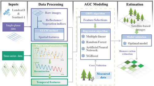
This section presents the method developed in this study for forest AGC estimation from L8 and S1 time-series data. In section 3.1, we described the pre-processing of time-series data and the algorithm of temporal feature extraction. In section 3.2, the method of spatial feature extraction was introduced. We finally explain the experimental design scheme and the procedures for developing the AGC models in section 3.3. Figure 2 visualizes the workflow of this method.

Figure 2. Methodology workflow for modeling forest AGC with L8 and S1 time-series data.

3.1. Temporal feature extraction

3.1.1. Time-series data reconstruction

Before temporal information extraction, the impact of forest disturbance and data gaps on the accuracy of temporal analysis is supposed to be reduced (Christ, Kempa-Liehr, and Feindt 2016; J. Zhang et al. 2021). First, we implemented the CCDC algorithm based on optical images to capture forest disturbance (Zhu and Woodcock 2014), and only stable time series (with no breakpoints) were used to analyze it further. Second, optical time series were reconstructed using the Harmonic (HR) model to fill data gaps caused by clouds and remove outliers. The HR model is an efficient reconstruction technique to model satellite time-series observations and reveal seasonal land surface dynamics (Y. X. Li et al. 2022; Zhou et al. 2022; Zhu et al. 2015). The HR model used to reconstruct time series was expressed:

(3) $\hat{p}(\mathit{i},\mathit{t})=c_{0,\mathit{i}}+c_{1,\mathit{i}}\mathit{t}\text{break}+{\sum }_{n=1}^N(a_{\mathit{n},\mathit{i}}cos\frac{2\mathit{\pi nt}}{T}+b_{\mathit{n},\mathit{i}}sin\frac{2\mathit{\pi nt}}{T})$(3)

where t, and i represent Julian date and the ith band. $\hat{p}\left(\mathit{i},\mathit{t}\right)$ is the predicted value for the ith band at a given Julian date t. c_0,i and c_1,i represent intercept and slope coefficients of the linear component, and a_n and b_n are n_th order seasonal harmonic coefficients. N is the temporal frequency of harmonic components indicating different forms, i.e. simple (N = 1), advanced (N = 2), and full (N = 3) model (Zhu et al. 2015), which was set to 3 in this study. n is the temporal frequency of the harmonic component. T is the number of days per year (set to be 365.25). The reconstructed time series was used to extract temporal features in the next step, and its length affects computational expense. Thus, after preliminary experiments, we observed that the 3-year reconstructed time series performed well, balancing model accuracy and efficiency. The SAR time-series data does not need to be reconstructed as it does not suffer from data gaps.

3.1.2. Temporal feature extraction

To utilize a set of time series as input for AGC modeling, each time series needs to be mapped into a well-defined feature space (Christ et al. 2018). A feature extraction algorithm of time-series data based on scalable hypothesis tests (tsfresh) was used to extract temporal features (Christ et al. 2018). The tsfresh algorithm combining 63 time-series characterization methods can compute 794 time-series features by default for each time series. In addition to features from the statistics domain, these temporal features are also derived from both the time domain and frequency domain, which can be effective in describing the rhythmic regularities in the time series (including the distribution of data points, stationarity, entropy, correlation properties, and nonlinear time-series analysis). They reflect the overall dynamics (the trend and periodic characteristics) of the time series, rather than information specific to a time point. Additionally, the tsfresh algorithm provides a preliminary feature selection module based on statistical hypothesis tests, removing irrelevant features depending on the specific application. This study considered 12 optical reconstructed time series from the HR model (Eq. 3(3) $\hat{p}(\mathit{i},\mathit{t})=c_{0,\mathit{i}}+c_{1,\mathit{i}}\mathit{t}\text{break}+{\sum }_{n=1}^N(a_{\mathit{n},\mathit{i}}cos\frac{2\mathit{\pi nt}}{T}+b_{\mathit{n},\mathit{i}}sin\frac{2\mathit{\pi nt}}{T})$(3) ) and four SAR observed time series to extract temporal features.

3.2. Spatial feature extraction

Texture features referring to the variance of pixel values associated with a particular object can characterize the structure properties and canopy complexity (Boyd and Danson 2005). Texture features were derived from satellite images close to field sampling time using Grey Level Co-occurrence Matrix (GLCM) methods, which described the relative frequency distribution of gray tones on the image (Conners, Trivedi, and Harlow 1984; Haralick, Shanmugam, and Dinstein 1973). To reduce the impact of window size on our experiments, all texture metrics were calculated at four offsets to generate eight features using four window sizes: 3 × 3, 5 × 5, 7 × 7, and 9 × 9 pixels (Kelsey and Neff 2014). We selected the best window size by comparing the correlations between texture features at different sizes and AGC.

3.3. Forest aboveground biomass carbon (AGC) estimation

3.3.1. Feature selection

Feature selection is a necessary procedure to remove unnecessary features and improve the algorithm’s work efficiency. The Gradient Boosted Feature Selection (GBFS) algorithm is scalable and straightforward to implement based on a variation of gradient boosting of limited depth trees (Friedman 2001), which can naturally discover nonlinear interactions between features (Natekin and Knoll 2013; Z. Xu et al. 2014). In addition, Xu et al. (2014) evaluated the GBFS algorithm on several real-world data sets and found it matched or outperformed the existing feature selection methods. Therefore, we performed the GBFS algorithm to select critical spatiotemporal features by changing thresholds representing absolute importance value.

3.3.2. Estimation algorithms

In this study, a parametric model (Multiple Linear Regression (MLR)) and three non-parametric models (Random Forest Regression (RF), eXtreme Gradient Boosting (XGBoost), and Artificial Neural Networks (ANN)) were performed to find connections between spatiotemporal features and AGC. The MLR model was widely used in forest variable predictions in previous studies with simple formulas and interpretability (Fang et al. 2023; D. S. Lu 2006). Previous study has indicated that collinearity among independent variables can lead to unreliable estimated parameters in MLR equations (Wooldridge 2012). Therefore, we conducted Variance Inflation Factor (VIF) tests to remove collinear variables before developing the MLR-based models. RF is a combination of tree predictors such that each tree depends on the values of a random sampled independently and with the same distribution for all trees in the forest (Breiman 2001), which has become popular within the remote sensing community due to the accuracy of its classifications and regressions (Belgiu and Drăguţ 2016; Quan, Xie, et al. 2021). XGBoost model is a novel sparsity-aware algorithm for sparse data and weighted quantile sketch for approximate tree learning based on tree boosting (T. Chen and Guestrin 2016; Friedman 2001). Unlike RF, where each tree is independent, XGBoost generates decision trees, with each tree depending on the others, and uses boosting and regulation techniques to reduce model variance (R. Chen et al. 2023; Friedman 2001; Lai et al. 2023). ANN, which can learn from data in hand without the need for data assumptions, has been utilized to find correlations between biophysical properties of forests and forest biomass carbon (G. J. Chang 2023; Domingues et al. 2020; Güner et al. 2022; Santi et al. 2017). An ANN comprises an input layer, one or more hidden layers, and one output layer (Güner et al. 2022). To best fit the ANN model, the proper net topology was specified for the case learning algorithm referring to Chang (2023) and Domingues et al. (2020). Due to limitations in the sample size required for deep learning-based methods, we have chosen an ANN model with three hidden layers, balancing model complexity and accuracy. The parameter tuning of each model was based on the grid search method (Z. Wu and Shi 2023; Yang et al. 2023). Previous studies have demonstrated that the tree-based method (including RF and XGBoost) worked reasonably well under moderate collinearity (R. Chen et al. 2023; Dormann et al. 2013), as did ANN approaches (Jensen, Qiu, and Ji 1999). We compared those four algorithms to find the optimal model for forest AGC estimation.

3.3.3. Experiment design

The experiments were designed to explore the potential of spatiotemporal characteristics for forest AGC estimation (Y. X. Li et al. 2022). According to different input feature groups representing different combinations of basic spectral response (including band reflectance and VIs) (R), spatial (S), and temporal (T) information, the input can be classified into nine experiments, as shown in Table 3. The Optical- experiments used only L8 observations. The SAR- experiments used only S1 observations. Based on the previous eight experiments, the OS-RST experiment combined L8 and S1 data. We initially employed the GBFS algorithm for feature selection in each experiment, followed by training AGC models with four regression algorithms.

Table 3. Model/Experimental setup to investigate the impacts of spatiotemporal features on AGC estimation.

Experiment/Model Label*	Feature group**	Num of features***
Optical -R	bands and VIs	12
Optical -RS	bands and VIs, and their spatial features	12+8*12
Optical -RT	bands and VIs, and their temporal features	12+400*12
Optical-RST	bands and VIs, and their spatiotemporal features	12+8*12+400*12
SAR-R	backscatter coefficients, including ASC_VV, ASC_VH, ASC_VV, DESC_VH	4
SAR-RS	4 backscatter coefficients, and their spatial features	4+8*4
SAR-RT	4 backscatter coefficients, and their temporal features	4+400*4
SAR-RST	4 backscatter coefficients, and their spatiotemporal features	4+8*4+400*4
OS-RST	all above features	12+8*12+400*12+(4+8*4+400*4)

*Optical-R and SAR-R represent spectral response information and backscatter coefficients from raw images. S and T mean spatial features and temporal features, respectively. **VIs indicate vegetation indices. The phrase “their temporal features” means the temporal features derived from the time series of spectral variables (including band reflectance, VIs, and backscatter coefficients). The phrase “their spatial features” means the spatial features derived from images of spectral variables. ***The number of temporal features extracted by the tsfresh algorithm is not constant, but approximately 400.

3.3.4. Accuracy assessment

Cross-validation is widely used in estimating vegetation proxies (Cui et al. 2023; Hiernaux et al. 2023), which can effectively select optimal models from a limited sample set with the best predictive ability and less overfitting (P. Zhang 1993). This study conducted tenfold cross-validation to optimize the configuration and evaluate the predictive performance of AGC models.

Three accuracy evaluation metrics were used to compare the performance of experiments and different models, including the determination coefficient (R²), the root mean square error (RMSE), and the relative root mean square error (rRMSE), as follows:

(4) $R^2=1-\frac{{\sum }_{i=1}^n{({\hat{y}}_{\mathit{i}}-\bar{y})}^2}{{\sum }_{i=1}^n{(y_i-\bar{y})}^2}$(4)

(5) $\mathit{RMSE}=\sqrt{\frac{1}{n}\sum _{\mathit{i}=1}^n(y_i-{\hat{y}}_{\mathit{i}})}$(5)

(6) $\mathit{rRMSE}=\frac{\mathit{RMSE}}{\bar{y}}$(6)

where n is the number of sample plots, y_i and ${\hat{y}}_{\mathit{i}}$ represent the ith measured and predicted AGC, respectively. $\bar{y}$ is the average of the measured AGC (i.e. y_i).

4. Result

4.1. Accuracy assessment of time-series data reconstruction

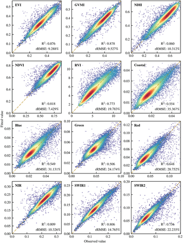
For optical observations, we first evaluated the reconstruction accuracy by comparing observed values with simulated values from the HR model (Eq. 3(3) $\hat{p}(\mathit{i},\mathit{t})=c_{0,\mathit{i}}+c_{1,\mathit{i}}\mathit{t}\text{break}+{\sum }_{n=1}^N(a_{\mathit{n},\mathit{i}}cos\frac{2\mathit{\pi nt}}{T}+b_{\mathit{n},\mathit{i}}sin\frac{2\mathit{\pi nt}}{T})$(3) ). Figure 3 illustrates the time-series reconstruction result, taking an in-situ plot as an example. The forest density in the plot gradually increases as time progresses from satellite images, with upward trends of the NIR band and vegetation indices and decreased trends of the Blue, Green, Red, and SWIR bands. Figure 4 shows the accuracy of HR model fitting, with all R² values exceeding 0.5 and rRMSE values below 30%. Especially for NIR, SWIR1, NDVI, EVI, GVMI, and NDII, R² values were over 0.8, and rRMSE values were below 15%. Overall, vegetation indices and spectral bands with strong surface reflection in forests (i.e. NIR, SWIR1, and SWIR2) exhibited better reconstruction performance. Those results suggest that the reconstructed time-series data is reliable for further temporal analysis.

Figure 3. The process of optical time-series reconstruction for a representative in-situ plot (with AGC of 24.67 Mg C/ha measured in November 2020). Gray spots are optical observations from Landsat 8. Blue dashed lines are fitted lines of the HR model. Orange lines are reconstructed time series. Historic satellite images of this plot came from Google Earth (access via https://earth.google.com/).

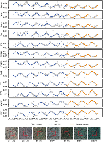
Figure 4. Scatterplots of HR model fitting. Observed values represent spectral reflections and vegetation indices, and fitted values represent predicted values from the HR model.

4.2. Accuracy comparison of machine learning algorithms

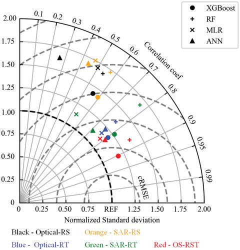
Four regression algorithms (i.e. MLR, RF, XGBoost, and ANN) were trained on different experiments (Table 2). Their performances were compared by the Taylor diagram (Figure 5) (Taylor 2001), according to metrics including normalized standard deviation, correlation coefficient, and centered root mean square error (cRMSE) (Zhou et al. 2021). We displayed five experimental outcomes (Optical-RS, SAR-RS, Optical-RT, SAR-RT, and OS-RTS) in Figure 5 since they can illustrate the overall situation. The MLR algorithm consistently showed substantial errors (correlation coefficient < 0.8) no matter which experiments, and their specific formulas were provided in Table S1 (see Supplementary). The RF algorithm exhibited large normalized standard deviations, indicating limited interpretability because the standard deviation of predicted values was less than the standard deviation of observed values. The performance of the ANN algorithm closely matched that of RF, with the additional advantage of exhibiting small normalized standard deviations. The XGBoost algorithm outperformed the other three algorithms with high correlation coefficients and low cRMSE values for different experiments. Therefore, we selected XGBoost to develop the AGC model and further analyzed the contribution of spatial and temporal features in the following sections.

Figure 5. Taylor diagram for accuracy comparison of different regression algorithms in different experiments. REF is the reference point, and cRMSE means the centred RMSE. The distance between the shape points and the REF point serves as an indicator of the models’ performances.

4.3. AGC estimation using single-sensor time-series data

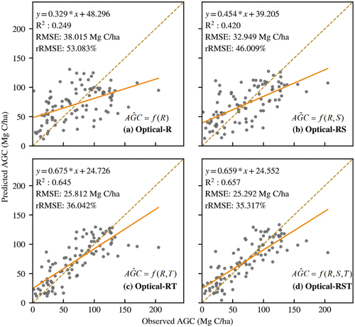
For using Landsat 8 alone, the model evaluation of different experiments (i.e. Optical-R, -RS, -RT, -RST) by relationships between predicted AGC and observed AGC are shown in Figure 6. The model performance was low when only using raw spectral responses from single-phase optical images (Figure 6a). With the addition of spatial features, the accuracy of AGC estimation improved, with R² increased by 0.171, RMSE decreased by 5.066 Mg C/ha, and rRMSE decreased by 7.074% (Figure 6b). The incorporation of temporal features resulted in a more remarkable improvement in accuracy compared to spatial features, with R² increased by 0.396, RMSE decreased by 12.203 Mg C/ha, and rRMSE decreased by 17.041% (Figure 6c). However, if spatial and temporal features are added simultaneously (i.e. Optical-RST), the model improvement was relatively limited compared to Optical-RT. Generally, from Optical-R to Optical-RST, a significant improvement in model performance was observed, and the slopes of fitted lines (orange lines in Figure 6a ~6d) have been improved from 0.329 to 0.659, indicating the mitigations of the underestimation of high-biomass forests and overestimation of low-biomass forests.

Figure 6. Scatter plots of AGC observation and prediction values from different experiments using optical time-series data. The formulas $\mathit{A}\hat{G}\mathit{C}=\mathit{f}\left(\right)$ in each subplot represent the AGC model.$\mathit{A}\hat{G}\mathit{C}$ is the predicted AGC.

For using SAR time-series data, the experimental results of the AGC estimation are shown in Figure 7. In the experiment SAR-R, only utilizing backscatter coefficients of raw images, the model performance was poor, even worse than in the experiment Optical-R. Compared with experiment SAR-R, adding temporal features much improved the model accuracy (R² increased by 0.553, rRMSE decreased by 22.159%) than adding spatial features (R² increased by 0.249, rRMSE decreased by 8.586%). When adding spatiotemporal features simultaneously (i.e. SAR-RST), the AGC estimation got high accuracy with R² of 0.672 and rRMSE of 34.701%. From SAR-R to SAR-RST, the slopes of fitted lines (orange lines in Figure 7a ~7d) have been improved from 0.140 to 0.625.

Figure 7. Scatter plots of AGC observation and prediction values from different experiments using SAR time-series data.

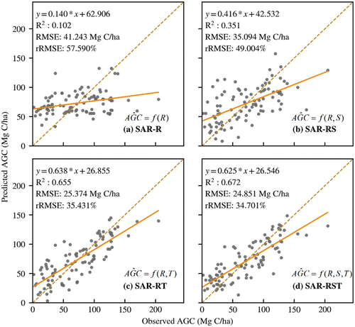
From both optical and SAR data, these results demonstrated that the temporal features were more valuable for AGC estimation than spatial features, accounting for around 40%~50% of the variance compared to 17%~25%.

4.4. AGC estimation using multi-sensor data and assessment of spatiotemporal features

Based on the above work, we further developed a model that combined time-series data of optical and SAR sensors. Figure 8 shows the feature selection process based on Gradient Boosted Feature Selection (GBFS) with different threshold values. Different feature combinations can be obtained by adjusting different algorithm thresholds, leading to varying performances of AGC estimation. As the GBFS threshold increases, the number of selected features gradually decreases, and the model performance initially improves before declining. Finally, the threshold value was determined to be 6, and a total of 18 features (shown in Figure 9a) were selected to develop the OS-RST model.

Figure 8. Feature selection process based on GBFS algorithm. Features whose absolute importance value ≥ the threshold value are selected. The number of selected features (a) and determination coefficient (R²) (b) of AGC estimation varied with the threshold value of GBFS.

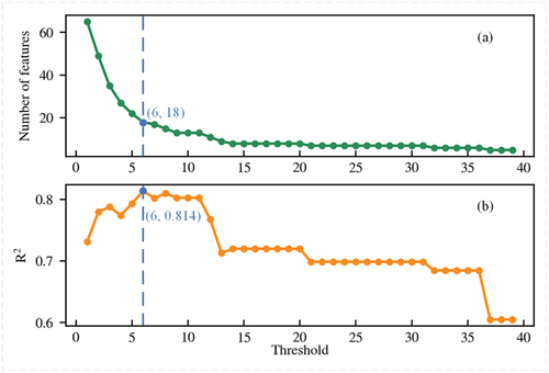
Figure 9. The importance of optical and SAR features (a), and the model performance of experiment OS-RST (b). Labels after bands or VIs represent the type of the features (temporal feature (_T)), and the phrase in parentheses were the specific calculation parameters. For instance, the feature “NDVI_T (cwt_coefficients_11)” represents the temporal feature (continuous wavelet transform (cwt), and the following number in brackets is the input parameter) of NDVI time-series data. The descriptions and calculations of selected features are shown in Table S2.

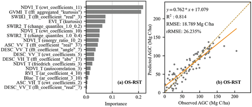
The OS-RST model achieved the best performance with R² of 0.814 and rRMSE of 26.235%, as shown in Figure 9b. In addition, the prediction saturation has been further mitigated, as evidenced by the increased slope of the fitted line (the orange line in Figure 9b) and good estimation for high AGC forests. These results demonstrated better performance of multi-sensor time-series data in AGC estimation than any single-sensor data. The feature importance of the OS-RST model is shown in Figure 9a. According to feature importance scores, temporal features are more critical for AGC estimation than spatial features, as GBFS selects no spatial features of either optical or SAR data. Specifically, the temporal features of NDVI, GVMI, EVI, RVI, SWIR, and Blue bands, as well as temporal features of dual-polarization backscatter signals, showed great potential for estimating AGC. The complementarity between optical and SAR time-series data was evident when evaluating the importance of selected features.

4.5. Applications in spatial forest carbon estimation

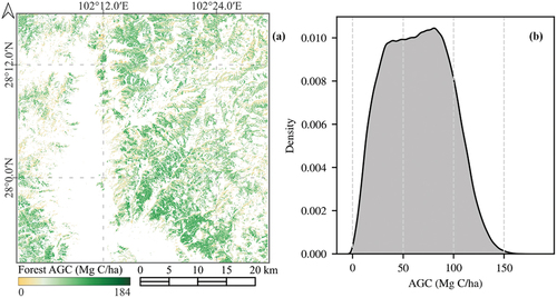
The AGC map in 2021 was generated using the OS-RST model (Figure 10). The AGC of evergreen coniferous forests was extracted using the land-cover product (GLC_FCS30) (X. Zhang et al. 2021), where AGC over the investigated area increased from slight yellow (0 Mg C/ha) to deep green (184 Mg C/ha). The predicted AGC was mainly concentrated in the range of 35 to 85 Mg C/ha, with an average of 64.33 Mg C/ha. The AGC map revealed the spatial heterogeneity patterns of forest AGC, which was characterized by higher AGC in the central and southern mountains while relatively lower AGC in the western and northeastern mountains. The blank in the central and southern plains correspond to cropland and towns.

Figure 10. Spatial distribution of evergreen coniferous forest AGC (a), and kernel density estimation of predicted AGC (b).

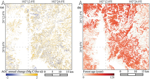
The AGC annual average change from 2016 to 2021 was estimated, as shown in Figure 11a. We noted that this map was produced from model Optical-RST (R² = 0.657 and rRMSE = 35.317%) rather than OS-RST because there is a massive gap of available Sentinel-1 GRD dual-polarization product in this study area from 2014 to 2016 (only four images from https://dataspace.copernicus.eu/), which cannot be used to calculate SAR temporal features required by OS-RST model. The estimated annual average change of AGC was +0.355 Mg C/(ha·a) in this region. Forests with carbon sinks accounted for 44.881% of total forests, and forests with stable carbon storage accounted for 30.989%. In addition, 24.130% of forests exhibited carbon sources. Those forests acting as carbon sources were primarily found in the central and southern regions characterized by relatively dense human populations.

Figure 11. (a) Estimation of forest AGC annual average changes in 2016—2021 and (b) forest stand age from the Forest Resource Inventory.

5. Discussion

5.1. Forest aboveground biomass carbon estimation

The study area is located on the edge of the Qinghai-Tibet Plateau, with rugged topography. Irregular terrain could affect pixel reflectance in remote sensing imagery (Jin et al. 2019), spatial heterogeneity of local climate (Çetin and Meydan 2023; Ogwang et al. 2014), and forest diversity and structure (Adams, Barnard, and Loomis 2014; Muscarella et al. 2020). These conditions increase the uncertainty of the remote sensing-based AGC estimation (W. Huang et al. 2010), causing relatively low accuracy using single-phase images, such as forest biomass models developed by Huang et al. (2023) and Zhang et al. (2022b) in southwestern China with similar topographical, climatological and phenological attributes as that of our study area. In this study, the proposed method utilized temporal features derived from satellite time-series data to capture the temporal dynamic changes of forests. Additionally, using time-series observations with varying solar zenith angles can mitigate the influence of terrain on AGC estimation. Hence, the models achieved high accuracy when employing optical or SAR time-series data alone (R² over 0.65, RMSE around 25 Mg C/ha, and rRMSE around 35%). The SAR-based method can be used alone to estimate AGC, giving results that are as satisfactory as the optical-based method when weather conditions are not ideal for optical sensor observation. Furthermore, the performance has been significantly improved when combining optical and SAR time-series data (R² = 0.814, RMSE = 18.789 Mg C/ha, rRMSE = 26.235%) because of the data complementarity of two sensors in characterizing forest properties.

The AGC of forests in the study area has exhibited an annual increase of 0.355 Mg C/(ha·a) from 2016 to 2021, indicating carbon sequestration. Previous research found that the carbon sink rate increases from young to middle age and then decreases (X. Li et al. 2023). Until the forest is over-mature, it is commonly assumed to be carbon neutral (Kenina et al. 2018; Seedre et al. 2015). From the forest stand age distribution based on the Forest Resource Inventory (Figure 11b), the average stand age was 44 years in this study area. When considering the age group structure, nearly 30% of forests were near-mature, with mature and over-mature forests accounting for 18.452% and 22.914%, respectively. The age structure of forests dominated by the mature stage resulted in quite a small annual average change of AGC. In spatially, over 75% of forests exhibited carbon sinks or stable carbon storage, suggesting that the implementation of ecological restoration programs has achieved initial success (such as the Natural Forest Protection Program and the Nature Reserve Development Program in Forestry Sector) (H. Wang et al. 2021; S. Wu et al. 2017). However, a small proportion of forests with carbon sources may be attributed to anthropogenic disturbances. De Marzo et al. (2023) demonstrated that anthropogenic disturbances had long-lasting effects on forests. Consequently, these regions need to improve forest protection, including establishing scientific, standardized, and systematic forest protection systems.

Despite the proposed method demonstrating exemplary performance in AGC estimation, there is a little saturation effect in high-biomass forests (AGC >150 Mg C/ha or AGB >300 Mg/ha) (Figure 9). The saturation effect varies with the complexity of forest landscape (e.g. forest structures and type) and spectral wavelengths (e.g. visible, near-infrared, short-wave infrared bands) (D. Lu and Jiang 2024; Zhao et al. 2016). The retrieved AGB from optical or short-wavelength microwave data always suffers from the saturation problem that the received signal no longer increases if the biomass is greater than a specific value due to the limited penetration ability of optical or microwave electromagnetic signals through the forest canopy (D. S. Lu et al. 2016; Yang et al. 2023). Previous studies have demonstrated that the PolInSAR and TomoSAR (Soja et al. 2021), LiDAR (Du et al. 2023), and optical stereoscopic imagery (Ni et al. 2023) can characterize the vertical structures of the forest canopy. Hence, the saturation problem in AGC estimation may be at least partly solved by incorporating the above data (Xiao et al. 2019). However, these data are not easy to obtain in practice applications. Currently, the PolInSAR, TomoSAR, and high point-density LiDAR data used in studies are mainly acquired by airborne sensors (Xiao et al. 2019) and high cost. In addition, the performances of methods using stereoscopic imagery are affected by several factors, such as sun elevation angle, seasonal variation, and forest phenology (Ni et al. 2023). In this study, employing satellite time-series data to estimate forest AGC is a low-cost and effective method to estimate forest biomass accurately, and our experiments have demonstrated that it can reduce the saturation effects.

5.2. Extensions of AGC models using time-series data

Some noticeable differences were found between the predicted AGC values from the four algorithms. This is due to different structures and principles of algorithms. The MLR algorithm is developed linearly, making it ineffective in explaining nonlinear relationships between AGC and the earth observation variables (David, Rosser, and Donoghue 2022). Machine learning techniques have the advantage of describing weak linear relationships between variables and biomass (Konya and Nematzadeh 2024; D. S. Lu et al. 2016), outperforming the MLR algorithm. The maximum predicted AGC from the RF-based model is always smaller than that from the XGBoost-based model; this is because the XGBoost algorithm is a scalable end-to-end tree boosting system that can achieve better accuracy than the RF algorithm (T. Chen and Guestrin 2016; R. Chen et al. 2023). Previous studies have demonstrated that deep learning-based methods are more effective in environmental applications than simple methods, offering new opportunities for ecological modeling, monitoring, and research (G. J. Chang 2023; Konya and Nematzadeh 2024). However, a notable challenge encountered in real-world scenarios requires a large amount of data during training (Konya and Nematzadeh 2024). In this study, the ANN algorithm did not perform as expected, which can be attributed to the constraint of sample size compared to the extensive parameter space. Grinsztajn et al. (2022) also showed that tree-based models outperformed deep learning on typical tabular data.

To further explore the performances of these algorithms, we consider two-way analysis of variance (ANOVA) to find the main effects and interaction effects of features and algorithms in AGC estimation (MacFarland 2011). Regardless of algorithms, the main effects of accounting for forest AGC estimation include the temporal features of NDVI, SWIR1/2, VV, and VH polarizations. The interaction effects between SAR signals and optical variables (especially for vegetation indices) showed significant importance for AGC estimation, also indicating the contributions of the complementarity between SAR and optical data. At the same time, there are differences between algorithms, manifested in the number of interaction effects. The XGBoost and ANN algorithms have more interaction effects than MLR and RF, and they perform well in AGC estimations. The details of ANOVA results are shown in Table S3 (in the Supplementary).

So far, some studies have explored the diverse forms of polarized radar signal responses to ecological properties and found that the single radar polarization parameter of cross-polarization showed good correlations with forest biomass (J. Chang and Shoshany 2017; Y. Wang et al. 1995). Interestingly, we found that the SAR backscatter temporal features from VV polarization are shown to be more important for the AGC estimations as compared to VH polarization (Figure 9a) in this study, consistent with the results obtained by Beaudoin et al. (1994) and David et al. (2022). This phenomenon may arise from several factors. Firstly, the sensitivity of VV/HH polarizations in SAR data to forest biomass varies with different wavelengths and forest structures (Sinha et al. 2015), and VV polarization showed strong correlations with tree height, diameters, and LAI (Wijaya et al. 2015). Additionally, the high correlation of VV polarization was probably due to ground backscatter signals as SAR also interacted with soil and litter biomass along with the tree canopy in the low-biomass forests (Sinha et al. 2018). Therefore, a small proportion of plots have very low forest AGC, making VV polarization more effective.

5.3. Contributions of spatiotemporal features to AGC estimation

We analyzed various experiment results and explored the contributions of temporal and spatial features to AGC estimation. The performance using raw information from single-phase images near field data collection was inferior. Although the addition of spatial features has improved the accuracy of AGC estimation, the application was still limited (Figures 5b and 6b). Texture information can indicate forest heterogeneity and homogeneity (Guerra-Hernández et al. 2022; Haralick, Shanmugam, and Dinstein 1973), which are associated with biological processes and population dynamics (Getzin et al. 2008), while its significance to biomass estimation varies with scales (Sarker et al. 2012; Xiao et al. 2019). However, due to the larger spatial resolution of images compared to the average tree size (DBH around 20 cm) in this study, texture features are difficult to provide refined canopy spatial information and might introduce noise. As a result, texture variables contained limited spatial information on the forest canopy, causing their notable absence from the feature importance ranking in the OS-RST model (Figure 9).

In contrast, temporal features were more valuable than spatial features for both sensor types, accounting for around 40%~50% of the variance compared to 17%~25%. Previous studies have demonstrated the validity of relationships between temporal features extracted from time-series images (as independent variables) and vegetation quantitative parameters at the final time step (as dependent variables) (Pötzschner et al. 2022; Travers-Smith et al. 2024). Its contribution to AGC estimation can be attributed to several factors. Fundamentally, the role of time-series information is related to forest growth curves (Forrester et al. 2017; Y. Zhang et al. 2022). Previous studies have revealed that the carbon sequestration rate of forests is a matter of tree age (N. P. He et al. 2017; Shang et al. 2023; H. Xu et al. 2023). The varied forest growth patterns result in differences in the optical reflectance or backscatter coefficient time series, leading to distinct temporal characteristics in the frequency domain and time domain (Brandes et al. 1968). Therefore, these temporal features, derived from the frequency domain and time domain by the tsfresh algorithm (such as parameters of Fourier transform and change quantiles), can capture the interannual and seasonal variations of photosynthetic phenology and water status in forests (Eitel et al. 2023). For example, in this study, the temporal variable “NDVI_T (cwt_ceoficients)” utilized in the OS-RST model, derived from the Continuous Wavelet Transform (Torrence and Compo 1998), can represent the overall level and internal fluctuation of NDVI time series. The larger “NDVI_T (cwt_coeficients),” the greater amplitude of internal fluctuations of NDVI over the time period, suggesting a higher AGC increment of the forest. Some temporal features can also reflect forest cover changes, such as “change_quantiles.” Additionally, temporal features can mitigate uncertainties from the diurnal variation in canopy water content (X. Xu et al. 2021), which may interfere with the AGC estimation based on single-phase water-sensitive signals like radar backscatter or short-wave infrared bands (Khabbazan et al. 2022; Y. X. Li et al. 2022). Due to the above advantages, the proposed method also mitigated the overestimation or underestimation of AGC.

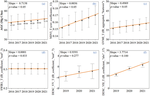
Furthermore, the changes and variations in forest estimated AGC and temporal features during 2016–2021 were analyzed, and their temporal trends are shown in Figure 12. SAR temporal features before 2019 were lacking due to the data gaps of Sentinel-1 in this study area. The estimated mean AGC of 96 plots increased from 67.35 Mg C/ha in 2016 to 71.53 Mg C/ha in 2021 (the average value of field-measured AGC is 71.62 Mg C/ha in 2021), demonstrating a significant increasing trend. Some temporal features (such as NDVI_T (cwt_coefficients) and DESC_VH_T (fft_coefficient)) also observed increasing trends over time, consistent with AGC. Also, some features did not exhibit a discernible increasing or decreasing trend (such as Figure 12d) due to the averaging of differences between plots. Hence, the variations of temporal features derived from L8 and S1 data can reflect the changes in forest AGC. The changes of other temporal features are shown in the Supplementary (Figure S1 and S2 in the Supplementary).

Figure 12. The changes in forest estimated AGC (a) and temporal features (b - f) during 2016 – 2021. The dark spots and gray bars represent mean values and 95% confidence intervals of AGC and feature in 96 plots, respectively. The orange lines described their temporal trends.

To explore the effects of time spans of time-series data on model performance, we have compared the performances of forest AGC models using several time-series data with different time spans (Table S4). The result showed that a larger time span of time-series data often results in better performance, consistent with Bolton et al. (2020). For optical data, the Optical-RT model performed well when the time span of the optical time-series data exceeded 2 years, with R² values over 0.6. However, the optical time-series reconstructions required a longer time span to enhance the effectiveness of reconstruction. For SAR data, the models performed well when using time-series data of more than 2 years, with R² values over 0.65. However, large time spans lead to increased computational costs. Consequently, selecting an appropriate time span of time series can ensure a balance between model performance and efficiency. When applying the proposed method to estimate forest AGC, it is recommended that the time span of time-series data should be determined based on the specific application context and the computational resources available.

5.4. Uncertainty and prospection in forest carbon monitoring

The main uncertainty among the forest AGC estimation using the proposed methods comes from several sources. (i) The uncertainty generated by the field measurements. The distribution of sample plots is not spatially uniform due to the significant terrain undulations in the study area, thereby influencing the representativeness of the samples. Additionally, variable measurements, particularly tree height, may experience a notable increase in errors within plots situated in complex terrains, such as steep slopes. (ii) The uncertainty generated by the satellite-based data. Regardless of optical or SAR data, topographic variances always affect the accuracy of optical or SAR calibration (Jin et al. 2019), even though images have been pre-processed with terrain correction step. (iii). The uncertainty generated by the model structure, including the error of time-series reconstruction and regression algorithms.

The C-band SAR data used in this study, which penetrates through leaves and is scattered by small branches and underlying features (Sinha et al. 2015), is less sensitive to forest structure information than longer wavelength SAR (L band and P band). If considering L-band SAR data, the proposed method’s performance can be further improved. Notably, our methodology needs to be validated over more forest types, particularly broadleaf forests. This is necessary because our experiments were exclusively conducted on coniferous forests (Pinus yunnanensis). Adapting this method for use with other forest types may require adjustments to account for varying environmental conditions and forest characteristics. Although the accuracy of forest AGC estimation in 2021 was significant, the error of predicting AGC in other years (past or future years) using the pre-trained model in this study may increase due to the limitation of field data (only including field data around 2021). We believe that the performance of AGC estimation in other years can be further improved if additional multi-year field data are incorporated. In addition, the relationship between temporal features and forest AGC is also worth exploring deeply.

6. Conclusions

This study has revealed the superiority of optical and SAR time-series data for the improvement of forest aboveground biomass carbon (AGC) estimation, which has been demonstrated in evergreen coniferous forests in Southwestern China. The temporal features were initially extracted from time-series data by data reconstructions and tsfresh algorithms. The XGBoost algorithm emerged as the most suitable method for estimating forest AGC with superior predictive accuracy and robust performance compared to the other three algorithms (i.e. MLR, RF, and ANN). Through experiments involving various combinations of spatial and temporal features, we found that adding temporal features can significantly improve accuracy in AGC estimation, outperforming spatial features, accounting for around 40%~50% of the variance compared to 17%~25%. When utilizing optical time-series data alone, the model achieved an R² of 0.657 and rRMSE of 35.317%, while when utilizing SAR time-series data alone, the R² was 0.672 and rRMSE was 34.701%. The synergistic use of optical and SAR time-series data produced the best performance (R² = 0.814, RMSE = 18.789 Mg C/ha, rRMSE = 26.235%). Furthermore, incorporating temporal features of optical and SAR data into the modeling was illustrated to effectively reduce saturation effects within high-biomass forests. These promising results warrant more research on the effectiveness of utilizing satellite time-series data for estimating AGC in other forest types not addressed in this study. Generally, the proposed methodology for AGC estimation carries significant implications for understanding the contribution of forests to the carbon cycle and supporting policy-making of forest management and sustainable development.

CRediT authorship contribution statement

Yiru Zhang: Conceptualization, Investigation, Methodology, Visualization, Writing – original draft. Binbin He: Conceptualization, Supervision, Writing- Reviewing and Editing. Rui Chen: Formal analysis, Validation, Writing- Reviewing and Editing. Hongguo Zhang: Methodology, Visualization, Writing- Reviewing and Editing. Chunquan Fan: Investigation, Writing- Reviewing and Editing. Jianpeng Yin: Visualization, Writing- Reviewing and Editing. Yanxi Li: Methodology, Writing- Reviewing and Editing.

Acknowledgments

The authors are grateful to (1) the Quantitative remote sensing team at the University of Electronic Science and Technology of China for the field data collection; (2) the USGS EROS Center for providing the Landsat 8 images; (3) the ESA for providing the Sentinel-1 images; and (4) the Sichuan Forestry and Grassland Administration for providing the forest resource survey data of Sichuan Province (2010–2020).

Disclosure statement

The authors declare that they have no known competing financial interests or personal relationships that could have appeared to influence the work reported in this paper.

Supplementary material

Supplemental data for this article can be accessed online at https://doi.org/10.1080/15481603.2024.2345438

Data availability statement

The Landsat data that support the findings of this study are available in the USGS EROS Center at https://earthexplorer.usgs.gov/. The Sentinel data are available in the ESA Copernicus Data Space Ecosystem at https://dataspace.copernicus.eu/.

Additional information

Funding

This work was supported by the National Key Research and Development Program of China [Contract No. 2022YFC3003001] and the Sichuan Science and Technology Program [Contract No. 2023YFS0432].

References

- Adams, H. R., H. R. Barnard, and A. K. Loomis. 2014. “Topography Alters Tree Growth–Climate Relationships in a Semi-Arid Forested Catchment.” Ecosphere 5 (11): 148. https://doi.org/10.1890/es14-00296.1.
- Askne, J. I. H., M. J. Soja, and L. M. H. Ulander. 2017. “Biomass Estimation in a Boreal Forest from TanDEM-X Data, Lidar DTM, and the Interferometric Water Cloud Model.” Remote Sensing of Environment 196:265–25. https://doi.org/10.1016/j.rse.2017.05.010.
- Baccini, A., W. Walker, L. Carvalho, M. Farina, D. Sulla-Menashe, and R. A. Houghton. 2017. “Tropical Forests Are a Net Carbon Source Based on Aboveground Measurements of Gain and Loss.” Science 358 (6360): 230–233. https://doi.org/10.1126/science.aam5962.
- Bai, X., B. He, X. Li, J. Zeng, X. Wang, Z. Wang, Y. Zeng, and Z. Su. 2017. “First Assessment of Sentinel-1A Data for Surface Soil Moisture Estimations Using a Coupled Water Cloud Model and Advanced Integral Equation Model Over the Tibetan Plateau.” Remote Sensing 9 (7): 714. https://doi.org/10.3390/rs9070714.
- Beaudoin, A., T. Le Toan, S. Goze, E. Nezry, A. Lopes, E. Mougin, C. C. Hsu, H. C. Han, J. A. Kong, and R. T. Shin. 1994. “Retrieval of Forest Biomass from SAR Data.” International Journal of Remote Sensing 15 (14): 2777–2796. https://doi.org/10.1080/01431169408954284.
- Beer, C., M. Reichstein, E. Tomelleri, P. Ciais, M. Jung, N. Carvalhais, C. Rödenbeck, et al. 2010. “Terrestrial Gross Carbon Dioxide Uptake: Global Distribution and Covariation with Climate.” Science 329 (5993): 834–838. https://doi.org/10.1126/science.1184984.
- Belgiu, M., and L. Drăguţ. 2016. “Random Forest in Remote Sensing: A Review of Applications and Future Directions.” Isprs Journal of Photogrammetry & Remote Sensing 114:24–31. https://doi.org/10.1016/j.isprsjprs.2016.01.011.
- Bolton, D. K., P. Tompalski, N. C. Coops, J. C. White, M. A. Wulder, T. Hermosilla, M. Queinnec, et al. 2020. “Optimizing Landsat Time Series Length for Regional Mapping of Lidar-Derived Forest Structure.” Remote Sensing of Environment 239:111645. https://doi.org/10.1016/j.rse.2020.111645.
- Boyd, D. S., and F. M. Danson. 2005. “Satellite Remote Sensing of Forest Resources: Three Decades of Research Development.” Progress in Physical Geography-Earth and Environment 29 (1): 1–26. https://doi.org/10.1191/0309133305pp432ra.
- Brandes, O., J. Farley, M. Hinich, and U. Zackrisson. 1968. “The Time Domain and the Frequency Domain in Time Series Analysis.” The Swedish Journal of Economics 70 (1): 25–42. https://doi.org/10.2307/3438983.
- Breiman, L. 2001. “Random Forests.” Machine Learning 45:5–32. https://doi.org/10.1023/A:1010933404324.
- Bustamante, M. M. C., I. Roitman, T. M. Aide, A. Alencar, L. O. Anderson, L. Aragao, G. P. Asner, et al. 2016. “Toward an Integrated Monitoring Framework to Assess the Effects of Tropical Forest Degradation and Recovery on Carbon Stocks and Biodiversity.” Global Change Biology 22 (1): 92–109. https://doi.org/10.1111/gcb.13087.
- Cao, M., and F. I. Woodward. 1998. “Dynamic Responses of Terrestrial Ecosystem Carbon Cycling to Global Climate Change.” Nature 393 (6682): 249–252. https://doi.org/10.1038/30460.
- Çetin, M., and A. Meydan. 2023. “Topography and Climate of Mount Karanfil (Pozantı/Adana).” Environmental Systems Research 12 (1): 1. https://doi.org/10.1186/s40068-022-00280-6.
- Chang, G. J. 2023. “Biodiversity Estimation by Environment Drivers Using Machine/Deep Learning for Ecological Management.” Ecological informatics 78:102319. https://doi.org/10.1016/j.ecoinf.2023.102319.
- Chang, J., and M. Shoshany. 2017. “Radar Polarization and Ecological Pattern Properties Across Mediterranean-To-Arid Transition Zone.” Remote Sensing of Environment 200:368–377. https://doi.org/10.1016/j.rse.2017.08.032.
- Chen, T., and C. Guestrin. 2016. “XGBoost.” In Proceedings of the 22nd ACM SIGKDD International Conference on Knowledge Discovery and Data Mining, San Francisco, CA, USA.
- Chen, R., B. B. He, Y. X. Li, C. Q. Fan, J. P. Yin, H. G. Zhang, and Y. R. Zhang. 2024. “Estimation of Potential Wildfire Behavior Characteristics to Assess Wildfire Danger in Southwest China Using Deep Learning Schemes.” Journal of Environmental Management 351. https://doi.org/10.1016/j.jenvman.2023.120005.
- Chen, R., B. B. He, X. W. Quan, X. Y. Lai, and C. Q. Fan. 2023. “Improving Wildfire Probability Modeling by Integrating Dynamic-Step Weather Variables Over Northwestern Sichuan, China.” International Journal of Disaster Risk Science 14:313–325. https://doi.org/10.1007/s13753-023-00476-z.
- Chen, J. M., W. Ju, P. Ciais, N. Viovy, R. Liu, Y. Liu, and X. Lu. 2019. “Vegetation Structural Change Since 1981 Significantly Enhanced the Terrestrial Carbon Sink.” Nature Communications 10 (1): 4259. https://doi.org/10.1038/s41467-019-12257-8.
- China, N. F. A. O. 2014. Tree Biomass Models and Related Parameters to Carbon Accounting for Pinus Yunnanensis. Beijing: Standards Press of China.
- Christ, M., N. Braun, J. Neuffer, and A. W. Kempa-Liehr. 2018. “Time Series FeatuRe Extraction on Basis of Scalable Hypothesis Tests (Tsfresh – a Python Package).” Neurocomputing 307:72–77. https://doi.org/10.1016/j.neucom.2018.03.067.
- Christ, M., A. Kempa-Liehr, and M. Feindt. 2016. “Distributed and Parallel Time Series Feature Extraction for Industrial Big Data Applications.” In The 8th Asian Conference on Machine Learning (ACML 2016), Hamilton, New Zealand.
- Conners, R. W., M. M. Trivedi, and C. A. Harlow. 1984. “Segmentation of a High-Resolution Urban Scene Using Texture Operators.” Computer Vision, Graphics and Image Processing 25 (3): 273–310. https://doi.org/10.1016/0734-189X(84)90197-X.
- Cui, T., L. Fan, P. Ciais, R. Fensholt, F. Frappart, S. Sitch, J. Chave, et al. 2023. “First Assessment of Optical and Microwave Remotely Sensed Vegetation Proxies in Monitoring Aboveground Carbon in Tropical Asia.” Remote Sensing of Environment 293:113619. https://doi.org/10.1016/j.rse.2023.113619.
- David, R. M., N. J. Rosser, and D. N. M. Donoghue. 2022. “Improving Above Ground Biomass Estimates of Southern Africa Dryland Forests by Combining Sentinel-1 SAR and Sentinel-2 Multispectral Imagery.” Remote Sensing of Environment 282:113232. https://doi.org/10.1016/j.rse.2022.113232.
- De Marzo, T., M. Pratzer, M. Baumann, N. I. Gasparri, F. Pötzschner, and T. Kuemmerle. 2023. “Linking Disturbance History to Current Forest Structure to Assess the Impact of Disturbances in Tropical Dry Forests.” Forest Ecology & Management 539:120989. https://doi.org/10.1016/j.foreco.2023.120989.
- Dixon, R. K., S. Brown, R. A. Houghton, A. M. Solomon, M. C. Trexler, and J. Wisniewski. 1994. “Carbon Pools and Flux of Global Forest Ecosystems.” Science 263 (5144): 185–190. https://doi.org/10.1126/science.263.5144.185.
- Domingues, G. F., V. P. Soares, H. G. Leite, A. S. Ferraz, C. A. A. S. Ribeiro, A. S. Lorenzon, G. E. Marcatti, et al. 2020. “Artificial Neural Networks on Integrated Multispectral and SAR Data for High-Performance Prediction of Eucalyptus Biomass.” Computers and Electronics in Agriculture 168:105089. https://doi.org/10.1016/j.compag.2019.105089.
- Dormann, C. F., J. Elith, S. Bacher, C. Buchmann, G. Carl, G. Carré, J. R. G. Marquéz, et al. 2013. “Collinearity: A Review of Methods to Deal with it and a Simulation Study Evaluating Their Performance.” Holarctic Ecology 36 (1): 27–46. https://doi.org/10.1111/j.1600-0587.2012.07348.x.
- Du, L., Y. Pang, Q. Wang, C. Huang, Y. Bai, D. Chen, W. Lu, and D. Kong. 2023. “A LiDAR Biomass Index-Based Approach for Tree- and Plot-Level Biomass Mapping Over Forest Farms Using 3D Point Clouds.” Remote Sensing of Environment 290. https://doi.org/10.1016/j.rse.2023.113543.
- Eitel, J. U. H., D. Basler, S. Braun, N. Buchmann, P. D’Odorico, S. Etzold, A. Gessler, et al. 2023. “Towards Monitoring Stem Growth Phenology from Space with High Resolution Satellite Data.” Agricultural and Forest Meteorology 339:109549. https://doi.org/10.1016/j.agrformet.2023.109549.
- Fang, G., H. Xu, S.-I. Yang, X. Lou, and L. Fang. 2023. “Synergistic Use of Sentinel-1, Sentinel-2, and Landsat 8 in Predicting Forest Variables.” Ecological Indicators 151:110296. https://doi.org/10.1016/j.ecolind.2023.110296.
- Forrester, D. I., I. H. H. Tachauer, P. Annighoefer, I. Barbeito, H. Pretzsch, R. Ruiz-Peinado, H. Stark, et al. 2017. “Generalized Biomass and Leaf Area Allometric Equations for European Tree Species Incorporating Stand Structure, Tree Age and Climate.” Forest Ecology & Management 396:160–175. https://doi.org/10.1016/j.foreco.2017.04.011.
- Friedman, J. H. 2001. “Greedy Function Approximation: A Gradient Boosting Machine.” Annals of Statistics 29 (5): 1189–1232. https://doi.org/10.1214/aos/1013203451.
- Getzin, S., T. Wiegand, K. Wiegand, and F. He. 2008. “Heterogeneity Influences Spatial Patterns and Demographics in Forest Stands.” The Journal of Ecology 96 (4): 807–820. https://doi.org/10.1111/j.1365-2745.2008.01377.x.
- Grinsztajn, L., E. Oyallon, and G. Varoquaux. 2022. “Why Do Tree-Based Models Still Outperform Deep Learning on Tabular Data?.” In 36th Conference on Neural Information Processing Sys- tems (NeurIPS 2022) Track on Datasets and Benchmarks, New Orleans, United States.
- Guerra-Hernández, J., L. L. Narine, A. Pascual, E. Gonzalez-Ferreiro, B. Botequim, L. Malambo, A. Neuenschwander, S. C. Popescu, and S. Godinho. 2022. “Aboveground Biomass Mapping by Integrating ICESat-2, SENTINEL-1, SENTINEL-2, ALOS2/PALSAR2, and Topographic Information in Mediterranean Forests.” GIScience & Remote Sensing 59 (1): 1509–1533. https://doi.org/10.1080/15481603.2022.2115599.
- Güner, Ş. T., M. J. Diamantopoulou, K. P. Poudel, A. Çömez, and R. Özçelik. 2022. “Employing Artificial Neural Network for Effective Biomass Prediction: An Alternative Approach.” Computers and Electronics in Agriculture 192:106596. https://doi.org/10.1016/j.compag.2021.106596.
- Haralick, R. M., K. Shanmugam, and I. Dinstein. 1973. “Textural Features for Image Classification.” IEEE Transactions on Systems, Man, and Cybernetics SMC-3 (6): 610–621. https://doi.org/10.1109/TSMC.1973.4309314.
- He, X., X. Lei, D. Liu, and Y. Lei. 2023. “Developing Machine Learning Models with Multiple Environmental Data to Predict Stand Biomass in Natural Coniferous-Broad Leaved Mixed Forests in Jilin Province of China.” Computers and Electronics in Agriculture 212:108162. https://doi.org/10.1016/j.compag.2023.108162.
- Herold, M., S. Carter, V. Avitabile, A. B. Espejo, I. Jonckheere, R. Lucas, R. E. Mcroberts, et al. 2019. “The Role and Need for Space-Based Forest Biomass-Related Measurements in Environmental Management and Policy.” Surveys in Geophysics 40 (4): 757–778. https://doi.org/10.1007/s10712-019-09510-6.
- He, N. P., D. Wen, J. X. Zhu, X. L. Tang, L. Xu, L. Zhang, H. F. Hu, M. Huang, and G. R. Yu. 2017. “Vegetation Carbon Sequestration in Chinese Forests from 2010 to 2050.” Global Change Biology 23 (4): 1575–1584. https://doi.org/10.1111/gcb.13479.
- Hiernaux, P., H. B.-A. Issoufou, C. Igel, A. Kariryaa, M. Kourouma, J. Chave, E. Mougin, and P. Savadogo. 2023. “Allometric Equations to Estimate the Dry Mass of Sahel Woody Plants Mapped with Very-High Resolution Satellite Imagery.” Forest Ecology & Management 529:120653. https://doi.org/10.1016/j.foreco.2022.120653.
- Houghton, R. A. 2005. “Aboveground Forest Biomass and the Global Carbon Balance.” Global Change Biology 11 (6): 945–958. https://doi.org/10.1111/j.1365-2486.2005.00955.x.
- Huang, W., K. Dolan, A. Swatantran, K. Johnson, H. Tang, J. O’Neil-Dunne, R. Dubayah, and G. Hurtt. 2019. “High-Resolution Mapping of Aboveground Biomass for Forest Carbon Monitoring System in the Tri-State Region of Maryland, Pennsylvania and Delaware, USA.” Environmental Research Letters 14:095002. https://doi.org/10.1088/1748-9326/ab2917.
- Huang, T., G. Ou, Y. Wu, X. Zhang, Z. Liu, H. Xu, X. Xu, Z. Wang, and C. Xu. 2023. “Estimating the Aboveground Biomass of Various Forest Types with High Heterogeneity at the Provincial Scale Based on Multi-Source Data.” Remote Sensing 15 (14): 3550. https://doi.org/10.3390/rs15143550.
- Huang, W., L. Zhang, S. Furumi, K. Muramatsu, M. Daigo, and P. Li. 2010. “Topographic Effects on Estimating Net Primary Productivity of Green Coniferous Forest in Complex Terrain Using Landsat Data: A Case Study of Yoshino Mountain, Japan.” International Journal of Remote Sensing 31 (11): 2941–2957. https://doi.org/10.1080/01431160903140829.
- Jensen, J. R., F. Qiu, and M. H. Ji. 1999. “Predictive Modelling of Coniferous Forest Age Using Statistical and Artificial Neural Network Approaches Applied to Remote Sensor Data.” International Journal of Remote Sensing 20 (14): 2805–2822. https://doi.org/10.1080/014311699211804.
- Jin, H., A. Li, W. Xu, Z. Xiao, J. Jiang, and H. Xue. 2019. “Evaluation of Topographic Effects on Multiscale Leaf Area Index Estimation Using Remotely Sensed Observations from Multiple Sensors.” Isprs Journal of Photogrammetry & Remote Sensing 154:176–188. https://doi.org/10.1016/j.isprsjprs.2019.06.008.
- Kelsey, K., and J. Neff. 2014. “Estimates of Aboveground Biomass from Texture Analysis of Landsat Imagery.” Remote Sensing 6 (7): 6407–6422. https://doi.org/10.3390/rs6076407.
- Kenina, L., D. Elferts, E. Baders, and A. Jansons. 2018. “Carbon Pools in a Hemiboreal Over-Mature Norway Spruce Stands.” FORESTS 9 (7): 435. https://doi.org/10.3390/f9070435.
- Khabbazan, S., S. C. Steele-Dunne, P. Vermunt, J. Judge, M. Vreugdenhil, and G. Gao. 2022. “The Influence of Surface Canopy Water on the Relationship Between L-Band Backscatter and Biophysical Variables in Agricultural Monitoring.” Remote Sensing of Environment 268:112789. https://doi.org/10.1016/j.rse.2021.112789.
- Konya, A., and P. Nematzadeh. 2024. “Recent Applications of AI to Environmental Disciplines: A Review.” Science of the Total Environment 906:167705. https://doi.org/10.1016/j.scitotenv.2023.167705.
- Lai, L., Y. Zhang, Z. Cao, Z. Liu, and Q. Yang. 2023. “Algal Biomass Mapping of Eutrophic Lakes Using a Machine Learning Approach with MODIS Images.” Science of the Total Environment 880:163357. https://doi.org/10.1016/j.scitotenv.2023.163357.
- Larocque, G. R., J. S. Bhatti, R. Boutin, and O. Chertov. 2008. “Uncertainty Analysis in Carbon Cycle Models of Forest Ecosystems: Research Needs and Development of a Theoretical Framework to Estimate Error Propagation.” Ecological Modelling 219 (3): 400–412. https://doi.org/10.1016/j.ecolmodel.2008.07.024.
- Lee, J.-S. 1981. “Refined Filtering of Image Noise Using Local Statistics.” Computer Graphics and Image Processing 15 (4): 380–389. https://doi.org/10.1016/S0146-664X(81)80018-4.
- Lee, J. S., L. Jurkevich, P. Dewaele, P. Wambacq, and A. Oosterlinck. 1994. “Speckle Filtering of Synthetic Aperture Radar Images: A Review.” Remote sensing reviews 8 (4): 313–340. https://doi.org/10.1080/02757259409532206.
- Li, X., L. C. R. Aguila, D. H. Wu, Z. Lie, W. F. Xu, X. L. Tang, and J. X. Liu. 2023. “Carbon Sequestration and Storage Capacity of Chinese Fir at Different Stand Ages.” Science of the Total Environment 904:166962. https://doi.org/10.1016/j.scitotenv.2023.166962.
- Liao, Z., B. He, X. Quan, A. I. J. M. van Dijk, S. Qiu, and C. Yin. 2019. “Biomass Estimation in Dense Tropical Forest Using Multiple Information from Single-Baseline P-Band PolInSAR Data.” Remote Sensing of Environment 221:489–507. https://doi.org/10.1016/j.rse.2018.11.027.
- Liao, Z., X. Liu, A. van Dijk, C. Yue, and B. He. 2022. “Continuous Woody Vegetation Biomass Estimation Based on Temporal Modeling of Landsat Data.” International Journal of Applied Earth Observation and Geoinformation 110:102811. https://doi.org/10.1016/j.jag.2022.102811.
- Li, Y. X., R. Chen, B. B. He, and S. Veraverbeke. 2022. “Forest Foliage Fuel Load Estimation from Multi-Sensor Spatiotemporal Features.” International Journal of Applied Earth Observation and Geoinformation 115:103101. https://doi.org/10.1016/j.jag.2022.103101.
- Li, X., J. Xiao, B. He, M. Altaf Arain, J. Beringer, A. R. Desai, C. Emmel, et al. 2018. “Solar-Induced Chlorophyll Fluorescence Is Strongly Correlated with Terrestrial Photosynthesis for a Wide Variety of Biomes: First Global Analysis Based on OCO-2 and Flux Tower Observations.” Glob Chang Biol 24 (9): 3990–4008. https://doi.org/10.1111/gcb.14297.
- Lu, D. S. 2006. “The Potential and Challenge of Remote Sensing-Based Biomass Estimation.” International Journal of Remote Sensing 27 (7): 1297–1328. https://doi.org/10.1080/01431160500486732.
- Lu, D. S., Q. Chen, G. X. Wang, L. J. Liu, G. Y. Li, and E. Moran. 2016. “A Survey of Remote Sensing-Based Aboveground Biomass Estimation Methods in Forest Ecosystems.” International Journal of Digital Earth 9 (1): 63–105. https://doi.org/10.1080/17538947.2014.990526.
- Lu, D., and X. Jiang. 2024. “A Brief Overview and Perspective of Using Airborne Lidar Data for Forest Biomass Estimation.” International Journal of Image and Data Fusion 15 (1): 1–24. https://doi.org/10.1080/19479832.2024.2309615.
- Lu, J. B., H. Wang, S. H. Qin, L. Cao, R. L. Pu, G. L. Li, and J. Sun. 2020. “Estimation of Aboveground Biomass of Robinia pseudoacacia Forest in the Yellow River Delta Based on UAV and Backpack LiDAR Point Clouds.” International Journal of Applied Earth Observation and Geoinformation 86. https://doi.org/10.1016/j.jag.2019.102014.
- MacFarland, T. W. 2011. Two-Way Analysis of Variance: Statistical Tests and Graphics Using R. 1st ed. New York, NY, USA: Springer. https://doi.org/10.1007/978-1-4614-2134-4.
- Mahdavi, S., M. Amani, and Y. Maghsoudi. 2019. “The Effects of Orbit Type on Synthetic Aperture RADAR (SAR) Backscatter.” Remote Sensing Letters 10 (2): 120–128. https://doi.org/10.1080/2150704X.2018.1530481.
- Morecroft, M. D., S. Duffield, M. Harley, J. W. Pearce-Higgins, N. Stevens, O. Watts, and J. Whitaker. 2019. “Measuring the Success of Climate Change Adaptation and Mitigation in Terrestrial Ecosystems.” Science 366:eaaw9256. https://doi.org/10.1126/science.aaw9256.
- Muscarella, R., S. Kolyaie, D. C. Morton, J. K. Zimmerman, and M. Uriarte. 2020. “Effects of Topography on Tropical Forest Structure Depend on Climate Context.” The Journal of Ecology 108 (1): 145–159. https://doi.org/10.1111/1365-2745.13261.
- Natekin, A., and A. Knoll. 2013. “Gradient Boosting Machines, a Tutorial.” Frontiers in Neurorobotics 7:21. https://doi.org/10.3389/fnbot.2013.00021.
- Ni, W., T. Yu, Y. Pang, Z. Zhang, Y. He, Z. Li, and G. Sun. 2023. “Seasonal Effects on Aboveground Biomass Estimation in Mountainous Deciduous Forests Using ZY-3 Stereoscopic Imagery.” Remote Sensing of Environment 289. https://doi.org/10.1016/j.rse.2023.113520.
- Ogwang, B. A., H. Chen, X. Li, and C. Gao. 2014. “The Influence of Topography on East African October to December Climate: Sensitivity Experiments with RegCm4.” Advances in Meteorology 2014:143917. https://doi.org/10.1155/2014/143917.
- Pan, Y. D., R. A. Birdsey, J. Y. Fang, R. Houghton, P. E. Kauppi, W. A. Kurz, O. L. Phillips, et al. 2011. “A Large and Persistent Carbon Sink in the world’s Forests.” Science 333 (6045): 988–993. https://doi.org/10.1126/science.1201609.
- Peng, B., Z. Zhou, W. Cai, M. Li, L. Xu, and N. He. 2023. “Maximum Potential of Vegetation Carbon Sink in Chinese Forests.” Science of the Total Environment 905:167325. https://doi.org/10.1016/j.scitotenv.2023.167325.
- Piao, S. L., J. Y. Fang, P. Ciais, P. Peylin, Y. Huang, S. Sitch, and T. Wang. 2009. “The Carbon Balance of Terrestrial Ecosystems in China.” Nature 458 (7241): 1009–1013. https://doi.org/10.1038/nature07944.
- Pötzschner, F., M. Baumann, N. I. Gasparri, G. Conti, D. Loto, M. Piquer-Rodríguez, and T. Kuemmerle. 2022. “Ecoregion-Wide, Multi-Sensor Biomass Mapping Highlights a Major Underestimation of Dry Forests Carbon Stocks.” Remote Sensing of Environment 269:112849. https://doi.org/10.1016/j.rse.2021.112849.
- Qi, Z., S. Li, Y. Pang, L. Du, H. Zhang, and Z. Li. 2023. “Monitoring Spatiotemporal Variation of Individual Tree Biomass Using Multitemporal LiDAR Data.” Remote Sensing 15 (19): 4768. https://doi.org/10.3390/rs15194768.
- Quan, X., Y. Li, B. He, G. J. Cary, and G. Lai. 2021. “Application of Landsat ETM+ and OLI Data for Foliage Fuel Load Monitoring Using Radiative Transfer Model and Machine Learning Method.” IEEE Journal of Selected Topics in Applied Earth Observations & Remote Sensing 14:5100–5110. https://doi.org/10.1109/jstars.2021.3062073.
- Quan, X., Q. Xie, B. He, K. Luo, and X. Liu. 2021. “Integrating Remotely Sensed Fuel Variables into Wildfire Danger Assessment for China.” International Journal of Wildland Fire 30 (10): 807–821. https://doi.org/10.1071/wf20077.
- Ramachandran, N., S. Saatchi, S. Tebaldini, M. M. D’Alessandro, and O. Dikshit. 2023. “Mapping Tropical Forest Aboveground Biomass Using Airborne SAR Tomography.” Scientific Reports 13 (1): 6233. https://doi.org/10.1038/s41598-023-33311-y.
- Ran, F., R.-Y. Chang, Y. Yang, W.-Z. Zhu, J. Luo, and G.-X. Wang. 2017. “Allometric Equations of Select Tree Species of the Tibetan Plateau, China.” Journal of Mountain Science 14 (9): 1889–1902. https://doi.org/10.1007/s11629-016-4082-4.
- Rodríguez-Fernández, N. J., A. Mialon, S. Mermoz, A. Bouvet, P. Richaume, A. Al Bitar, A. Al-Yaari, et al. 2018. “An Evaluation of SMOS L-Band Vegetation Optical Depth (L-VOD) Data Sets: High Sensitivity of L-VOD to Above-Ground Biomass in Africa.” Biogeosciences 15 (14): 4627–4645. https://doi.org/10.5194/bg-15-4627-2018.
- Santi, E., S. Paloscia, S. Pettinato, G. Fontanelli, M. Mura, C. Zolli, F. Maselli, M. Chiesi, L. Bottai, and G. Chirici. 2017. “The Potential of Multifrequency SAR Images for Estimating Forest Biomass in Mediterranean Areas.” Remote Sensing of Environment 200:63–73. https://doi.org/10.1016/j.rse.2017.07.038.
- Sarker, M. L. R., J. Nichol, B. Ahmad, I. Busu, and A. A. Rahman. 2012. “Potential of Texture Measurements of Two-Date Dual Polarization PALSAR Data for the Improvement of Forest Biomass Estimation.” Isprs Journal of Photogrammetry & Remote Sensing 69:146–166. https://doi.org/10.1016/j.isprsjprs.2012.03.002.
- Sayedain, S. A., Y. Maghsoudi, and S. Eini-Zinab. 2020. “Assessing the Use of Cross-Orbit Sentinel-1 Images in Land Cover Classification.” International Journal of Remote Sensing 41 (20): 7801–7819. https://doi.org/10.1080/01431161.2020.1763512.
- Seedre, M., J. Kopácek, P. Janda, R. Bace, and M. Svoboda. 2015. “Carbon Pools in a Montane Old-Growth Norway Spruce Ecosystem in Bohemian Forest: Effects of Stand Age and Elevation.” Forest Ecology & Management 346:106–113. https://doi.org/10.1016/j.foreco.2015.02.034.
- Shang, R., J. M. Chen, M. Xu, X. Lin, P. Li, G. Yu, N. He, et al. 2023. “China’s Current Forest Age Structure Will Lead to Weakened Carbon Sinks in the Near Future.” The Innovation 4 (6): 100515. https://doi.org/10.1016/j.xinn.2023.100515.
- Singh, C., S. K. Karan, P. Sardar, and S. R. Samadder. 2022. “Remote Sensing-Based Biomass Estimation of Dry Deciduous Tropical Forest Using Machine Learning and Ensemble Analysis.” Journal of Environmental Management 308:114639. https://doi.org/10.1016/j.jenvman.2022.114639.
- Sinha, S., C. Jeganathan, L. K. Sharma, and M. S. Nathawat. 2015. “A Review of Radar Remote Sensing for Biomass Estimation.” International Journal of Environmental Science and Technology 12 (5): 1779–1792. https://doi.org/10.1007/s13762-015-0750-0.
- Sinha, S., A. Santra, L. Sharma, C. Jeganathan, M. S. Nathawat, A. K. Das, and S. Mohan. 2018. “Multi-Polarized Radarsat-2 Satellite Sensor in Assessing Forest Vigor from Above Ground Biomass.” Journal of Forestry Research 29 (4): 1139–1145. https://doi.org/10.1007/s11676-017-0511-7.
- Soja, M. J., S. Quegan, M. M. d’Alessandro, F. Banda, K. Scipal, S. Tebaldini, and L. M. H. Ulander. 2021. “Mapping Above-Ground Biomass in Tropical Forests with Ground-Cancelled P-Band SAR and Limited Reference Data.” Remote Sensing of Environment 253:112153. https://doi.org/10.1016/j.rse.2020.112153.
- Taylor, K. E. 2001. “Summarizing Multiple Aspects of Model Performance in a Single Diagram.” Journal of Geophysical Research-Atmospheres 106 (D7): 7183–7192. https://doi.org/10.1029/2000jd900719.
- Thurner, M., C. Beer, M. Santoro, N. Carvalhais, T. Wutzler, D. Schepaschenko, A. Shvidenko, et al. 2014. “Carbon Stock and Density of Northern Boreal and Temperate Forests.” Global Ecology & Biogeography 23 (3): 297–310. https://doi.org/10.1111/geb.12125.
- Torrence, C., and G. P. Compo. 1998. “A Practical Guide to Wavelet Analysis.” Bulletin of the American Meteorological Society 79 (1): 61–78. https://doi.org/10.1175/1520-0477(1998)079<0061:APGTWA>2.0.CO;2.
- Travers-Smith, H., N. C. Coops, C. Mulverhill, M. A. Wulder, D. Ignace, and T. C. Lantz. 2024. “Mapping Vegetation Height and Identifying the Northern Forest Limit Across Canada Using ICESat-2, Landsat Time Series and Topographic Data.” Remote Sensing of Environment 305:114097. https://doi.org/10.1016/j.rse.2024.114097.
- Wang, Y., F. W. Davis, J. M. Melack, E. S. Kasischke, and N. L. Christensen Jr. 1995. “The Effects of Changes in Forest Biomass on Radar Backscatter from Tree Canopies.” International Journal of Remote Sensing 16 (3): 503–513. https://doi.org/10.1080/01431169508954415.
- Wang, H., M. He, N. Ran, D. Xie, Q. Wang, M. Teng, and P. Wang. 2021. “China’s Key Forestry Ecological Development Programs: Implementation, Environmental Impact and Challenges.” FORESTS 12 (1): 101. https://doi.org/10.3390/f12010101.
- Wang, J., F. Jiang, H. Wang, B. Qiu, M. Wu, W. He, W. Ju, Y. Zhang, J. M. Chen, and Y. Zhou. 2021. “Constraining Global Terrestrial Gross Primary Productivity in a Global Carbon Assimilation System with OCO-2 Chlorophyll Fluorescence Data.” Agricultural and Forest Meteorology 304-305:108424. https://doi.org/10.1016/j.agrformet.2021.108424.
- West, P. W. 2015. Tree and Forest Measurement. 3rd ed. Cham, Switzerland: Springer. https://doi.org/10.1007/978-3-319-14708-6.
- Wijaya, A., V. Liesenberg, A. Susanti, O. Karyanto, and L. V. Verchot. 2015. “Estimation of Biomass Carbon Stocks Over Peat Swamp Forests Using Multi-Temporal and Multi-Polratizations SAR Data.” International Archives of the Photogrammetry, Remote Sensing and Spatial Information Sciences 551–556. https://doi.org/10.5194/isprsarchives-xl-7-w3-551-2015.
- Wooldridge, J. M. 2012. Introductory Econometrics: A Modern Approach. 5th ed. Mason, OH, USA: Cengage Learning.
- Wu, S., J. Li, W. Zhou, B. J. Lewis, D. Yu, L. Zhou, L. Jiang, and L. Dai. 2017. “A Statistical Analysis of Spatiotemporal Variations and Determinant Factors of Forest Carbon Storage Under China’s Natural Forest Protection Program.” Journal of Forestry Research 29 (2): 415–424. https://doi.org/10.1007/s11676-017-0462-z.
- Wu, Z., and F. Shi. 2023. “Mapping Forest Canopy Height at Large Scales Using ICESat-2 and Landsat: An Ecological Zoning Random Forest Approach.” IEEE Transactions on Geoscience & Remote Sensing 61:1–16. https://doi.org/10.1109/tgrs.2022.3231926.
- Xiao, J., F. Chevallier, C. Gomez, L. Guanter, J. A. Hicke, A. R. Huete, K. Ichii, et al. 2019. “Remote Sensing of the Terrestrial Carbon Cycle: A Review of Advances Over 50 Years.” Remote Sensing of Environment 233:111383. https://doi.org/10.1016/j.rse.2019.111383.
- Xu, Z., G. Huang, K. Q. Weinberger, and A. X. Zheng. 2014. “Gradient Boosted Feature Selection.” In Proceedings of the 20th ACM SIGKDD international conference on Knowledge discovery and data mining, New York, NY, USA.
- Xu, X., A. G. Konings, M. Longo, A. Feldman, L. Xu, S. Saatchi, D. Wu, J. Wu, and P. Moorcroft. 2021. “Leaf Surface Water, Not Plant Water Stress, Drives Diurnal Variation in Tropical Forest Canopy Water Content.” The New Phytologist 231 (1): 122–136. https://doi.org/10.1111/nph.17254.
- Xu, H., C. Yue, Y. Zhang, D. Liu, and S. Piao. 2023. “Forestation at the Right Time with the Right Species Can Generate Persistent Carbon Benefits in China.” Proceedings of the National Academy of Sciences 120 (41): e2304988120. https://doi.org/10.1073/pnas.2304988120.
- Yang, Q., C. Niu, X. Liu, Y. Feng, Q. Ma, X. Wang, H. Tang, and Q. Guo. 2023. “Mapping High-Resolution Forest Aboveground Biomass of China Using Multisource Remote Sensing Data.” GIScience & Remote Sensing 60 (1): 2203303. https://doi.org/10.1080/15481603.2023.2203303.
- Yommy, A. S., R. Liu, and A. S. Wu. 2015. “SAR Image Despeckling Using Refined Lee Filter.“ In 2015 7th International Conference on Intelligent Human-Machine Systems and Cybernetics, Hangzhou, China.
- Zhang, P. 1993. “Model Selection via Multifold Cross Validation.” Annals of Statistics 21 (1): 299–313. https://doi.org/10.1214/aos/1176349027.
- Zhang, X., L. Liu, X. Chen, Y. Gao, S. Xie, and J. Mi. 2021. “GLC_FCS30: Global Land-Cover Product with Fine Classification System at 30 m Using Time-Series Landsat Imagery.” Earth System Science Data 13 (6): 2753–2776. https://doi.org/10.5194/essd-13-2753-2021.
- Zhang, Y., H. Li, X. Zhang, Y. Lei, J. Huang, and X. Liu. 2022. “An Approach to Estimate Individual Tree Ages Based on Time Series Diameter Data—A Test Case for Three Subtropical Tree Species in China.” FORESTS 13 (4): 614. https://doi.org/10.3390/f13040614.
- Zhang, J., R. Shang, C. Rittenhouse, C. Witharana, and Z. Zhu. 2021. “Evaluating the Impacts of Models, Data Density and Irregularity on Reconstructing and Forecasting Dense Landsat Time Series.” Science of Remote Sensing 4:100023. https://doi.org/10.1016/j.srs.2021.100023.
- Zhang, F. Y., X. Tian, H. B. Zhang, and M. Jiang. 2022. “Estimation of Aboveground Carbon Density of Forests Using Deep Learning and Multisource Remote Sensing.” Remote Sensing 14 (13): 3022. https://doi.org/10.3390/rs14133022.
- Zhang, Y., N. Wang, Y. Wang, and M. Li. 2023. “A New Strategy for Improving the Accuracy of Forest Aboveground Biomass Estimates in an Alpine Region Based on Multi-Source Remote Sensing.” GIScience & Remote Sensing 60 (1): 2163574. https://doi.org/10.1080/15481603.2022.2163574.
- Zhang, W., L. Zhao, Y. Li, J. Shi, M. Yan, and Y. Ji. 2022. “Forest Above-Ground Biomass Inversion Using Optical and SAR Images Based on a Multi-Step Feature Optimized Inversion Model.” Remote Sensing 14 (7): 1608. https://doi.org/10.3390/rs14071608.
- Zhao, P., D. Lu, G. Wang, C. Wu, Y. Huang, and S. Yu. 2016. “Examining Spectral Reflectance Saturation in Landsat Imagery and Corresponding Solutions to Improve Forest Aboveground Biomass Estimation.” Remote Sensing 8 (6). https://doi.org/10.3390/rs8060469.
- Zhou, Q., D. Chen, Z. Hu, and X. Chen. 2021. “Decompositions of Taylor Diagram and DISO Performance Criteria.” International Journal of Climatology 41:5726–5732. https://doi.org/10.1002/joc.7149.
- Zhou, Q., Z. Zhu, G. Xian, and C. Li. 2022. “A Novel Regression Method for Harmonic Analysis of Time Series.” Isprs Journal of Photogrammetry & Remote Sensing 185:48–61. https://doi.org/10.1016/j.isprsjprs.2022.01.006.
- Zhu, Z., and C. E. Woodcock. 2014. “Continuous Change Detection and Classification of Land Cover Using All Available Landsat Data.” Remote Sensing of Environment 144:152–171. https://doi.org/10.1016/j.rse.2014.01.011.
- Zhu, Z., C. E. Woodcock, C. Holden, and Z. Q. Yang. 2015. “Generating Synthetic Landsat Images Based on All Available Landsat Data: Predicting Landsat Surface Reflectance at Any Given Time.” Remote Sensing of Environment 162:67–83. https://doi.org/10.1016/j.rse.2015.02.009.