Boundary-enhanced dual-stream network for semantic segmentation of high-resolution remote sensing images

ABSTRACT

Deep convolutional neural networks (DCNNs) have been successfully used in semantic segmentation of high-resolution remote sensing images (HRSIs). However, this task still suffers from intra-class inconsistency and boundary blur due to high intra-class heterogeneity and inter-class homogeneity, considerable scale variance, and spatial information loss in conventional DCNN-based methods. Therefore, a novel boundary-enhanced dual-stream network (BEDSN) is proposed, in which an edge detection branch stream (EDBS) with a composite loss function is introduced to compensate for boundary loss in semantic segmentation branch stream (SSBS). EDBS and SSBS are integrated by highly coupled encoder and feature extractor. A lightweight multilevel information fusion module guided by channel attention mechanism is designed to reuse intermediate boundary information effectively. For aggregating multiscale contextual information, SSBS is enhanced by multiscale feature extraction module and hybrid atrous convolution module. Extensive experiments have been tested on ISPRS Vaihingen and Potsdam datasets. Results show that BEDSN can achieve significant improvements in intra-class consistency and boundary refinement. Compared with 11 state-of-the-art methods, BEDSN exhibits higher-level performance in both quantitative and visual assessments with low model complexity. The code will be available at https://github.com/lixinghua5540/BEDSN.

KEYWORDS:

• Semantic segmentation
• boundary blur
• intra-class inconsistency
• HRSIs
• CNN

1. Introduction

Semantic segmentation refers to assigning a predefined label attribute to each pixel in an image and achieving spatially dense pixel-wise classification (Yu and Koltun 2016). As a key tool for scene understanding, it is vital in diverse fields (Feng et al. 2021; Venugopal 2020). Recently, as high-resolution remote sensing images (HRSIs) have been increasingly used (Song and Kim 2020), semantic segmentation also exhibits tremendous potential, such as environmental management (Yang et al. 2020), land use (Yu et al. 2021), building extraction (Yi et al. 2019), and disaster assessment (Pi, Nath, and Behzadan 2021).

Semantic segmentation has been extensively studied for several decades. It can be roughly categorized into traditional methods and deep learning methods. Traditional methods rely on simple features, such as color, shape, texture, and spatial relation, they can be divided into pixel-based methods (PBMs) and object-based methods (OBMs) (Diakogiannis et al. 2020; Jimenez et al. 2005; Ma et al. 2017; Myint et al. 2011). PBMs such as unsupervised iterative self-organizing data analysis technique (ISODATA) (Engdahl and Hyyppa 2003) and supervised spectral angle classification (Shivakumar and Rajashekararadhya 2017) struggle to segment HRSIs for their weak non-linear feature representation and feature utilization, and they are generally short of contextual information and affected by salt-and-pepper effect because they just rely on pixel level spectral features. OBMs aim to group pixels into meaningful objects by sequential image segmentation, feature extraction, and object classification. Owing to contextual information, OBMs are vastly superior to PBMs (Myint et al. 2011; Whiteside, Boggs, and Maier 2011). However, the main drawbacks of OBMs are the prior knowledge required by models and parameters.

Given that the limitations of traditional methods are obvious and inevitable, numerous methods based on deep learning have emerged. Notably, deep convolutional neural networks (DCNNs) and edge detection-enhanced methods are two effective measures. Here follows the detailed introduction about them.

1.1. DCNN-based semantic segmentation methods

Deep convolutional neural network has opened a new era of end-to-end semantic segmentation. Numerous DCNN-based works enhance the performance effectively, which focus on the following aspects: (a) Feature extraction and recovery capability. A large number of methods have incorporated residual structure to reinforce feature representation the deepen of networks (Diakogiannis et al. 2020; Dong, Pan, and Li 2019; Jha et al. 2019; Li et al. 2017; Niu et al. 2021; Zheng et al. 2021; Zhou et al. 2018), and they address model degradation and vanishing-gradient (He et al. 2016; Huang et al. 2017). Besides, full-resolution semantic segmentation networks prevent information loss by full-resolution representation (Pohlen et al. 2016; Samy et al. 2018; Wang et al. 2021; Zhang et al. 2020). Apart from residual block, skip connection is popularly used in encoder-decoder structure (Chen, Papandreou, et al. 2018; Du et al. 2020; Lin et al. 2017; Ronneberger, Fischer, and Brox 2015) to fuse semantic features in deep layers with fine features in shallow layers. Additionally, some studies treat low-level details and high-level semantics separately to balance their contradictions (Wang et al. 2021; Yu et al. 2021). (b) Multiscale contextual feature. Multiscale contextual feature has attracted widespread attentions. Chen, Zhu, et al. (2018), Ding et al. (2020) and Zhang et al. (2020) employed atrous spatial pyramid pooling module (Chen et al. 2017) to extract multiscale features. Besides, inception module (Szegedy et al. 2015) and its variants (Liu et al. 2019; Liu et al. 2017) adaptively distinguish various categories. (c) Attention mechanism. Attention mechanism is another hotspot, and it typically enhances the discriminative capability by balancing the attention on important and unimportant information. For instance, squeeze-and-excitation block (Hu, Shen, and Sun 2018) realizes feature recalibration by modeling interdependence between channels. Convolutional block attention module (CBAM) (Woo et al. 2018) refines intermediate features by sequential channel attention and spatial attention. Self-attention can achieve remarkable improvements with rich contextual dependencies (Fu et al. 2019; Huang et al. 2023; Wang et al. 2018). (d) Data and processing methods. Multimodal data also boost the performance of semantic segmentation because effective data apart from image itself are considered. For example, Marmanis et al. (2017) employed evaluation data in a parallel network to distinguish objects with similar appearance but dissimilar height. And Jin et al. proposed multimodal adaptive fusion block to benefit from digital surface model (Jin et al. 2023). As for processing methods, morphological post-processing algorithms, conditional random field (CRF) and weighted belief propagation can alleviate noises or small area of misclassification to some extent, which is beneficial for semantic segmentation (Chen et al. 2018; Liu et al. 2017).

Particularly, fully convolutional network (FCN) (Long, Shelhamer, and Trevor 2017) has significantly promoted semantic segmentation (Badrinarayanan, Kendall, and Cipolla 2017; Chen et al. 2018; He et al. 2016; Lin et al. 2017; Ronneberger, Fischer, and Brox 2015). Due to the remarkable ability to extract rich hierarchical features and superiority in end-to-end learning, FCN-based methods have become the mainstream of HRSIs semantic segmentation.

1.2. Semantic segmentation methods combined with edge detection

Edge detection captures object boundaries and salient edge of image. Recently, DCNNs have shown excellent performance in this task, such as holistically nested edge detection (HED) (Xie, Tu, and IEEE 2015) and richer convolutional features (RCF) (Liu et al. 2018). HED leverages the last convolutional feature extracted in each stage of VGG (Simonyan and Zisserman 2014) by deep supervision strategy. It achieves promising performance in image-to-image prediction. RCF improves HED by exploiting all convolutional features with VGG. It verifies that intermediate features disregarded in HED contain essential fine details and are beneficial to edge detection as well.

Considering that the process of edge detection takes a lot of boundary information into account, semantic segmentation of HRSIs can be enhanced by edge detection so as to optimize the results. The methods can be grouped as follows:

1. Outcome-oriented methods [Figure 1a], such as ELKPPNet (Zheng et al. 2019), simply apply edge detection to the segmentation by boundary supervision. However, such a straight-forward manner may be insufficient to compensate for boundary loss.

   Figure 1. Diagram of common semantic segmentation methods combined with edge detection.

   

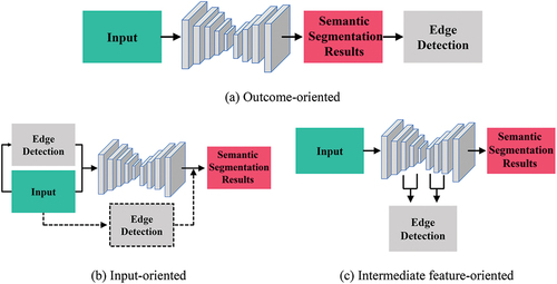
2. Input-oriented methods [Figure 1b] commonly input the edge detection result in following two manners. One is sequential (solid line). For instance, Marmanis et al. (2017) placed HED in front of the semantic segmentation network, and then concatenated its output as the input of the latter. Similarly, Xu et al. (2021) firstly captured the boundary of HRSI with a category boundary detection network, then utilized the extracted boundary and HRSI as inputs. The other is parallel (dotted line), such as EDN (Nong et al. 2021), ESNet (Lyu et al. 2019) and HED-PSPNet (Jiao, 2022), which employs semantic segmentation and edge detection subnetworks in parallel. These studies demonstrated that edge detection contributes to semantic segmentation. However, relative independence of the two tasks leads to high model complexity and weak feature coupling.

3. Intermediate feature-oriented methods [Figure 1c] share the hierarchical features of semantic segmentation and edge detection. Chen et al. (2016) put forward a progressive DeepLab to predict edge with the intermediate features, and then optimizes coarse predictions with domain transform. Yu et al. (2018) introduced a discriminative feature network (DFN) that involves a smooth subnetwork and a border subnetwork. In addition, edge detection tasks in ERN (Liu et al. 2018) and FusionNet (Cheng et al. 2017) were proved to be beneficial, however, they failed to employ extensive helpful intermediate features (Liu et al. 2018). Our proposed work also falls into this category. DFN, ERN and FusionNet merely refined network parameters by boundary constraint, and progressive DeepLab (Chen et al. 2016) refined both of the parameters and the output probability map, which are insufficient to utilize multilevel features. Differently, the proposed method utilized intermediate dense features of edge detection branch to enhance semantic segmentation.

Although DCNN-based semantic segmentation methods emerge rapidly and get exciting results, they have some shortcomings when dealing with complicated remote sensing images:

1. DCNN segmentation methods for natural images struggle to deal with complex features of HRSIs. The scale variance and feature complexity of HRSIs make ground objects indistinguishable (Du et al. 2020; Liu et al. 2017).

2. The semantic segmentation methods for HRSIs are hard to get ideal results because severe inter-class fuzziness and intra-class discrepancies, the boundary blur and incompleteness are common (Diakogiannis et al. 2020; Ding, Tang, and Bruzzone 2020; Li et al. 2021; Zuo et al. 2021).

3. Most semantic segmentation methods enhanced by edge detection are limited by insufficient feature integration and redundant feature extraction structure, resulting in relatively high model complexity and poor performance (Cheng et al. 2017; Jiao et al. 2022; Liu et al. 2018; Lyu et al. 2019; Marmanis et al. 2017; Nong et al. 2021; Xu, Su, and Zhang 2021; Yu et al. 2018).

Therefore, a novel boundary-enhanced dual-stream network (BEDSN) with one semantic segmentation branch stream (SSBS) and one edge detection branch stream (EDBS) is proposed to solve these shortcomings. In brief, it is a two-branch full-resolution network with various modules to enhance feature extraction and feature recovery abilities, while the post process can further refine the results. It takes the advantages of DCNN-based semantic segmentation, while EDBS effectively compensate for boundary loss. In brief, the primary contributions of BEDSN are presented as follows:

1. Highly coupled structure and effective reuse of intermediate boundary information. Compared with other methods (Cheng et al. 2017; Jiao et al. 2022; Liu et al. 2018; Lyu et al. 2019; Marmanis et al. 2017; Nong et al. 2021; Xu, Su, and Zhang 2021; Yu et al. 2018), the proposed method realizes stronger integration of semantic segmentation and edge detection, which is beneficial for keeping the integrity of edges, thus reducing semantic ambiguity and intra-class inconsistency.

2. Efficient feature extraction and utilization. Improved multiscale feature extraction module (MSFM) and hybrid atrous convolution module (HACM) are utilized to acquire multiscale contextual information. In addition, a channel attention-guided multilevel information fusion module (MIFM) is proposed to integrate intermediate features from EDBS and narrow semantic gaps. These structures efficiently extract the multiscale features and are effective when dealing with remote sensing images.

The rest of this article is organized as follows. The proposed BEDSN is introduced in Section 2. The results of experiments and discussions are reported in Section 3. Finally, the conclusions are drawn in Section 4.

2. Methodology

2.1. Overall architecture of BEDSN

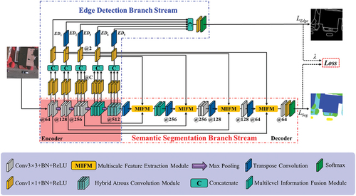
The details of BEDSN and how it benefits from edge detection is introduced in this section. As shown in Figure 2, BEDSN is composed of two branch streams, i.e. a progressive SSBS and a lightweight EDBS. SSBS is responsible for fine semantic segmentation, while EDBS realizes boundary feature supervision and refines the result of SSBS. Both streams can be learned end-to-end and optimized simultaneously. Their feature interconnection is realized by two means. (1) One lies in the encoder part where the features are mutual. The stronger interaction is realized by feature sharing, while the increased model parameters brought by EDBS are extremely negligible. (2) The other exploits boundary to guide feature extraction further in the decoder part of SSBS.

Figure 2. Overall architecture of the proposed BEDSN.

2.2. Semantic Segmentation Branch Stream (SSBS)

In this study, UNet serves as the baseline, and the architecture of SSBS is modified as follows. MSFM and HACM are integrated into SSBS to better distinguish multiscale objects. Transposed convolution improves the feature recovery and MIFM fuses features from SSBS and EDBS to promote the efficiency.

In general, SSBS is made up of two components: an encoder for spatial size reduction of feature maps and contextual information, and a decoder for resolution recovery and dense prediction. The encoder involves five stages. The first two stages contain two sub-blocks, while the third stage contains three sub-blocks. Every sub-block in the first three stages involves a 3 × 3 convolution layer followed by batch normalization (BN) and a rectified linear unit (ReLU) activation function. Three MSFMs are introduced in the fourth stage, and a HACM is employed in the fifth stage. Max-pooling (2 × 2) is performed after each stage (except the last one) for downsampling. Subcomponents in the decoder are nearly symmetric with those of the encoder. In addition, MIFM is used after upsampling to integrate both the detailed feature in encoder and boundary feature in EDBS into the decoder of SSBS. Details are presented in Figure 2, where @n represents the number of layers in the convolution.

2.3. Multiscale Feature Extraction Module (MSFM)

Multiscale contextual features of HRSIs are crucial to maintain semantic consistency inside the same object and strengthen the recognition of different objects. Convolution with relatively small receptive field, such as 1 × 1 or 3 × 3, will focus on small objects, resulting in fragmentation and inconsistency inside the large objects. By contrast, convolution with large respective field will be incapable of discriminating neighbor items (Zheng et al. 2019). To this end, lightweight MSFMs are applied in BEDSN to replace standard convolutions in the fourth stage of the encoder and corresponding layers of the decoder.

As shown in Figure 3, MSFM consists of four parallel convolution blocks with different kernel sizes of 1 × 1, 3 × 3, 5 × 5, and 7 × 7. Large convolution kernels can capture long-range contextual information but lead to expensive cost. Hence, a 1 × 1 convolution is utilized before 3 × 3, 5 × 5 and 7 × 7 convolutions for feature reduction (Lateef and Ruichek 2019). Meanwhile, the channel depth is set as Table 1. These parallel convolution blocks are then concatenated to acquire multiscale feature map.

Figure 3. Diagram of MSFM.

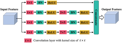
Table 1. Channel depth of each convolution block.

Layer ID	L1_1	L2_l	L2_2	L3_1	L3_2	L4_1	L4–2
Encoder	1×1,64	1×1,192	3×3,256	1×1,64	5×5,128	1×1,32	7×7,64
Decoder	1×1,64	1×1,256	3×3,128	1×1,64	5×5,32	1×1,32	7×7,32

Lm_n (m = 1, 2, 3, 4; n = 1, 2) denotes the convolutional layer n of the parallel branch m in MSFM.

2.4. Hybrid Atrous Convolution Module (HACM)

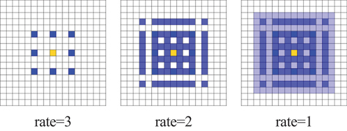
HACM is leveraged in the last stage of the encoder to capture richer contextual information and alleviate the contradiction between local details and global semantics (Chen et al. 2015; Zheng et al. 2021). HACM is designed with three successive atrous convolution layers. As illustrated in Figure 4, receptive field of three consecutive atrous convolutions with dilation rates of (Huang et al. 2021) can cover the entire square region and obtain a local receptive field with size of 13 × 13. With different dilation rates, the gridding problem can be eliminated (Wang et al. 2017).

Figure 4. Diagram of HACM. Coverage maps of local receptive field for the three atrous convolutions with different dilation rates are presented from left to right.

2.5. Transposed convolution layers

Unlike the original upsampling of UNet, BEDSN gradually restores the resolution by exploiting the transposed convolution (deconvolution) (Fergus, Taylor, and Zeiler 2011). The deconvolution with a stride of 2 and kernel size of 4 is utilized in BEDSN to eliminate checkerboard artifacts (Odena, Dumoulin, and Olah 2016). Moreover, deconvolutions can be applied as both upsampling operators and feature extractors, thus the number of sub-blocks in each stage of the decoder is reduced by one.

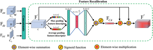
2.6. Multilevel Information Fusion Module (MIFM)

In SSBS, fine features from the encoder ($F_{\mathit{en}}$) and boundary features from EDBS ($F_{\mathit{ED}}$) are fused with coarse semantic features from the decoder ($F_{\mathit{de}}$) to acquire abundant information of spatial details and boundary. There exist semantic gaps among features among different levels (Huang et al. 2021), hence merging them in a naive manner such as concatenation or element-wise summation may ignore their discrepancies. Therefore, MIFM guided by channel attention (Woo et al. 2018) is proposed to merge features efficiently.

Figure 5 shows the two steps of MIFM. $F_{\mathit{en}}$, $F_{\mathit{de}}$ and $F_{\mathit{ED}}$ are concatenated along the channel dimension in the first step to obtain the elementary fusion feature $F^{\prime }$. $F^{\prime }$ is then recalibrated by the feature recalibration submodule (FRM) in the second step (dotted box). In FRM, the channel attention feature map $F_{\mathit{CA}}\in R^{1\times 1\times \mathit{C}}$ of $F^{\prime }$ is firstly generated, $F_{\mathit{CA}}$ values are then broadcast along the spatial dimension via element-wise multiplication. The multiplication result is finally connected with the raw $F^{\prime }$ via residual structure to minimize information flow loss and obtain the fusion feature $F^{\prime \prime }$. Specifically, during the generation of $F_{\mathit{CA}}$, FRM firstly adopts max-pooling and average-pooling to aggregate spatial information, then two generated context descriptors were fed into a shared two-layer perceptron followed by a sigmoid function to produce $F_{\mathit{CA}}$. The whole process of MIFM can be expressed as follows:

Figure 5. Diagram of MIFM.

(1) $F^{\prime }=\mathcal{\S }\left(F_{\mathit{en}},F_{\mathit{de}},F_{\mathit{ED}}\right)$(1)

(2) $F^{\prime }=\mathit{\sigma }\left(W_1\left(\mathit{h}\left(W_0\left(\mathit{Avgpool}\left(F^{\prime }\right)\right)\right)\right)+W_1\left(\mathit{h}\left(W_0\left(\mathit{Maxpool}\left(F^{\prime }\right)\right)\right)\right)\right)$(2)

(3) $F^{\prime \prime }=F^{\prime }\otimes F_{\mathit{CA}}+F^{\prime }$(3)

Where ${\mathcal{\S }}^{\cdot \cdot }$ stands for the concatenation operation; $W_0$ and $W_1$ represent the weights of the first and second layers in the shared perceptron, respectively; $\mathit{h}$ and $\mathit{\sigma }$ represent the ReLU and sigmoid function, respectively; and $\otimes$ denotes the element-wise multiplication.

2.7. Edge Detection Branch Stream (EDBS)

Inspired by RCF, EDBS is introduced into BEDSN as the second branch stream. Unlike other studies which only make use of features from some special layers (Cheng et al. 2017; Jin et al. 2023; Liu et al. 2018), EDBS exploits all convolutional features of the encoder. EDBS is shown in the blue dashed box of Figure 2. Each feature from the encoder is first fed to a 1 × 1 convolution, whose channel depth is equal to the number of semantic segmentation categories. The acquired feature is then concatenated with others from the same stage. A 1 × 1 × 2 convolution is implemented for information exchange. Thereafter, the boundary feature whose size is smaller than the input will be upsampled to the input size via transposed convolution, obtaining five boundary feature maps from different stages, namely, $\mathit{E}{D}_1$, $\mathit{E}{D}_2$, $\mathit{E}{D}_3$, $\mathit{E}{D}_4$, and $\mathit{E}{D}_5$. Finally, a 1 × 1 × 2 convolution and a softmax layer are applied after the concatenation of {$\mathit{E}{D}_1$, $\mathit{E}{D}_2$, $\mathit{E}{D}_3$, $\mathit{E}{D}_4$ and $\mathit{E}{D}_5$} to detect the edge.

EDBS optimizes the feature extractor by controlling gradient information, while intermediate features are gradually integrated into SSBS, the result of semantic segmentation is improved. As EDBS is well trained, the shared feature extractor is more capable of catching boundary information than a single SSBS, and MIFMs further optimize the decoder of SSBS. Therefore, semantic segmentation results with boundary refined are acquired by SSBS in predicting process only.

Intra-class heterogeneity and inter-class homogeneity are solved by not only the dual-stream architecture but the utilization of various modules. On the one hand, EDBS takes edge label into consideration, which is helpful for boundary information extraction, it has the advantage of distinguishing the accurate edge of different classes with similar spectrum. One the other hand, MSFM, HACM and MIFM enhance the ability of feature extraction and the fitting ability of semantic segmentation branches, thereby making it possible to regard heterogeneous category as a whole.

2.8. Joint loss function

As BEDSN is a combination of SSBS and EDBS, two different loss functions are employed separately in network training. The standard cross-entropy loss function is used by SSBS:

(4) $L_{\mathit{Seg}}=-\frac{1}{N}\sum _{\mathit{n}=1}^N\sum _{\mathit{c}=1}^C{l_c}^{\left(\mathit{n}\right)}log\left({p_c}^{\left(\mathit{n}\right)}\right)$(4)

where N denotes the total number of pixels, C represents the number of categories, ${l_c}^{\left(\mathit{n}\right)}$ is the true label of the sample n for class c under the one-hot encoding scheme, and ${p_c}^{\left(\mathit{n}\right)}$ is the softmax probability of sample n belonging to class c.

The following edge-sensitive binary cross-entropy loss function is introduced in EDBS:

(5) $L_{\mathit{ED}}=-\sum _{\mathit{n}=1}^N\left(\frac{1}{E^{+}}{y}^{\left(\mathit{n}\right)}log{\stackrel{\wedge }{\mathit{y}}}^{\left(\mathit{n}\right)}+\frac{1}{E^{-}}\left(1-y^{\left(\mathit{n}\right)}\right)log\left(1-{\stackrel{\wedge }{\mathit{y}}}^{\left(\mathit{n}\right)}\right)\right)$(5)

where $E^{+}$ and $E^{-}$ represent the number of pixels located in boundary and nonboundary areas, respectively; $y^{\left(\mathit{n}\right)}\left(\in \left\{0,1\right\}\right)$ is the true label of sample n; $y^{\left(\mathit{n}\right)}=1$ means it is a boundary pixel and $y^{\left(\mathit{n}\right)}=0$ means it is a nonboundary pixel; and represents the probability that sample n is a boundary pixel. Accordingly, $L_{\mathit{ED}}$ can be regarded as the sum of average losses of boundary and nonboundary regions, thereby imposing a larger penalty to boundary loss.

Hence, the total joint loss function is defined as follows:

(6) $\mathit{Loss}=L_{\mathit{Seg}}+\mathit{\lambda }{L}_{\mathit{ED}}$(6)

where the hyperparameter $\mathit{\lambda }$ is used to balance EDBS and SSBS.

3. Experiments details

Based on experimental datasets, the comparison and ablation experiments were conducted, respectively, to assess the proposed method. Meanwhile, studies on training parameters, loss functions and model arrangement were discussed to verify the reasonableness of BEDSN and the experiments.

3.1. Datasets

The Vaihingen and Potsdam datasets (2018) were used to evaluate the performance. They are both aerial imagery datasets consisting of true orthophoto maps (TOP), ground truth labels (GT), and digital surface models (DSMs). Each dataset is categorized into six classes, including building, impervious surfaces, low vegetation, tree, car, and clutter/background. Data distributions are illustrated in Figure 6.

Figure 6. Experimental data distribution maps.

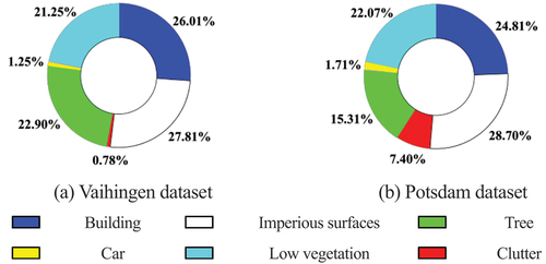
The Vaihingen dataset is composed of 33 patches with different sizes ranging from 1281 × 2336 to 2550 × 3816, and its resolution is 9 cm. TOPs consist of three bands, namely, near infrared (IR), red (R), and green (G) bands. All experiments were conducted without DSMs. Furthermore, similar to previous studies (Zheng et al. 2021), this work utilized 16 patches for training and another 17 patches for testing.

The Potsdam dataset comprises 38 patches with the same size (6000 × 6000) and resolution of 5 cm. Different from the Vaihingen dataset, TOPs with two more channel compositions (R-G-B and R-G-B-IR) along with the normalized DSMs (nDSMs) are provided in addition to IR-R-G TOPs and DSMs. However, Only R-G-B TOPs were introduced during both training and testing. Furthermore, similar to previous studies (Zheng et al. 2021), 24 patches were chosen for training while the remaining 14 patches were used for assessment.

3.2. Implementation details

All experiments were implemented by TensorFlow framework. Moreover, the experiments on the Vaihingen dataset were conducted with NVIDIA GeForce RTX 2080Ti GPU, while experiments on the Potsdam dataset were executed with NVIDIA Quadro RTX 5000 GPU.

3.2.1. Training phase

Data augmentation was performed, including random cropping, horizontal and vertical flipping, and rotating at intervals of 90°. A total of 16,000 and 24,000 training samples with the size of 256 × 256 were yielded for Vaihingen and Potsdam datasets, respectively. The reference boundary labels used for the supervised training of EDBS were obtained from GT of semantic labels. Specifically, if one pixel is different from its four neighbors, then it will be viewed as a boundary pixel. For fairness, all networks were trained from scratch and the training epochs were 60. Network training is executed with the adaptive moment estimation (ADAM) optimizer, and the initial learning rate is 3 × 10⁻⁴.

3.2.2. Test phase

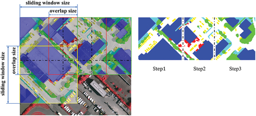
Overlap clipping inference strategy was adopted owing to the limitation of GPU memory. As depicted in Figure 7, a sliding window was used to traverse the test image, then the semantic segmentation results of cropped images could be stitched together. Concretely, two sliding windows overlap each other, and half of the results of the overlapped area were obtained by the front window while the other half was derived by the rear window, given that the predictions in central area of each patch is more accurate than those near the boundary. Besides, the ensemble learning was introduced during test to improve the generalizability.

Figure 7. Diagram of overlap clipping inference. Only the first horizontal traversal is presented for better visual effects.

3.3. Evaluation metric

Three kinds of evaluation metrics were adopted to assess different methods. One focuses on the accuracy of semantic segmentation results, including overall accuracy (OA), Kappa coefficients (Kappa), average F1 score (AF), and mean intersection over union (MIoU). AF and MIoU are calculated by averaging all F1 scores and IoUs of each class. They are defined as follows:

(7) $\mathit{OA}=\frac{\mathit{TP}+\mathit{TN}}{\mathit{TP}+\mathit{TN}+\mathit{FP}+\mathit{FN}}$(7)

(8) $\mathit{Kappa}=\frac{\mathit{N}\sum _{\mathit{k}=1}^C{n}_{\mathit{kk}}-\sum _{\mathit{k}=1}^C{n}_{\mathit{k}+}{n}_{+\mathit{k}}}{N^2\underset{\mathit{k}=1}{\overset{C}{-\sum }}{n}_{\mathit{k}+}{n}_{+\mathit{k}}}$(8)

(9) $F_1=\frac{2\mathit{TP}}{2\mathit{TP}+\mathit{FP}+\mathit{FN}}$(9)

(10) $\mathit{IoU}=\frac{\mathit{TP}}{\mathit{TP}+\mathit{FP}+\mathit{FN}}$(10)

where TP, FP, TN, and FN represent true positive, false positive, true negative, and false negative, respectively; N is the total number of pixels in test images; C is the number of categories; $n_{\mathit{k}+}$ and $n_{+\mathit{k}}$ correspond to the number of pixels belonging to class k and predicted to class k, respectively.

Another kind of metrics focuses on boundary blur, it compares the boundary of predictions and true boundary labels by a binary classification-based method, given that the edge results are composed of boundary and nonboundary pixels. Usually, the boundary of true labels is of good consistency and the boundary of predictions is relatively unstable, dilation of binary images was utilized for true boundary labels. The formula of boundary blur can be expressed as:

(11) $\begin{array}{c}\mathrm{Ac}{\mathrm{c}}_{\mathit{edge}}=\mathit{F}\left(\mathit{recall}\left(\mathit{Dilatio}{n}^n\left(\mathit{Edg}{e}_{\mathit{GT}}\right),\mathit{Edg}{e}_{\mathit{predict}}\right),\left(\mathit{Dilatio}{n}^n\left(\mathit{Edg}{e}_{\mathit{GT}}\right),\mathit{Edg}{e}_{\mathit{predict}}\right)\right)\end{array}$(11)

where Edge denotes the boundary label of ground truth or prediction,$\mathit{Dilatio}{\mathit{n}}^{\mathit{n}}$ represents dilation with the kernel size of n and F is a function.

The last kind of metric is model complexity, which assesses the number of trainable parameters and the number of floating-point operations (FLOPs) (He and Sun, 2015; Molchanov et al. 2016), respectively.

3.4. Experiment design

In order to validate the effectiveness of the proposed BEDSN, eleven state-of-the-art models were carried out on both datasets as comparison, including FCN-8s (Long, Shelhamer, and Trevor 2017), UNet (Ronneberger, Fischer, and Brox 2015), SegNet (Badrinarayanan, Kendall, and Cipolla 2017), PSPNet (Zhao et al. 2017), DeepLabv3+ (Chen et al. 2018), ERN (Liu et al. 2018), ResUNet-a (Diakogiannis et al. 2020), SCAttNet (Li et al. 2021), GAMNet (Zheng et al. 2021), LANet (Ding, Tang, and Bruzzone 2020) and MDANet (Zuo et al. 2021). Furthermore, for PSPNet, DeepLabv3+, and GAMNet, ResNet-101 (He et al. 2016) was selected as the feature extractor; for ResUNet-a, the basic version without multitask inferencing was chosen; for SCAttNet, the version with SegNet as the backbone was implemented; and for LANet, the version with embeded low-level features was utilized. Besides, the comparison on boundary blur were discussed on both datasets.

When it comes to model architecture, ablation experiments on different network modules and arrangement of dual streams were studied. Meanwhile, to make an exhaustive study of the proposed BEDSN, the influence of loss function, training parameters was discussed.

4. Results and discussion

4.1. Comparison experiments and analysis

4.1.1. Comparison on semantic segmentation

Quantitative analysis (Vaihingen dataset). Table 2 reports the evaluation of different methods on the Vaihingen dataset. As shown in Figure 6a, the clutter/background only occupies a tiny ratio in Vaihingen, thus this class is excluded which is similar to (Z. Zheng et al. 2021) and (Zhang et al. 2020). The results showed that the proposed BEDSN is the best in terms of overall performance among all the twelve methods. Compared with the baseline UNet, BEDSN performs better while saving approximately 31.48% of parameters and 23.25% of FLOPs. Moreover, BEDSN improves the indicators of each category. BEDSN can also enhance the classification of intricate objects, F1 scores of low vegetation and tree increase by 2.54% and 1.33%, while IoUs increase by 3.69% and 2.12%, respectively. It can be concluded that: (1) BEDSN ranks first in performance with less parameters than other methods except ERN, (2) ERN performs better than some heavyweight methods with the least parameters (<7 million), (3) GAMNet shows highly limited performance with huge computational burden and memory. (4) LANet and MDANet are light-weight methods with low time cost, but their performance in accuracy is limited.

Table 2. Results of different methods on Vaihingen dataset.

Methods	Building	Imp-suf	Low-veg	Tree	Car	OA	Kappa	AF	MIoU	Parameters	GFLOPs	Test time
FCN-8s	87.46/77.71	86.13/75.64	75.44/60.57	85.33/74.41	73.53/58.15	83.69	78.36	81.58	69.30	136.83M	57.29	9.13s
UNet	93.88/88.46	91.41/84.18	81.17/68.30	87.91/78.44	84.45/73.08	88.83	85.19	87.76	78.49	31.04M	109.31	15.36s
SegNet	92.77/86.52	90.05/81.90	80.08/66.78	87.32/77.50	69.97/53.81	87.65	83.62	84.04	73.30	29.46M	81.41	11.09s
PSPNet	92.37/85.83	90.44/82.56	81.47/68.73	88.39/79.20	70.35/54.47	88.20	84.34	84.64	74.16	46.71M	46.15	15.35s
DeepLabv3+	93.55/87.87	91.05/83.57	81.40/68.64	88.03/78.62	80.46/67.30	88.71	85.03	86.90	77.20	59.37M	146.70	10.89s
ERN	93.77/88.27	91.02/83.52	81.33/68.54	87.93/78.45	85.34/74.43	88.76	85.09	87.88	78.64	6.63M	57.57	12.49s
SCAttNet	92.14/88.27	89.62/83.52	81.65/69.00	88.30/79.05	74.42/59.26	87.85	83.88	85.23	74.78	29.46M	82.67	11.10s
ResUNet-a	93.02/86.95	89.56/81.09	81.77/69.16	88.00/78.57	77.08/62.70	88.53	84.79	86.21	76.23	48.77M	93.29	16.46s
GAMNet	91.20/83.82	89.56/81.09	78.88/65.13	87.30/77.47	79.01/65.30	86.88	82.61	85.19	74.56	387.4M	245.23	19.83s
LANet	90.67/82.93	89.31/80.68	78.15/64.14	87.09/77.13	80.86/67.87	87.03	82.08	85.22	74.55	23.79M	8.29	3.71s
MDANet	91.27/83.94	89.46/80.92	78.35/64.40	87.26/77.39	80.82/67.82	87.33	82.46	85.43	74.90	31.90M	11.06	8.89s
BEDSN	94.71/89.95	92.30/85.71	83.71/71.99	89.24/80.56	86.31/75.92	90.14	86.93	89.25	80.82	21.27M	83.89	15.53s

For brevity, Imp-surf and Low-veg denote the impervious surface and the low vegetation classes, respectively. Note that evaluations for per class are presented in the form of F1%)/IoU (%), optimal values are presented in bold font, and suboptimal values are presented in blue font. The test time is calculated on the basis of area 10 of Vaihingen dataset.

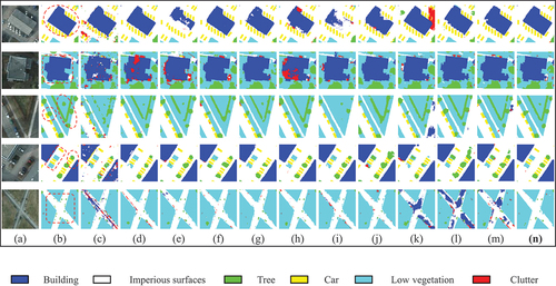
Visualization analysis (Vaihingen dataset). The results for complete tiles of the Vaihingen dataset are shown in Figure 8. Meanwhile, the results of local areas are presented in Figure 9. BEDSN presents superior performance in the following aspects:

Figure 8. Results for complete tiles of the Vaihingen dataset: areas 27 (top) and 31(bottom). (a) original, (b) GT, (c) FCN–8s, (d) UNet, (e) SegNet, (f) PSPNet, (g) DeepLabv3+, (h) ERN, (i) SCAttNet, (j) ResUNet-a, (k) GAMNet, (l) LANet, (m) MDANet, (n) proposed BEDSN.

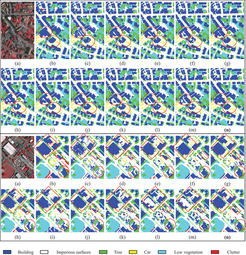
Figure 9. Results for local areas of the Vaihingen dataset. (a) original, (b) GT, (c) FCN–8s, (d) UNet, (e) SegNet, (f) PSPNet, (g) DeepLabv3+, (h) ERN, (i) SCAttNet, (j) ResUNet–a, (k) GAMNet, (l) LANet, (m) MDANet, (n) proposed BEDSN.

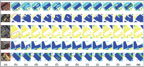
Intra-class consistency. BEDSN is more effective in reducing the influence of inter-class similarity and exhibits better intra-class consistency. As circled in Figure 8, in terms of buildings, BEDSN can successfully regard them as a whole, DeepLabv3+ generates suboptimal results, while other methods tend to predict part of buildings as impervious surfaces. Figure 9 also confirms such superiority of BEDSN. Moreover, when confronted with shadows, BEDSN is still competent to produce relatively complete results while other methods usually lead to misclassification.

Accurate contour. BEDSN shows excellent performance in capturing more precise contours, especially for densely distributed buildings and cars with evident boundaries. As shown in all the tagged areas in both Figures 8 and 9, BEDSN can preserve more boundary features, prompting clearer corners and boundaries than other methods.

Quantitative analysis (Potsdam dataset). The numerical results of the Potsdam dataset are listed in Table 3. The clutter/background class is considered because it accounts for a relatively large proportion (right block of Figure 6). According to Table 3, the proposed BEDSN achieves optimal performance. Similar to the Vaihingen dataset, the Potsdam dataset also demonstrates significant improvements.

Table 3. Results of different methods on Potsdam dataset.

Methods	Building	Imp-suf	Low-veg	Tree	Car	Clutter	OA	Kappa	AF	MIoU
FCN-8s	84.78/73.58	83.28/71.35	78.78/64.99	77.62/63.43	87.38/77.59	27.80/16.14	79.13	72.81	73.27	61.18
UNet	93.82/88.35	90.14/82.05	84.22/72.74	85.65/74.90	93.02/86.95	35.69/21.72	86.91	82.86	80.42	71.12
SegNet	94.93/90.34	91.44/84.22	85.26/74.30	86.82/76.72	94.46/89.50	47.10/30.80	88.45	84.88	83.33	74.32
PSPNet	92.53/86.10	90.10/81.98	83.77/72.07	83.53/71.71	93.43/87.66	40.25/25.20	86.24	81.96	80.60	70.79
DeepLabv3+	94.65/89.85	90.63/82.87	83.76/72.06	83.55/71.43	93.53/87.84	40.26/25.20	87.48	83.51	81.03	71.54
ERN	93.44/87.69	89.82/81.52	84.23/72.76	83.33/75.41	93.53/88.13	34.95/21.18	86.46	82.31	80.32	71.07
SCAttNet	95.26/90.96	91.26/83.93	83.79/72.10	85.12/74.10	92.66/86.32	46.63/30.41	88.00	84.26	82.46	72.97
ResUNet-a	92.86/86.68	89.00/80.19	83.00/70.95	82.28/69.89	91.73/84.72	36.20/22.10	85.84	81.37	79.18	69.09
GAMNet	92.41/85.89	87.11/77.16	79.60/66.12	80.53/67.40	93.04/86.99	30.02/17.66	83.22	78.14	77.12	66.87
LANet	92.68/86.36	88.90/80.02	81.50/68.78	83.64/71.88	94.62/89.79	34.77/21.04	85.37	80.85	79.35	69.65
MDANet	92.86/86.67	89.11/80.35	81.42/68.67	83.86/72.20	94.57/89.69	33.96/20.45	85.55	81.08	79.29	69.67
BEDSN	95.64/91.64	91.83/84.90	85.85/75.20	86.72/76.55	95.03/90.53	49.42/32.82	89.17	85.78	84.08	75.27

For brevity, Imp-surf and Low-veg denote the impervious surface and the low vegetation classes, respectively. Note that evaluations for per class are presented in the form of F1%)/IoU (%), optimal values are presented in bold font, and suboptimal values are presented in blue font.

Visual analysis (Potsdam dataset). Figure 10 shows the results of the Potsdam dataset. Figure 11 displays more detailed results. The performance of the proposed BEDSN on the Potsdam dataset is consistent with that on the Vaihingen dataset. (a) BEDSN generates more accurate results. For instance, the marked areas of Figures 10 and 11 demonstrate that building interiors predicted by BEDSN are more complete. (b) BEDSN performs well in capturing sharp boundaries such as corners of buildings, and the prediction of impervious surfaces is comparatively exact. To sum up, the results of Vaihingen dataset and Potsdam dataset exhibit the accuracy and robustness of BEDSN quantitatively and visually.

Figure 10. Results for complete tiles of the Potsdam dataset: areas 5_13 (top) and 5_14 (bottom). (a) original, (b) GT, (c) FCN–8s, (d) UNet, (e) SegNet, (f) PSPNet, (g) DeepLabv3+, (h) ERN, (i) SCAttNet, (j) ResUNet–a, (k) GAMNet, (l) LANet, (m) MDANet, (n) proposed BEDSN.

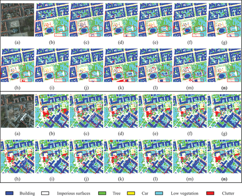
Figure 11. Results of local areas on the Potsdam dataset. (a) original, (b) GT, (c) FCN–8s, (d) UNet, (e) SegNet, (f) PSPNet, (g) DeepLabv3+, (h) ERN, (i) SCAttNet, (j) ResUNet–a, (k) GAMNet, (l) LANet, (m) MDANet, (n) proposed BEDSN.

4.2. Comparison on boundary blur

In order to make a comprehensive study of boundary blur, the edge of ground truth labels and predictions were considered. After edge extraction and morphological dilation, the ground truth edge labels serve as the basis, and recall, precision and F1 score were calculated to measure the similarity between edge of predictions and the basis. It is worthwhile that TP, FP, FN and TN in Tables 4–5 denote the total pixel numbers, the visual results of boundary blur are shown in Figure 12. As shown in Tables 4–5, BEDSN has the highest precision and F1 score among all methods, while the recall is slightly lower than the best method, it indicates that a large portion of predicted boundary pixels of BEDSN is correct. Meanwhile, the performance in respect of precision and F1 score is improved by 1.76%, 0.80% for Vaihingen dataset and 3.25%, 0.88% for Potsdam dataset respectively.

Figure 12. Results of boundary blur on the Potsdam dataset: a part of area 7_13 (a patch identification number of Potsdam dataset). (a) original, (b) GT, (c) edge, (d) dilated edge, (e) FCN–8s, (f) UNet, (g) SegNet, (h) PSPNet, (i) DeepLabv3+, (j) ERN, (k) SCAttNet, (l) ResUNet–a, (m) GAMNet, (n) LANet, (o) MDANet, (p) proposed BEDSN.

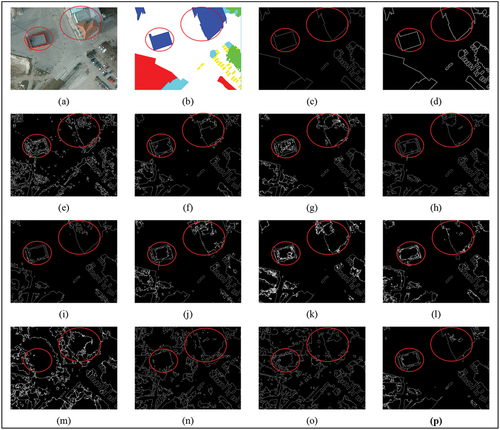
Table 4. Results of boundary metrics on Vaihingen dataset with dilated edge labels.

Methods	TP	FP	FN	TN	recall	precision	F1 score
FCN-8s	1376326	4159010	5459587	79205142	20.13%	24.86%	22.25%
UNet	1316870	1991482	5519043	81372670	19.26%	39.80%	25.96%
SegNet	1216539	2583025	5619374	80781127	17.80%	32.02%	22.88%
PSPNet	1075445	2190203	5760468	81173949	15.73%	32.93%	21.29%
DeepLabv3+	1253405	2164946	5582508	81199206	18.34%	36.67%	24.45%
ERN	1407411	2451553	5428502	80912599	20.59%	36.47%	26.32%
SCAttNet	1198432	2373216	5637481	80990936	17.53%	33.55%	23.03%
ResUNet-a	1246352	2347454	5589561	81016698	18.23%	34.68%	23.90%
GAMNet	1307215	2501804	5528698	80862348	19.12%	34.32%	24.56%
LANet	1283609	2229294	5552304	81134858	18.78%	36.54%	24.81%
MDANet	1280607	2142706	5555306	81221446	18.73%	37.41%	24.96%
BEDSN	1375792	1934438	5460121	81429714	20.13%	41.56%	27.12%

Table 5. Results of boundary metrics on Potsdam dataset with dilated edge labels.

Methods	TP	FP	FN	TN	recall	precision	F1 score
FCN-8s	5224168	28939699	19742606	450093527	20.92%	15.29%	17.67%
UNet	4599604	10052678	20367170	468980548	18.42%	31.39%	23.22%
SegNet	4918198	11396487	20048576	467636739	19.70%	30.15%	23.83%
PSPNet	3671640	9467582	21295134	469565644	14.71%	27.94%	19.27%
DeepLabv3+	3904419	8563245	21062355	470469981	15.64%	31.32%	20.86%
ERN	5031544	12841064	19935230	466192162	20.15%	28.15%	23.49%
SCAttNet	4881454	18016908	20085320	461016318	19.55%	21.32%	20.40%
ResUNet-a	4744242	18556613	20222532	460476613	19.00%	20.36%	19.66%
GAMNet	4926969	15746290	20039805	463286936	19.73%	23.83%	21.59%
LANet	4353693	9980000	20613081	469053226	17.44%	30.37%	22.16%
MDANet	4356780	9321809	20609994	469711417	17.45%	31.85%	22.55%
BEDSN	4759754	8799015	20207020	470234211	19.06%	35.10%	24.71%

The visualization results of different methods are depicted in Figure 12, as can be seen, the results of BEDSN, UNet, PSPNet and DeepLabv3+ are of good intra-class consistency, while BEDSN performs best. Furthermore, the boundary pixels of BEDSN are closest to ground truth edge, especially in the red circle areas, which further exhibits the excellent performance of BEDSN to solve intra-class inconsistency and boundary blur. It is obvious that the proposed BEDSN has the best ability to preserve boundary visually and statistically.

4.3. Ablation experiments and model arrangement

4.3.1. Ablation experiments

As introduced in Section 3, the proposed BEDSN is improved by EDBS and SSBS. The ablation experiments were accomplished by means of expanding the model architecture, such as uniting the edge detection task in feature-sharing manner, enhancing SSBS by HACM, transposed convolution, MIFM, and MSFM. The Vaihingen dataset was chosen as example.

The results are listed in Table 6. For convenience, intermediate models are called as Net1–Net5. It can be observed that all the strategies are conducive to reinforcing the performance. With the inclusion of depth dimension expansion, the performance in respect of OA, Kappa, AF, and MIoU is improved by 0.22%, 0.30%, 0.43%, and 0.66%, respectively. The performance is significantly reinforced at minimal cost when combined with edge detection, as model parameters and FLOPs increase by approximately 0.1% and 0.4% respectively. With the help of HACM, model parameters reduce significantly and OA improves slightly. By learning related parameters and improving the ability to recover detailed features, the transposed convolution is particularly useful for building and car classes. Besides, MIFM can enhance the discrimination ability for ground objects that are easily confused, such as impervious surface and tree classes. Finally, with MSFM, BEDSN demonstrates excellent performance in distinguishing impervious surface and tree classes. Moreover, MSFM encodes multiscale contextual information at low computational cost.

Table 6. Results of ablation experiments on Vaihingen dataset.

Methods	A	B	C	D	E	F	Building	Imp-suf	Low-veg	Tree	Car	OA	Kappa	AF	MIoU	Parameters	GFLOPs
UNet							93.88/88.46	91.41/84.18	81.17/68.30	87.91/78.44	84.45/73.08	88.83	85.19	87.76	78.49	31.04M	109.31
Net1	√						94.00/88.68	91.63/84.55	81.54/68.83	88.02/78.60	85.79/75.10	89.05	85.49	88.19	79.15	46.39M	133.47
Net2	√	√					94.26/89.14	91.83/84.90	82.51/70.23	88.52/79.41	86.11/75.60	89.48	86.06	88.65	79.86	46.44M	133.97
Net3	√	√	√				94.25/89.11	92.04/85.26	82.40/70.07	88.61/79.54	86.93/76.89	89.55	86.16	88.85	80.18	27.56M	112.41
Net4	√	√	√	√			94.62/89.80	92.01/85.36	82.47/70.17	88.59/79.52	87.07/77.10	89.71	86.36	88.97	80.39	30.94M	104.35
Net5	√	√	√	√	√		94.61/89.77	91.95/85.10	83.61/71.84	89.04/80.24	87.13/77.19	89.88	86.58	89.27	80.83	31.29M	104.40
BEDSN	√	√	√	√	√	√	94.71/89.95	92.30/85.71	83.71/71.99	89.24/80.56	86.31/75.92	90.14	86.93	89.25	80.82	21.27M	83.89

Note: “A,” “B,” and “C” denote depth dimension expansion, edge detection branch stream, and hybrid atrous block, respectively; while “D,” “E,” and “F” represent deconvolution, MIFM, and MSFM, respectively. Prominent positive and negative effects are presented in green and red fonts, respectively. Note that evaluations for per class are presented in the form of F1%)/IoU (%).

4.3.2. Arrangement of SSBS, EDBS and model efficiency

To evaluate the effects of SSBS and EDBS, SSBS was introduced to UNet to conduct experiments on both Vaihingen and Potsdam datasets. The numerical results are listed above the blue underscores of Table 7, and the visual results in Figure 13 demonstrate that both SSBS and EDBS can improve the performance. Model parameters and computation complexity are reduced by 31.57% and 23.69%, respectively, with SSBS introduced. Compared with UNet visually, SSBS enhances the ability to distinguish similar ground objects. The model is further enhanced with negligible costs when EDBS is integrated. Visually, EDBS guarantees precise boundary and enhanced intra-class consistency.

Figure 13. Results for the improved effects of SSBS and EDBS on Vaihingen (top) and Potsdam (below) datasets. (a) Image, (b) GT, (c) UNet, (d) SSBS, (e) BEDSN-P, (f) BEDSN, (g) Boundary results of BEDSN.

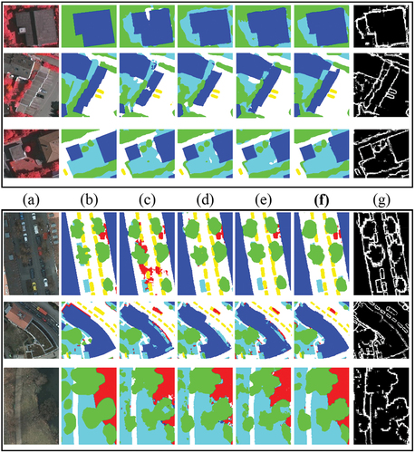
Table 7. Experiments on arrangement of SSBS, EDBS and efficiency.

Vaihingen Dataset

Methods

Building

Imp-suf

Low-veg

Tree

Car

Clutter

OA

Kappa

AF

MIoU

Parameters

GFLOPs

UNet

93.88/88.46

91.41/84.18

81.17/68.30

87.91/78.44

84.45/73.08

–

88.83

85.19

87.76

78.49

31.04M

109.31

PSPNet

92.37/85.83

90.44/82.56

81.47/68.73

88.39/79.20

70.35/54.47

–

88.2

84.34

84.64

74.16

46.71M

46.15

ERN

93.77/88.27

91.02/83.52

81.33/68.54

87.93/78.45

85.34/74.43

–

88.76

85.09

87.88

78.64

6.63M

57.57

LANet

90.67/82.93

89.31/80.68

78.15/64.14

87.09/77.13

80.86/67.87

–

87.03

82.08

85.22

74.55

23.79M

8.29

MDANet

91.27/83.94

89.46/80.92

78.35/64.40

87.26/77.39

80.82/67.82

–

87.33

82.46

85.43

74.90

31.90M

11.06

BEDSN

94.71/89.95

92.30/85.71

83.71/71.99

89.24/80.56

86.31/75.92

–

90.14

86.93

89.25

80.82

21.27M

83.89

SSBS

94.39/89.37

91.77/84.80

83.30/71.38

88.78/79.82

85.97/75.39

–

89.62

86.23

88.84

80.15

21.24M

83.41

BEDSN-P

94.28/89.18

91.77/84.80

83.07/71.04

88.91/80.02

86.41/76.97

–

89.63

86.24

89.00

80.40

32.79M

113.81

LBEDSN

94.45/89.47

91.72/84.71

83.36/71.46

88.99/80.16

85.12/74.10

–

89.67

86.31

88.73

79.98

5.33M

21.21

Potsdam Dataset

Methods

Building

Imp-suf

Low-veg

Tree

Car

Clutter

OA

Kappa

AF

MIoU

Parameters

GFLOPs

UNet

93.82/88.35

90.14/82.05

84.22/72.74

85.65/74.90

93.02/86.95

35.69/21.72

86.91

82.86

80.42

71.12

31.04M

109.31

PSPNet

92.53/86.10

90.10/81.98

83.77/72.07

83.53/71.71

93.43/87.66

40.25/25.2o

86.24

81.96

80.60

70.79

46.71M

46.15

ERN

93.44/87.69

89.82/81.52

84.23/72.76

83.33/75.41

93.53/88.13

34.95/21.18

86.46

82.31

80.32

71.07

6.63M

57.57

LANet

92.68/86.36

88.90/80.02

81.50/68.78

83.64/71.88

94.62/89.79

34.77/21.04

85.37

80.85

79.35

69.65

23.79M

8.29

MDANet

92.86/86.67

89.11/80.35

81.42/68.67

83.86/72.20

94.57/89.69

33.96/20.45

85.55

81.08

79.29

69.67

31.90M

11.06

BEDSN

95.64/91.64

91.83/84.90

85.85/75.20

86.72/76.55

95.03/90.53

49.42/32.82

89.17

85.78

84.08

75.27

21.27M

83.89

SSBS

95.24/90.91

91.05/83.56

85.38/74.49

86.13/75.63

94.43/89.45

42.31/26.83

88.49

84.85

82.42

73.48

21.24M

83.41

BEDSN-P

94.99/90.45

90.86/83.26

85.11/74.08

86.39/76.05

94.26/89.15

42.24/26.77

89.17

84.60

82.31

73.29

32.79M

113.81

LBEDSN

94.94/90.36

91.09/83.64

84.91/73.78

86.16/75.69

93.45/87.71

43.43/27.75

88.17

84.47

82.33

73.16

5.33M

21.21

As said in Section 3, the feature-sharing strategy was applied to arrange SSBS and EDBS. To check its effectiveness, this part employs a parallel mode of SSBS and EDBS named BEDSN-P, in which the encoders are independent but identical.

The results of BEDSN-P on two datasets are presented in Table 7. It is obvious that feature-sharing fashion of SSBS and EDBS is better than parallel fashion. Compared with SSBS, BEDSN-P shows a weak improvement when increasing nearly half of model parameters and calculation complexity. It reveals that the manner of feature-sharing can achieve strong information coupling and extract more meaningful features. Whereas, information coupling in the parallel arrangement is relatively weak and focuses more on EDBS, thereby leading to information degradation.

Besides, to explore the efficiency of BEDSN, this work simplifies it by deleting half of the filters in each layer of SSBS. The generated light-weight model (named LBEDSN) contains less parameters than ERN and lower computational cost than PSPNet whose FLOPs is the optimal among all the comparison methods described in Section IV except LANet and MDANet, while the LANet and MDANet struggle to get ideal result. The corresponding comparison results on both datasets are also presented in Table 7. It confirms the superiority of the proposed BEDSN, given that LBEDSN significantly outperforms UNet, ERN, and PSPNet with minimum model parameters and computational complexity.

4.4. Effect of joint loss function and training parameters

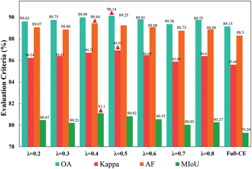
A comparison experiment with full cross-entropy loss function (Full-CE) was conducted to examine the performance of the joint loss function defined in Equation (6)(6) $\mathit{Loss}=L_{\mathit{Seg}}+\mathit{\lambda }{L}_{\mathit{ED}}$(6) . The experiments on λ ranging from 0.2 to 0.8 with the interval of 0.1 were carried out. Note that all experiments are based on the Vaihingen dataset and BEDSN. Figure 14 indicates that for the joint loss function, λ = 0.5 yields the optimal OA and Kappa, while AF and MIoU reach the optimum when λ = 0.4. It can be found that the Full-CE loss function is far inferior to the joint loss function, which indicates that edge information, also known as gradient information, does have positive impact on semantic segmentation. In a word, a small λ means insufficient boundary feature and limited supplementary information, which struggles to reach an ideal result. Meanwhile, too large weight for edge detection loss emphasizes too much on edge detection branch, thus makes semantic segmentation become relatively secondary task.

Figure 14. Semantic segmentation results of different λ and loss functions. Optimal indicators are marked with red triangles.

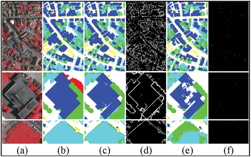
Examples of the visual results are shown in Figure 15. The results manifest that the edge detection predictions of the Full-CE are fragmented. Differently, the joint loss function can capture accurate contours, owing to the restrictions on category consistency.

Figure 15. Results of the joint loss function and Full–CE. (a) Image, (b) GT, (c)–(d) Segmentation and boundary predictions of the joint loss function (λ = 0.5), (e)–(f) Segmentation and boundary predictions of Full–CE.

In order to verify the impact of training parameters and find out the optimal parameters of BEDSN, comparative experiments of learning rate and batchsize were conducted on Vaihingen dataset with the help of Nvidia Quadro RTX5000. The batchsize were set to 2, 4, 8 and 12 while the learning rate were set from 3 × 10⁻⁵ to 0.3 with 10 as ratio. The results were shown in Table 8 and Table 9. Note that the metrics of each category are in the form of F1/IoU from Table 8 to Table 9.

Table 8. Experiments on different batchsizes with learning rate of 3 × 10⁻⁴.

Batchsize	Building	Imp-suf	Low-veg	Tree	Car	OA	Kappa	AF	MIoU
2	–/–	–/–	–/–	–/–	–/–	–	–	–	–
4	94.67/89.88	91.82/84.88	83.32/71.41	89.14/80.41	86.72/76.55	90.47	86.55	89.13	80.63
8	94.70/89.93	91.94/85.08	83.93/72.31	89.17/80.45	87.89/78.39	90.59	86.75	89.52	81.23
12	94.75/90.02	92.18/85.49	83.59/71.80	89.10/80.34	87.08/77.12	90.59	86.72	89.34	80.95

Table 9. Experiments on different learning rates with the batchsize of 8.

Learning rate	Building	Imp-suf	Low-veg	Tree	Car	OA	Kappa	AF	MIoU
0.3	92.97/86.86	89.93/81.70	79.20/65.57	87.75/78.17	78.94/65.20	88.22	83.73	85.76	75.50
0.03	94.62/89.79	92.36/85.80	81.57/68.88	88.11/78.74	86.63/76.42	89.90	86.06	88.66	79.93
0.003	94.62/89.79	92.14/85.42	82.79/70.63	88.74/79.76	86.19/75.73	90.19	86.54	88.90	80.27
0.0003	94.70/89.93	91.94/85.08	83.93/72.31	89.17/80.45	87.89/78.39	90.59	86.75	89.52	81.23
0.00003	93.51/87.81	90.62/82.86	81.54/68.84	88.10/78.74	82.75/70.57	89.17	84.80	87.30	77.76

As can been seen in Table 8, with the increase of batchsize, the four indexes increase slightly and the training time per epoch is reduced to some extent. The training process with batchsize of 2 had something wrong and the calculation of edge loss resulted in not a number (nan), leading to a low accuracy. As batchsize increased, the data distribution per batch became stable thus leading to the sound optimization of networks, this trend is significant while the batchsize is not so big. Therefore, it is crucial to maximize the batchsize while the accuracy can be improved and the memory of device is adequate. Notably, RTX2080Ti GPU served as the device of previous experiments and the maximum batchsize of Vaihingen dataset was set to 8, so the metrics in Table 8 are slightly better than those of previous experiments.

Table 9 exhibits the results of different learning rates, the accuracy increases first and then decreases as the learning rate gradually becomes smaller. It can be concluded that an excessively small learning rate is slightly ineffective for the optimization of network, because the essence of learning rate is the variation of absolute value of parameters per step. Meanwhile, a relatively large learning rate leads to imprecise optimization, as the step is too large to modify the network parameters. The optimal learning rate among all these experiments is 3 × 10⁻⁴, while the OA, Kappa, AF and MIoU are all the best.

5. Conclusions

A novel BEDSN is proposed to deal with boundary blur and intra-class inconsistency in the semantic segmentation of HRSIs, dual streams are well integrated by sharing all features from the encoder. On the one hand, boundary feature is well retained and employed to compensate for information loss by EDBS. On the other hand, BEDSN presents enhanced ability to distinguish objects because HACM and MSFMs extract multiscale contextual features and channel attention-guided MIFMs reuse these features. Substantial experiments on the ISPRS Vaihingen and Potsdam datasets demonstrate the effectiveness of BEDSN numerically and visually. Compared with eleven state-of-the-art methods, BEDSN shows better boundary refinement and intra-class consistency with low model complexity. BEDSN can realize efficient collaboration between multi-level features while significantly reducing the model complexity, it shows much potential in semantic segmentation of HRSIs.

However, the proposed method has some limitations, including the efficiency of boundary information utilization and limited network abilities, as for BEDSN, the boundary information is extracted in an individual step and serves as supplementary multimodal data, which means we cannot use semantic label as training data directly. Besides, the DCNN-based structure can be further improved by other deep learning strategies including vision transformer. Thus, it is of great importance to make a better improvement of BEDSN.

Disclosure statement

No potential conflict of interest was reported by the author(s).

Data availability statement

The data that support the findings of this study are openly available in ISPRS at https://www.isprs.org/education/benchmarks/UrbanSemLab/Default.aspx. Other data that support the findings of this study including codes and results are available from the first author, [Xinghua Li, [email protected]], upon reasonable request.

Additional information

Funding

This work was supported by the National Natural Science Foundation of China (NSFC) under Grant no. 42171302, and the Open Fund of Key Laboratory of Natural Resources Monitoring and Supervision in Southern Hilly Region, Ministry of Natural Resources under Grant No. NRMSSHR2022Z03 and No. NRMSSHR2023Y06, and Hubei Luojia Laboratory under Grant No. 220100055.

References

- Badrinarayanan, V., A. Kendall, and R. Cipolla. 2017. “SegNet: A Deep Convolutional Encoder-Decoder Architecture for Image Segmentation.” IEEE Transactions on Pattern Analysis and Machine Intelligence 39 (12): 2481–22. https://doi.org/10.1109/TPAMI.2016.2644615.
- Chen, L. C., J. T. Barron, G. Papandreou, K. Murphy, and A. L. Yuille. 2016. “Semantic Image Segmentation with Task-Specific Edge Detection Using CNNs and a Discriminatively Trained Domain Transform.” 4545–4554. https://doi.org/10.1109/CVPR.2016.492.
- Cheng, D., G. Meng, S. Xiang, and C. Pan. 2017. “FusionNet: Edge Aware Deep Convolutional Networks for Semantic Segmentation of Remote Sensing Harbor Images.” IEEE Journal of Selected Topics in Applied Earth Observations and Remote Sensing 10 (12): 5769–5783. https://doi.org/10.1109/JSTARS.2017.2747599.
- Chen, L. C., G. Papandreou, I. Kokkinos, K. Murphy, and A. L. Yuille. 2015. “Semantic Image Segmentation with Deep Convolutional Nets and Fully Connected CRFs.” 357–361. https://doi.org/10.1080/17476938708814211.
- Chen, L. C., G. Papandreou, I. Kokkinos, K. Murphy, and A. L. Yuille. 2018. “DeepLab: Semantic Image Segmentation with Deep Convolutional Nets, Atrous Convolution, and Fully Connected CRFs.” IEEE Transactions on Pattern Analysis and Machine Intelligence 40 (4): 834–848. https://doi.org/10.1109/TPAMI.2017.2699184.
- Chen, L.-C., G. Papandreou, F. Schroff, and H. Adam. 2017. “Rethinking Atrous Convolution for Semantic Image Segmentation.” Arxiv, Dec 05. https://doi.org/10.48550/arXiv.1706.05587.
- Chen, L. I.-C., Y. Zhu, G. Papandreou, F. Schroff, and H. Adam. 2018. “Encoder-Decoder with Atrous Separable Convolution for Semantic Image Segmentation.” Lecture Notes in Computer Science: 833–851. https://doi.org/10.1007/978-3-030-01234-2_49.
- Diakogiannis, F. I., F. Waldner, P. Caccetta, and C. Wu. 2020. “ResUnet-A: A Deep Learning Framework for Semantic Segmentation of Remotely Sensed Data.” ISPRS Journal of Photogrammetry and Remote Sensing 162:94–114. https://doi.org/10.1016/j.isprsjprs.2020.01.013.
- Ding, L., H. Tang, and L. Bruzzone. 2020. “LANet: Local Attention Embedding to Improve the Semantic Segmentation of Remote Sensing Images.” IEEE Transactions on Geoscience and Remote Sensing 59 (1): 426–435. https://doi.org/10.1109/TGRS.2020.2994150.
- Ding, L., J. Zhang, and L. Bruzzone. 2020. “Semantic Segmentation of Large-Size VHR Remote Sensing Images Using a Two-Stage Multiscale Training Architecture.” IEEE Transactions on Geoscience and Remote Sensing 58 (8): 5367–5376. https://doi.org/10.1109/TGRS.2020.2964675.
- Dong, R., X. Pan, and F. Li. 2019. “DenseU-Net-Based Semantic Segmentation of Small Objects in Urban Remote Sensing Images.” IEEE Access 7:65347–65356. https://doi.org/10.1109/ACCESS.2019.2917952.
- Du, S., S. Du, B. Liu, and X. Zhang. 2020. “Incorporating DeepLabv3+ and Object-Based Image Analysis for Semantic Segmentation of Very High Resolution Remote Sensing Images.” International Journal of Digital Earth 14 (3): 357–378. https://doi.org/10.1080/17538947.2020.1831087.
- Engdahl, M. E., and J. M. Hyyppa. 2003. “Land-Cover Classification Using Multitemporal ERS-1/2 InSAR Data.” IEEE Transactions on Geoscience & Remote Sensing 41 (7): 1620–1628. https://doi.org/10.1109/TGRS.2003.813271.
- Feng, D., C. Haase-Schutz, L. Rosenbaum, H. Hertlein, C. Glaser, F. Timm, W. Wiesbeck, and K. Dietmayer. March, 2021. “Deep Multi-Modal Object Detection and Semantic Segmentation for Autonomous Driving: Datasets, Methods, and Challenges.” IEEE Transactions on Intelligent Transportation Systems 22 (3): 1341–1360.https://doi.org/10.1109/tits.2020.2972974.
- Fergus, R., G. W. Taylor, and M. D. Zeiler. 2011. “Adaptive Deconvolutional Networks for Mid and High Level Feature Learning.” 2018–2025. https://doi.org/10.1109/ICCV.2011.6126474.
- Fu, J., J. Liu, H. Tian, Z. Fang, and H. Lu. 2019. “Dual Attention Network for Scene Segmentation.” IEEE Conference on Computer Vision and Pattern Recognition (CVPR), 3141–3149. https://doi.org/10.1109/CVPR.2019.00326.
- He, K., and J. Sun. 2015. “Convolutional Neural Networks at Constrained Time Cost.” 5353–5360. https://doi.org/10.1109/CVPR.2015.7299173.
- He, K. M., X. Y. Zhang, S. Q. Ren, J. Sun, and Ieee. 2016. “Deep Residual Learning for Image Recognition.” IEEE Conference on Computer Vision and Pattern Recognition, 770–778. https://doi.org/10.1109/CVPR.2016.90.
- Huang, G., Z. Liu, V. D. M. Laurens, and K. Q. Weinberger. 2017. “Densely Connected Convolutional Networks.” 2261–2269. https://doi.org/10.1109/CVPR.2017.243.
- Huang, Z., X. Wang, Y. Wei, L. Huang, H. Shi, W. Liu, and T. S. Huang. June, 2023. “CCNet: Criss-Cross Attention for Semantic Segmentation.” IEEE Transactions on Pattern Analysis & Machine Intelligence 45 (6): 6896–6908. Epub 2023 May. https://doi.org/10.1109/TPAMI.2020.3007032.
- Huang, J., X. Zhang, Y. Sun, and Q. Xin. 2021. “Attention-Guided Label Refinement Network for Semantic Segmentation of Very High Resolution Aerial Orthoimages.” IEEE Journal of Selected Topics in Applied Earth Observations and Remote Sensing 14:4490–4503. https://doi.org/10.1109/JSTARS.2021.3073935.
- Hu, J., L. Shen, and G. Sun. 2018. “Squeeze-And-Excitation Networks.” 7132–7141. https://doi.org/10.1109/CVPR.2018.00745.
- ISPRS. 2018. “ISPRS 2D Semantic Labeling Contest.” ISPRS, ed. https://www.isprs.org/education/benchmarks/UrbanSemLab/Default.aspx.
- Jha, D., P. H. Smedsrud, M. A. Riegler, D. Johansen, T. de Lange, P. Halvorsen. 2019. “ResUnet Plus Plus: An Advanced Architecture for Medical Image Segmentation.” IEEE International Symposium on Multimedia-ISM., 225–230. https://doi.org/10.1109/ISM46123.2019.00049.
- Jiao, Y. W., X. Wang, W. Wang, and L. Shuang. 2022. “Image Semantic Segmentation Fusion of Edge Detection and AFF Attention Mechanism.” Applied Sciences 12 (21): 11248. https://doi.org/10.3390/app122111248.
- Jimenez, L. O., J. L. Rivera-Medina, E. Rodriguez-Diaz, E. Arzuaga-Cruz, and M. Ramirez-Velez. 2005. “Integration of Spatial and Spectral Information by Means of Unsupervised Extraction and Classification for Homogenous Objects Applied to Multispectral and Hyperspectral Data.” IEEE Transactions on Geoscience & Remote Sensing 43 (4): 844–851. https://doi.org/10.1109/TGRS.2004.843193.
- Jin, J., W. Zhou, R. Yang, Y. Lv, and L. Yu. 2023. “Edge Detection Guide Network for Semantic Segmentation of Remote-Sensing Images.” IEEE Geoscience & Remote Sensing Letters 20:1–5. https://doi.org/10.1109/LGRS.2023.3234257.
- Lateef, F., and Y. Ruichek. 2019, April 21. “Survey on Semantic Segmentation Using Deep Learning Techniques.” Neurocomputing 338:321–348. https://doi.org/10.1016/j.neucom.2019.02.003.
- Li, R., W. Liu, L. Yang, S. Sun, W. Hu, F. Zhang, and W. Li. 2017. “DeepUnet: A Deep Fully Convolutional Network for Pixel-Level Sea-Land Segmentation.” IEEE Journal of Selected Topics in Applied Earth Observations & Remote Sensing 11 (11): 3954–3962. https://doi.org/10.1109/JSTARS.2018.2833382.
- Lin, G., A. Milan, C. Shen, and I. Reid. 2017. “RefineNet: Multi-Path Refinement Networks for High-Resolution Semantic Segmentation.” 5168–5177. https://doi.org/10.1109/CVPR.2017.549.
- Li, H., K. Qiu, L. Chen, X. Mei, L. Hong, and C. Tao. 2021. “SCAttNet: Semantic Segmentation Network with Spatial and Channel Attention Mechanism for High-Resolution Remote Sensing Images.” IEEE Geoscience and Remote Sensing Letters 18 (5): 905–909. https://doi.org/10.1109/LGRS.2020.2988294.
- Liu, Y., M. M. Cheng, X. Hu, K. Wang, and X. Bai. 2018. “Richer Convolutional Features for Edge Detection.” IEEE Computer Society 41:1939–1946. https://doi.org/10.1109/TPAMI.2018.2878849.
- Liu, S., W. Ding, C. Liu, Y. Liu, Y. Wang, and H. Li. 2018. “ERN: Edge Loss Reinforced Semantic Segmentation Network for Remote Sensing Images.” Remote Sensing 10 (9): 1339. https://doi.org/10.3390/rs10091339.
- Liu, P., X. Liu, M. Liu, Q. Shi, J. Yang, X. Xu, and Y. Zhang. 2019. “Building Footprint Extraction from High-Resolution Images via Spatial Residual Inception Convolutional Neural Network.” Remote Sensing 11 (7): 830. https://doi.org/10.3390/rs11070830.
- Liu, Y., D. M. Nguyen, N. Deligiannis, W. Ding, and A. Munteanu. June, 2017. “Hourglass-ShapeNetwork Based Semantic Segmentation for High Resolution Aerial Imagery.” Remote Sensing 9 (6): 522. https://doi.org/10.3390/rs9060522.
- Long, J., E. Shelhamer, and D. Trevor. 2017. “Fully Convolutional Networks for Semantic Segmentation.” IEEE Transactions on Pattern Analysis & Machine Intelligence 39 (4): 640–651. https://doi.org/10.1109/TPAMI.2016.2572683.
- Lyu, H., H. Fu, X. Hu, and L. Liu. 2019. “Esnet: Edge-Based Segmentation Network for Real-Time Semantic Segmentation in Traffic Scenes.” 1855–1859. https://doi.org/10.1109/ICIP.2019.8803132.
- Ma, L., M. Li, X. Ma, L. Cheng, P. Du, and Y. Liu. 2017. “A Review of Supervised Object-Based Land-Cover Image Classification.” Isprs Journal of Photogrammetry & Remote Sensing 130 (aug): 277–293. https://doi.org/10.1016/j.isprsjprs.2017.06.001.
- Marmanis, D., K. Schindler, J. D. Wegner, S. Galliani, M. Datcu, and U. Stilla. 2017. “Classification with an Edge: Improving Semantic Image Segmentation with Boundary Detection.” ISPRS Journal of Photogrammetry and Remote Sensing 135:158–172. https://doi.org/10.1016/j.isprsjprs.2017.11.009.
- Molchanov, P., S. Tyree, T. Karras, T. Aila, and J. Kautz. 2016. “Pruning Convolutional Neural Networks for Resource Efficient Transfer Learning.” International Conference on Learning Representations (ICLR), 1–17. Toulon, France.
- Myint, S. W., P. Gober, A. Brazel, S. Grossman-Clarke, and Q. Weng. 2011. “Per-Pixel Vs. Object-Based Classification of Urban Land Cover Extraction Using High Spatial Resolution Imagery.” Remote Sensing of Environment 115 (5): 1145–1161. https://doi.org/10.1016/j.rse.2010.12.017.
- Niu, R., X. Sun, Y. Tian, W. Diao, K. Chen, and K. Fu. 2021. “Hybrid Multiple Attention Network for Semantic Segmentation in Aerial Images.” IEEE Transactions on Geoscience and Remote Sensing 60:1–18. https://doi.org/10.1109/TGRS.2021.3065112.
- Nong, Z., X. Su, Y. Liu, Z. Zhan, and Q. Yuan. 2021. “Boundary-Aware Dual Stream Network for VHR Remote Sensing Images Semantic Segmentation.” IEEE Journal of Selected Topics in Applied Earth Observations and Remote Sensing 14:5260–6268. https://doi.org/10.1109/JSTARS.2021.3076035.
- Odena, A., V. Dumoulin, and C. Olah. 2016. “Deconvolution and Checkerboard Artifacts.” Distill 1 (10). https://doi.org/10.23915/distill.00003.
- Pi, Y., N. D. Nath, and A. H. Behzadan. 2021. “Detection and Semantic Segmentation of Disaster Damage in UAV Footage.” Journal of Computing in Civil Engineering 35 (2): 04020063. https://doi.org/10.1061/(ASCE)CP.1943-5487.0000947.
- Pohlen, T., A. Hermans, M. Mathias, and B. Leibe. 2016. “Full-Resolution Residual Networks for Semantic Segmentation in Street Scenes.” 3309–3318. https://doi.org/10.1109/CVPR.2017.353.
- Ronneberger, O., P. Fischer, and T. Brox. 2015. “U-Net: Convolutional Networks for Biomedical Image Segmentation.” Lecture Notes in Computer Science: 234–241. https://doi.org/10.1007/978-3-319-24574-4_28.
- Samy, M., K. Amer, K. Eissa, M. Shaker, and M. Elhelw. 2018. “NU-Net: Deep Residual Wide Field of View Convolutional Neural Network for Semantic Segmentation.” 267–271. https://doi.org/10.1109/CVPRW.2018.00050.
- Shivakumar, B. R., and S. V. Rajashekararadhya. 2017. “Performance Evaluation of Spectral Angle Mapper and Spectral Correlation Mapper Classifiers Over Multiple Remote Sensor Data.” 2017 Second International Conference on Electrical, Computer and Communication Technologies (ICECCT), 1–6. Coimbatore, India. https://doi.org/10.1109/ICECCT.2017.8117946.
- Simonyan, K., and A. Zisserman. 2014. “Very Deep Convolutional Networks for Large-Scale Image Recognition.”
- Song, A., and Y. Kim. October, 2020. “Semantic Segmentation of Remote-Sensing Imagery Using Heterogeneous Big Data: International Society for Photogrammetry and Remote Sensing Potsdam and Cityscape Datasets.” ISPRS Journal of Geo-Information 9 (10): 601. https://doi.org/10.3390/ijgi9100601.
- Szegedy, C., W. Liu, Y. Jia, P. Sermanet, and A. Rabinovich. 2015. “Going Deeper with Convolutions.” 1–9. https://doi.org/10.1109/cvpr.2015.7298594.
- Venugopal, N. 2020. “Automatic Semantic Segmentation with DeepLab Dilated Learning Network for Change Detection in Remote Sensing Images.” Neural Processing Letters 51 (3): 2355–2377. https://doi.org/10.1007/s11063-019-10174-x.
- Wang, P., P. Chen, Y. Yuan, D. Liu, and G. Cottrell. 2017. “Understanding Convolution for Semantic Segmentation.”
- Wang, X., R. Girshick, A. Gupta, K. He, and IEEE. 2018. “Non-Local Neural Networks.” IEEE Conference on Computer Vision and Pattern Recognition, 7794–7803. https://doi.org/10.1109/CVPR.2018.00813.
- Wang, X., L. Liang, H. Yan, X. Wu, and J. Cai. 2021. “Duplex Restricted Network with Guided Upsampling for the Semantic Segmentation of Remotely Sensed Images.” IEEE Access 6:42438–42448. https://doi.org/10.1109/ACCESS.2021.3065695.
- Wang, J., K. Sun, T. Cheng, B. Jiang, C. Deng, Y. Zhao, D. Liu, et al. October, 2021. “Deep High-Resolution Representation Learning for Visual Recognition.” IEEE Transactions on Pattern Analysis and Machine Intelligence 43 (10): 3349–3364. https://doi.org/10.1109/TPAMI.2020.2983686.
- Whiteside, T. G., G. S. Boggs, and S. W. Maier. 2011. “Comparing Object-Based and Pixel-Based Classifications for Mapping Savannas.” International Journal of Applied Earth Observation and Geoinformation 13 (6): 884–893. https://doi.org/10.1016/j.jag.2011.06.008.
- Woo, S. H., J. Park, J. Y. Lee, and I. S. Kweon. 2018. “CBAM: Convolutional Block Attention Module.” Lecture Notes in Computer Science: 3–19. https://doi.org/10.1007/978-3-030-01234-2_1.
- Xie, S., Z. Tu, and IEEE. 2015. “Holistically-Nested Edge Detection.” IEEE International Conference on Computer Vision., 1395–1403. https://doi.org/10.1109/ICCV.2015.164.
- Xu, Z., C. Su, and X. Zhang. 2021. “A Semantic Segmentation Method with Category Boundary for Land Use and Land Cover (LULC) Mapping of Very-High Resolution (VHR) Remote Sensing Image.” International Journal of Remote Sensing 42 (8): 3146–3165. https://doi.org/10.1080/01431161.2020.1871100.
- Yang, M. D., H. H. Tseng, Y. C. Hsu, and H. P. Tsai. 2020. “Semantic Segmentation Using Deep Learning with Vegetation Indices for Rice Lodging Identification in Multi-Date UAV Visible Images.” Remote Sensing 12 (4): 633. https://doi.org/10.3390/rs12040633.
- Yi, Y., Z. Zhang, W. Zhang, C. Zhang, and T. Zhao. 2019. “Semantic Segmentation of Urban Buildings from VHR Remote Sensing Imagery Using a Deep Convolutional Neural Network.” Remote Sensing 11 (15): 1774. https://doi.org/10.3390/rs11151774.
- Yu, C., C. Gao, J. Wang, G. Yu, C. Shen, and N. Sang. 2021. “BiSenet V2: Bilateral Network with Guided Aggregation for Real-Time Semantic Segmentation.” International Journal of Computer Vision 129 (11): 3051–3068. https://doi.org/10.1007/s11263-021-01515-2.
- Yu, F., and V. Koltun. 2016. “Multi-Scale Context Aggregation by Dilated Convolutions.” 1–13. https://doi.org/10.48550/arXiv.1511.07122.
- Yu, C., J. Wang, C. Peng, C. Gao, G. Yu, N. Sang. 2018. “Learning a Discriminative Feature Network for Semantic Segmentation.” IEEE Conference on Computer Vision and Pattern Recognition, 1857–1866. https://doi.org/10.1109/CVPR.2018.00199.
- Yu, T., W. Wu, C. Gong, and X. Li. 2021. “Residual Multi-Attention Classification Network for a Forest Dominated Tropical Landscape Using High-Resolution Remote Sensing Imagery.” ISPRS International Journal of Geo-Information 10 (1): 22. https://doi.org/10.3390/ijgi10010022.
- Zhang, J., S. Lin, L. Ding, and L. Bruzzone. 2020. “Multi-Scale Context Aggregation for Semantic Segmentation of Remote Sensing Images.” Remote Sensing 12 (4): 701. https://doi.org/10.3390/rs12040701.
- Zhao, H., J. Shi, X. Qi, X. Wang, and J. Jia. 2017. “Pyramid Scene Parsing Network.” 6230–6239. https://doi.org/10.1109/CVPR.2017.660.
- Zheng, X., L. Huan, H. Xiong, and J. Gong. 2019. “ELKPPNet: An Edge-Aware Neural Network with Large Kernel Pyramid Pooling for Learning Discriminative Features in Semantic Segmentation.” https://doi.org/10.48550/arXiv.1906.11428.
- Zheng, Z., X. Zhang, P. Xiao, and Z. Li. 2021. “Integrating Gate and Attention Modules for High-Resolution Image Semantic Segmentation.” IEEE Journal of Selected Tpics in Applied Earth Observations and Remote Sensing 14:4530–4546. https://doi.org/10.1109/JSTARS.2021.3071353.
- Zhou, Z., M. M. R. Siddiquee, N. Tajbakhsh, and J. Liang. 2018. “UNet++: A Nested U-Net Architecture for Medical Image Segmentation.” Deep Learning in Medical Image Analysis and Multimodal Learning for Clinical Decision 11045:3–11. https://doi.org/10.1007/978-3-030-00889-5_1.
- Zuo, R., G. Zhang, R. Zhang, and X. Jia. 2021. “A Deformable Attention Network for High-Resolution Remote Sensing Images Semantic Segmentation.” IEEE Transactions on Geoscience & Remote Sensing 60:1–14. https://doi.org/10.1109/TGRS.2021.3119537.