NDVI estimation using Sentinel-1 data over wheat fields in a semiarid Mediterranean region

ABSTRACT

Annual crop monitoring is a key parameter for managing agricultural strategies. Several studies have relied on remote sensing products such as the normalized difference vegetation index (NDVI) as a vegetation dynamic metric. However, the dependence of optical data on weather conditions limits its availability. In this study, we reconstruct the NDVI time series of wheat fields using the moving averages of the Sentinel-1 normalized VH/VV cross-polarization ratio (IN) and the interferometric coherence in VV polarization over wheat selected fields in a semiarid site in Tunisia during two seasons, from 2018 to 2020. The crop cycle is divided into two periods: before and after the heading phase, which occurs in approximately the middle of March. Due to the volume-scattering impact, the second phase is divided into the ripening and maturation phase (NDVI ≥0.4) and senescence phase (NDVI <0.4). To estimate the NDVI values, different methods are used: curve-fitting equations and machine learning regressors such as the random forest (RF) and the support vector regressor (SVR). Low root mean square error (RMSE) values characterize NDVI estimation during the first period. In the second period, the RMSE values reach 0.06 when the NDVI is lower than 0.4. When the NDVI values exceed 0.4 in the second period, lower accuracy marks the NDVI estimation using the curve-fitting equations as a function of IN or coherence. Relative low accuracy characterizes the regression algorithms’ estimations when NDVI ≥ 0.4 compared to their performance during the aforementioned periods. The proposed approach was tested on different wheat fields. The NDVI estimations are characterized by RMSE values varying between 0.12 and 0.19. The use of RF and SVR outperformed the curve-fitting methods with an RMSE equal to 0.12. The present findings revealed the high accuracy of the proposed approach to estimate the missing values of wheat fields NDVI values during the vegetation development period until heading and the senescence phase. The presence of the mutual effect of the vegetation water content and its volume complicated the NDVI estimation using the C-band data.

KEYWORDS:

• Synthetic aperture radar
• normalized difference vegetation index
• Sentinel-1
• vegetation
• VH/VV cross-polarization ratio
• interferometric coherence
• semiarid

1. Introduction

Under actual climate irregularities and the threat of food insecurity, the need for optimized agricultural systems are increasingly essential to managing available soil and water resources (IPCC et al. 2022). Hence, these optimized agricultural systems are an effective tool for adopting precision-farming practices such as irrigation, fertilization, and pesticide application according to the vegetation phenological stages and morphological changes and to forecast vegetation yield (Ali, Tedone, and De Mastro 2015; Zingale et al. 2022). Therefore, annual crop monitoring is needed to optimize agricultural strategies from a field scale to the regional scale. The in situ measurements of biophysical variables of vegetation are insufficient to cover the vegetation dynamic variability in space and time. Consequently, the use of remote sensing products is a method that resolves the aforementioned inabilities with high spatial and temporal resolutions. By transforming the optical remote sensing bands mathematically to indices, the difference vegetation index (NDVI) provides valuable and reliable information for annual crop monitoring under dryland and irrigated conditions (Huang et al. 2021). The NDVI has proven its relevance in different agricultural applications, such as the identifying crop genotypes (Naser et al. 2020; Pinto et al. 2016), estimating nitrogen content, yield forecasting (Chahbi et al. 2014; Duan et al. 2017; Goodwin et al. 2018; Labus et al. 2002; Marti et al. 2007) and classifying land use (Belgiu and Csillik 2018; Minallah et al. 2020; Song and Wang 2019). NDVI information is derived from optical images. Their availability is limited by the presence of clouds and their shadows, atmospheric disturbance and sensor capacity, which contaminate surface reflectance pixels (Huang et al. 2021; Li et al. 2021). Consequently, these polluted pixels should be removed, and the NDVI time series will be discontinued. To fill the missing pixel values and reconstruct reliable NDVI image time series, several approaches have been applied, such as data fusion (Chen et al. 2021; Liao et al. 2016; Zhang et al. 2016), filtering functions such as the Fourier filter (Wagenseil and Samimi 2006) and Savitzky‒Golay filter (Chen et al. 2004; Liu et al. 2022), harmonic analysis of time series (HANTS) (Zhong et al. 2010), threshold method (You et al. 2013) and moving averages (Jönsson and Eklundh 2004).

As an alternative to the NDVI, several studies have used synthetic aperture radar (SAR) data owing to its independence from weather conditions, acquisition time, and ability to penetrate vegetation canopies even in dense cover contexts. Annual crop monitoring has utilized SAR products in the X-band (Koppe et al. 2013; Phan et al. 2018; Yuzugullu et al. 2017), C-band (Barbouchi et al. 2022; Gorrab et al. 2021; Homayouni et al. 2019; Narayanarao et al. 2021; Nasirzadehdizaji et al. 2019; Vavlas et al. 2020), and L-band (Huapeng et al. 2019), the synergy of multifrequency data (Yihyun Kim et al. 2013; Simon et al. 2021), and multisensor data using SAR and optical data (David, Giordano, and Mallet 2021; Denize et al. 2019; Mercier et al. 2019; Stendardi et al. 2019). In this context, several approaches have been developed to explore radar measurements to monitor vegetation dynamics, especially with the increasing availability of C-band SAR data with high resolution and repetitiveness after the launch of Sentinel-1A/B in 2014 and 2016, respectively (Allies et al. 2021; Bell et al. 2020; Kussul et al. 2017; Rembold et al. 2015). Various studies have relied on radiometric information by calculating the VH/VV cross-polarization ratio (Amal et al. 2021; Planque et al. 2021; Veloso et al. 2017; Vreugdenhil et al. 2018; Yunjin and Van Zyl 2009), the radar vegetation index (RVI) (Yunjin and Van Zyl 2009) and its truncated RVI (Dipankar et al. 2020; Haldar et al. 2022). Owing to the potential of Sentinel-1 data to monitor the vegetation dynamics, Song et al. (2021) highlighted the contribution of the C-band cross-polarization ratio in fusion with optical data to improve the crop type classification. Narayanarao et al. (2021) proposed three polarimetric variables calculated using Sentinel-1 data, such as the pseudo-scattering type, entropy, and co-pol purity parameters.

Several studies have explored interferometric SAR (InSAR) information to detect vegetation cover changes between two successively acquired scenes. These changes are deduced from the temporal coherence loss between two acquisitions (Alejandro et al. 2020; Arturo, Lopez-Sanchez, and Engdahl 2022; Jacob et al. 2020; Jacquemart and Tiampo 2021; Josef et al. 2022; Ouaadi et al. 2020; Palmisano et al. 2018; Tamm et al. 2016). Tamm et al. (2016) initiated studies on coherence time series using the available Sentinel-1 A images to detect mowing events in grasslands. The use of a coherence time series by Jacob et al. (2020); Alejandro et al. (2020), enhanced the overall accuracy classification of the land owing to the coherence ability to identify the annual crop calendars. The potential of a 6-day temporal baseline interferometric coherence as a vegetation descriptor was recently discussed by (Arturo, Lopez-Sanchez, and Engdahl 2022), for different crop types and compared to the NDVI and the VH/VV cross-polarization ratio. They noted that interferometric coherence estimations and backscattering intensity are complementary to monitoring crop dynamics. In semiarid regions, Ouaadi et al. (2020) investigated the link between vegetation descriptors (interferometric coherence and VH/VV cross-polarization ratio) and the in situ dry aboveground biomass (AGB) of wheat. This relationship has consequently been used to retrieve AGB and estimate soil moisture using the water cloud model coupled with the Oh model.

Based on the potential of NDVI and SAR data to describe vegetation dynamics, we can obviously ask the same question as Bai et al. (2020): Can vegetation index such as NDVI be retrieved from SAR? Tested over villages and farm-lands, Bai et al. (2020) revealed the potential of interferometry as an important supplementary data to the NDVI in cloud presence to represent the changes in scene features. In this context, an SAR-calibrated NDVI was introduced by Jiao et al. (2021) as a solution to fill the gaps in the NDVI time series. To simulate the relationship between the SAR data and NDVI values, several methods can be used, such as empirical relationships as assumed by Mercier et al. (2019); Bai et al. (2020); Jiao, McNairn, and Dingle Robertson (2021), or by establishing supervised trained models using machine learning algorithms such as random forest (RF) (Belgiu and Drăgu 2016; Izquierdo-Verdiguier and Zurita-Milla 2020; Liang et al. 2018; Pelletier et al. 2016; Schonlau and Yuyan Zou 2020; Segal 2004; Shi and Horvath 2006; Wang et al. 2016), support vector machine (Ezzahar et al. 2020; Mountrakis, Im, and Ogole 2011; Pasolli, Notarnicola, and Bruzzone 2011) or artificial neural networks (Ahmad, Kalra, and Stephen 2010; Kumar et al. 2019).

According to Li et al. (2021), the NDVI time-series reconstruction is based on filling the pixel gaps in optical images. Additionally, a smoothing process is needed to obtain a reliable NDVI time series. The present paper proposes an approach to estimate the NDVI at wheat field scale without passing with optical image pixel filling. For each field, the mean NDVI value is estimated using the link between SAR data and the optical index during each vegetation-growth period and its physiological states. The NDVI time series was divided into three parts: the first part from the sowing stage to the maximum vegetation development stage, the second period is specific for the maturation phase, and the third part includes the senescence and harvest phases. For each part, we established a trained model to estimate the NDVI using curve-fitting equations and RF and SVR algorithms. This work focuses on the use of interferometric coherence and the normalized VH/VV cross-polarization ratio (IN), as proposed by Rolle et al. (2022), using the Sentinel-1 data time series during two wheat cycles to predict the NDVI values over wheat fields on the plain of Kairouan under a semiarid climate.

This paper is divided into five sections, starting with the introduction in the first section. The study area description, datasets, and methodology are detailed in the second section. In the third section, we illustrate and describe the findings, which are discussed in the following section. The conclusions are detailed in the final section.

2. Materials and methods

2.1. Study area description

The study area extends over the Kairouan Plain in the center of Tunisia (9°23ʹ−10°17ʹE, 35°1ʹ−35°55ʹN) (Figure 1). It is characterized by a vast alluvial flat landscape covering 3,000 km². Located in the semiarid climate zone, the Kairouan Plain receives 300 mm of total annual rainfall. Two major oueds (wadi, valley) feed the Kairouan: Merguellil and Zeroud, where the El Haouareb and Sidi Saad dams were constructed, respectively. The land is occupied by cereals, olive trees, garden crops and orchards (Amri et al. 2011; Zribi et al. 2011). In recent years, irrigated areas have been developed extensively, generating an increase in water demand and the extension of pumping either from dams or wells. These pumping practices have impacted hydrological dynamics, resulting in overexploitation of the Kairouan Plain aquifer with a piezometric drop between 0.25 m and 1 m per year over the last two decades (Leduc et al. 2007; Massuel and Riaux 2017).

Figure 1. The reference wheat field delineation in the study zone area on the Kairouan Plain in the center of Tunisia during two vegetation cycles (64 fields during 2018/2019 and 66 fields during 2019/2020).

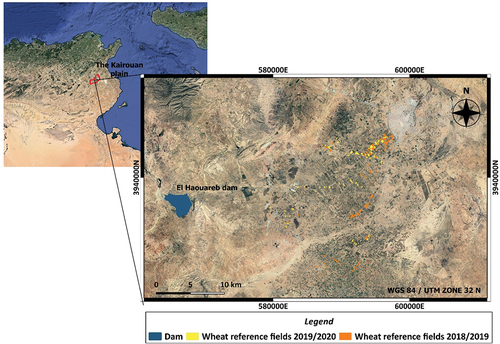
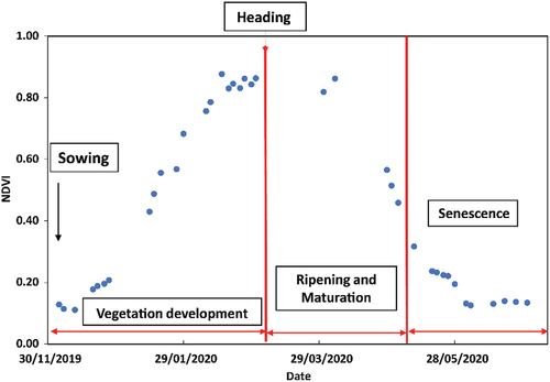
Wheat cultivation is an agricultural practice that consumes the most irrigation water due to its importance in regional and national agricultural production. Therefore, optimizing the irrigation needs of wheat depending on vegetation-growth stages is a key component of water resource management. The present study monitored the wheat cycle for two years (2018–2019 and 2019–2020), including the different phenological phases: vegetation development, heading, ripening and senescence. The cycle starts with sowing events which occur in approximately December of each year. By the end of May to June, the wheat is harvested. The observations included 64 reference fields for the first year and 66 fields in the second year. To ensure the spatial representativity of the Kairouan Plain’s agriculture scene, the area of the selected wheat fields is mostly higher than 1 hectare and can reach 13 hectares, which affords a sufficient number of pixels for calculating the average of SAR and optical data. Different surveys were held with agriculture about farming practices. The comparison between the practices revealed that each field is different in terms of wheat variety, irrigation doses and soil tillage, which decreases the interfiled spatial autocorrelation. The wheat fields are irrigated by sprinklers. Unfortunately, at the field scale, the quantification of the irrigation amount remains challenging. The study area is characterized by highly diversified small family farms that manage their practices according to their own logic (Ameur, Amichi, and Leauthaud 2020). Due to these informal arrangements, the installed irrigation systems and strategy are different from one agriculture to another which complicates quantifying the total amount of irrigation per field.

2.2. Datasets

2.2.1. Sentinel-1

To monitor and map land surfaces, the Sentinel-1 mission offers a long time series of high-spatial-resolution, SAR images operating at a center frequency of 5.405 GHz over 175 orbits. With the launch of Sentinel-1 A and B in 2014 and 2016, respectively, C-band images are available every 6 days acquired in different modes: interferometric wide-swath mode (IW), wave mode (WV), strip-map mode (SM) and extra wide-swath mode (EW). Various Sentinel-1 data products have been distributed, including raw Level-0 data, single look complex (SLC) imagery, ground range-detected (GRD) Level-1 data and Level-2 ocean (OCN) data (Torres et al. 2012).

In the present study, we used GRD and SLC Sentinel-1 images covering two wheat cycles, 2018–2019 (60 acquisitions) and 2019–2020 (56 acquisitions), over the reference fields on the Kairouan Plain, as described in Table 1. To maximize the use of the available C-band time series information as recommended by (Defourny et al. 2019), we merged the ascending and descending orbit data. In this work, the SAR data were acquired at incidence angles varying between approximately 39° and 40° for the two orbits over a flat landscape. Based on the vegetation isotropy within the wheat fields, we can assume that the difference of 1° and the limited slope variation in the study area minimize the azimuthal anisotropy for backscattering data, especially because the aforementioned problem is caused by the orientation of the topography’s slope (Schaufler et al. 2018). We used the already processed GRD images to calculate the IN, and we processed the SLC images to compute the interferometric coherence ${\rho }_{\mathit{pq}}$. All the processing steps and the calculations are detailed in the appendices.

Table 1. Characteristics of the satellite images used: optical images acquired by Sentinel-2A/B and C-band SAR images acquired by Sentinel-1A/B.

	Number of fields	Sentinel-2A/B			Sentinel-1A/B
		Number of acquisitions	Relative orbit	Revisit time	Product type	Pixel spacing Range × azimuth (m)	Number of acquisitions	Relative orbit	Revisit time
2018–2019	64	35	22 and 122	5 days	SLC GRD	2.3 × 13.9 10 × 10	60 60	88 and 95	6 days
2019–2020	66	39			SLC GRD	2.3 × 13.9 10 × 10	56 56

2.2.2. Sentinel-2

After the launch of two polar-orbiting satellites, Copernicus Sentinel-2A/B, on 23 June 2015 and 7 March 2017, respectively, high-resolution multispectral optical images with a revisit frequency of 5 days were available with a swath-width band of 290 km and spatial resolutions of 10, 20 and 60 m (Drusch et al. 2012).

Sentinel-2 bands of 10 and 20 m, depending on the spectral bands, were automatically processed by the MAJA processor of the THEIA land data center to correct the data for atmospheric effects and detect clouds (https://theia.cnes.fr/atdistrib/rocket/#/search?collection=SENTINEL2). The NDVI calculation is detailed in the supplemental section.

2.3. Methodology

As mentioned in the previous section, we attempted to investigate the moving averages coherence and IN potential to estimate the NDVI values over the wheat-growth stages. In this section, we detail the steps to predict the NDVI cycle over wheat fields using various empirical models. Thus, for each wheat field, we calculated a moving average of the extracted variables (coherence and normalized VH/VV cross-polarization ratio) with a window of 6 observations. During the remainder of the study, we used IN, ${\rho }_{\mathit{VV}}$ and ${\rho }_{\mathit{VH}}$ abbreviations to indicate the moving averages of the normalized VH/VV cross-polarization ratio, the coherence in VV and the coherence in VH, respectively. Since optical sensor acquisition is dependent on weather and is impaired especially by cloud cover, the availability of Sentinel-2 data was challenging throughout the wheat cycle and created a serious data gap in the cycle. Therefore, in the case of the absence of optical data, we calculated NDVI values using linear interpolation for each S-1 acquisition date. To minimize the irregularities of inter-fields agricultural practices and the climate conditions due to precipitation events irregularities characterizing the semiarid climate and to vary the study cases for training, we mixed data from the 2 years for NDVI estimation. The NDVI prediction strategy is based on the phenological growth stages of wheat, as we identified in appendices' section: the first period was from December to the middle of March, and the second period extended the senescence stage to June. To identify the limit between the maturation and senescence sub-periods of the second period, we used an NDVI threshold equal to ($\mathit{NDV}{I}_{\mathit{max}}-\mathit{NDV}{I}_{\mathit{min}})\ast 50\mathrm{\%}$ (Bouras et al. 2020; Chu et al. 2014). In the present case, the NDVI threshold is equal to 0.4. The second period was subdivided according to NDVI values: less than 0.4 and higher than or equal to 0.4.

To estimate the NDVI values for each period, several methods were tested utilizing curve-fitting equations and machine learning regressors, such as random forest (RF) and support vector machine (SVR). According to the literature, random forest regression (RF), support vector regression (SVR) and artificial neural networks (ANNs) are the most commonly used machine learning regression algorithms to estimate vegetation biophysical variables. When the number of samples is limited, using the ANN does not accurately estimate the objective variable. Therefore, the RF and SVR algorithms are more privileged (Balabin and Lomakina 2011; Salcedo-Sanz et al. 2020; Shataee et al. 2012). The aforementioned algorithms proved their pertinence in addressing complex relationships to estimate crop biovariables such as biomass (Mutanga, Adam, and Cho 2012; Wang et al. 2016), fractional vegetation cover (Liu et al. 2021), and leaf nitrogen content (Liang et al. 2018). In the present paper, we investigate the potential of these two algorithms to estimate the NDVI using radar data.

We randomly divided the reference field cycles and their corresponding satellite datasets into three sets: training (70% of the fields), validation (20% of the fields) and testing (10% of the fields). Each wheat cycle per set is subdivided according to the aforementioned periods (Figure A1): the first period from December to the middle of March, and the second period from the middle of March to June which is subdivided also into two sub-periods according to the NDVI threshold equal to 0.4. For each period and sub-period of the cycle, we train the model as a first step using the training data part corresponding to the same period (Figure 2). After the heading (middle of March), we noticed a saturation behavior of the selected C-band variables during the wheat maturation phase when the NDVI values are higher than 0.4. This saturation can impact the training step of the model. Therefore, only for this part of the cycle (second period and NDVI ≥ 0.4), we used the entire second period dataset, from the mid of March to the end of the cycle, to train the model and estimate the NDVI values during the wheat grain maturation and filling. For each part of the cycle, the performance of the trained models is evaluated using the corresponding part of the unseen data and not included in the training process to avoid overfitting or underfitting of the constructed models. Considering of the validation dataset in the training process can induce an untrustworthy prediction model performance and its capability to be tested on different datasets (Jabbar Rafiqul Zaman Khan and Haider 2015; Langley and Simon 1995; Li et al. 2017).

Figure 2. Flowchart of the methodology to estimate NDVI values.

2.3.1. Curve-fitting equations

To predict the NDVI during the first period, the linear relationship parameters (a and b) and the SAR parameter values were used to estimate the optical index. The constructed trained models were used to estimate the NDVI values. For the second period of the cycle describing the reproductive phase until the harvest of the wheat between the middle of March and June, we proposed two subperiods depending on the maturity phase start highlighted by the NDVI value threshold. For the second part of the cycle, the established curve-fitting equations were based on the behavior of NDVI as function of the SAR variables as illustrated in Figure 4 of the paper. Additionally, the exponential behavior was observed in the already established relationships between the Sentinel-1 variables (Interferometric coherence and cross-polarization ratio) and the NDVI values in Ouaadi et al. (2021) during the entire wheat cycle over semi-arid zone in Morocco. When the NDVI values were under 0.4, we used an exponential function for data fitting, in which we had two parameters (a and b) to calibrate and validate using the IN and the interferometric coherence separately as vegetation descriptors. For NDVI values higher than or equal to 0.4, the curve fitting equations’ approach was dependent on the type of variable, whether the VH/VV cross-polarization ratio or the coherence at the VV channel, due to the different behaviors of SAR parameters in this period. Therefore, the NDVI was retrieved using one of the following equations, where a, b, k, and k’ are parameters to calibrate and validate:

(1) $\mathrm{NDVI}=\left\{\begin{array}{c}\mathit{a}\times exp\left(\mathit{b}\times \mathit{x}\right),\mathit{NDVI}<0.4,\mathit{x}=\mathit{IN}\mathit{or}{\rho }_{\mathit{VV}}\\ \mathit{k}\times (\frac{1}{log\left(\mathrm{x}\right)})+0.15,\mathit{NDVI}\ge 0.4,\mathit{x}=\mathit{IN}\\ k^{\prime }\times (-log(\mathrm{x}))-0.15,\mathit{NDVI}\ge 0.4,\mathit{x}={\rho }_{\mathit{VV}}\end{array}\right.$(1)

2.3.2. Random forest regressor

The random forest algorithm is known as an efficient method for building nonlinear regression models. It is based on a random selection of trees thanks to the bootstrap aggregating method. At each tree node, the data are split as a function of the used feature values. To find the cutoff point and the best splitting point, a split criterion is measured by the residual sum squared (Breiman 2001). When the sample values are higher than the cutoff point, they are directed to the right or left node. This process is carried out until the sample moves from the root node to the terminal leaves of the selected tree, where we obtain the predicted value of the samples (Izquierdo-Verdiguier and Zurita-Milla 2020). The overall prediction is the average of the terminal leaf predictions of each tree in the forest.

In the present study, the moving averages of the coherence and cross-polarization IN were the aforementioned candidates. Therefore, we attempted to examine the contribution of each feature in the regression model. While the machine algorithm builds the model, various parameters control the structure of individual trees in the forest to retrieve the NDVI values with high prediction performance. To find the optimal hyperparameters, the RF algorithm needs to be tuned. We attempted to optimize the RF hyperparameters, such as the number of generated decision trees (10,50,100,200,300,400,500,1000) and the maximum depth of the trees (1,2,5,10,20,30,40,50,100) (Aniruddha, Fabian Ewald Fassnacht, and Kochb 2014; Izquierdo-Verdiguier and Zurita-Milla 2020) and the maximum number of features for each node of the tree. Hence, we used a grid search strategy for hyperparameters tuning step, in which we evaluated the performance of each combination of maximum depth, and the number of trees in the present case using a 3-fold cross-validation method (Gleason and Im 2012; Pelletier et al. 2016).

2.3.3. Support vector regressor

As noted in previous studies, the SVM algorithm can be used for regression analyses as a supervised-learning approach. SVM builds a model function by drawing a hyperplane that separates the observations into partitions situated at equal and maximum distances from them due to its abilities to analyze data and recognize patterns (Mountrakis, Im, and Ogole 2011; Smola and Scholkopf 2004; Zhang and Zhang 2002). The nearest points to the aforementioned plane constitute the support vectors separated by the maximum margin.

The predicted NDVI values are calculated based on the hyperplane side where the new observations are classified. The model bases its training on a loss function that equally penalizes high and low mis-retrieve values. To find the best model function, especially in nonlinear cases, kernels are used to transform the data to a higher-dimensional space to be linear and facilitate the separation between them. In this study, we involved three kernel functions: linear kernel, polynomial function, and Gaussian radial basis function (RBF), which depend on the data specifications used with the lowest regression error (Pasolli, Notarnicola, and Bruzzone 2011; Rains et al. 2022). Using the grid search strategy, we attempted to optimize the algorithm by varying the kernels (RBF, polynomial or linear functions), the kernel coefficients (gamma = 1, 0.1, 0.01, 0.001, 0.0001) and the regularization parameters (C = 1e0, 1e1, 1e2, 1e3). The same hyperparameter tuning strategy was applied for SVR using the 3-fold cross-validation method to identify the best parameters.

2.3.4. Statistical metrics

To assess the performance of the used models to estimate NDVI, we used three statistical metrics determination coefficient R², $\mathit{Bias}$, root mean square of error $\mathit{RMSE}$ and the relative RMSE (RMSEr) calculated using Equations (2)(2) $R^2=1-\frac{\sum _{\mathit{i}=1}^N{\left(x_i-x_{\mathit{predicted},\mathit{i}}\right)}^2}{{\sum }_{i=1}^N{\left(x_i-\bar{x}\right)}^2}$(2) –(5(5) $\mathrm{RMSEr}=\mathit{\hspace{0.17em}}\left(\frac{\mathrm{RMSE}}{{\mathit{x}}_{\mathit{max}}-x_{\mathit{min}}}\right)\mathit{\hspace{0.17em}}\times \mathit{\hspace{0.17em}}100$(5) ):

(2) $R^2=1-\frac{\sum _{\mathit{i}=1}^N{\left(x_i-x_{\mathit{predicted},\mathit{i}}\right)}^2}{{\sum }_{i=1}^N{\left(x_i-\bar{x}\right)}^2}$(2)

(3) $\mathrm{Bias}=\mathit{\hspace{0.17em}}\frac{1}{\mathit{N}\mathit{\hspace{0.17em}}}\mathit{\hspace{0.17em}}\sum _{\mathit{i}=1}^N\left(x_{\mathit{predicted},\mathit{i}}-\mathit{\hspace{0.17em}}{x}_{\mathit{observed},\mathit{i}}\right)$(3)

(4) $\mathit{RMSE}=\sqrt{\frac{1}{N}\mathit{\hspace{0.17em}}\sum _{\mathit{i}=1}^N{\left({\mathit{x}}_{\mathit{predicted},\mathit{i}}-\mathit{\hspace{0.17em}}{x}_{\mathit{observed},\mathit{i}}\right)}^2}$(4)

(5) $\mathrm{RMSEr}=\mathit{\hspace{0.17em}}\left(\frac{\mathrm{RMSE}}{{\mathit{x}}_{\mathit{max}}-x_{\mathit{min}}}\right)\mathit{\hspace{0.17em}}\times \mathit{\hspace{0.17em}}100$(5)

where $x_{\mathit{predicted},\mathit{i}}$ and $x_{\mathit{observed},\mathit{i}}$ are the predicted and observed values of NDVI, respectively, of sample i of the total samples N, $\bar{x}=\frac{1}{N}{\sum }_{i=1}^N{x}_i$ and $x_{\mathit{max}}$ and $x_{\mathit{min}}$ are, respectively, the maximum and the minimum of the observed NDVI values.

3. Results

3.1. NDVI and radar variable dynamics during the wheat cycle

Figure 3a,b display the boxplots of the moving averages of the interferometric coherence in VV and VH polarizations and the VH/VV cross-polarization ratio and the interpolated NDVI dynamics during the wheat-growth cycle. Throughout the 2 years, the NDVI values increased continuously until a saturation phase, which was characterized by small value fluctuations. The plateau was reached, recording the highest NDVI values, which characterize the combined effect of the maximum chlorophyll content consequently highly photosynthetic vegetation and vegetation density. The boxplots show high variation in the NDVI values at the start of the cycle, and these differences may have been induced by the different agricultural practices in the study zone, especially the sowing dates, which vary between November and January. After the saturation phase, the NDVI values decreased with wheat maturation, describing the chromatic changes until the harvest event at the end of the cycle, in which the NDVI values were stable at approximately 0.2, indicating the absence of vegetation.

Figure 3. Boxplots of the moving average of IN, ${\rho }_{\mathit{VV}}$, ${\rho }_{\mathit{VH}}$ and the interpolated NDVI during the wheat-growth cycles: (a) 2018/2019 and (b) 2019/2020 marked by the growth stages: heading (blue dashed line) and senescence start (orange dashed line).

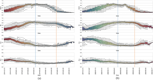
Regarding the VH/VV cross-polarization ratio index, its curve has the same trends as the NDVI curve, especially from the start of the NDVI cycle until saturation. Despite the decrease in NDVI values, the IN values remained high due to the volume-scattering effect and the water content of vegetation during the wheat maturation phases. The interferometric coherence values varied between 0.15 and 0.77 for copolarization and between 0.15 and 0.52 for VH polarization and inversely affected the NDVI evolutionary curve. The coherence trends were marked by the relative discrepancies marking the start of the vegetation cycle and the harvesting event at the end of the cycle. This behavior may be due to the differences between sowing and harvest timing between the fields. The lowest values of approximately 0.15 marked vegetation peak. With a dynamic range of 0.62, the coherence in VV polarization had a larger variation than the cross-polarized coherence, which varied over a dynamic range of 0.4.

3.2. NDVI and radar variable dynamics according to SAR acquisition dates

To exanimate the variation in the proposed SAR variables as an NDVI function, we made a scatterplot of the relationships between the moving averages of the coherence in VV (${\rho }_{\mathit{VV}})$ and VH $\left({\rho }_{\mathit{VH}}\right)$ polarizations, the IN and the NDVI values colored by the SAR data acquisitions during two wheat cycles (2018/2019 and 2019/2020) on the Kairouan Plain. According to Figure 4, the NDVI values vary between 0.2 and 1, in which a high density of values is recorded for the 0.8 and 0.9 intervals. The IN values range between 0.1 and 0.9 in Figures 4a,b. The coherence values fluctuate between 0.15 and 0.8 and between 0.15 and 0.5 in VV and VH polarizations, respectively. We distinguish a relative noise related using the coherence in the cross-polarization $\left({\rho }_{\mathit{VH}}\right)$. The normalized ratio values increase linearly with the increase in the NDVI in a linear way. After reaching the maximum NDVI values, the normalized ratio decreases with a hysteresis curve (Figure 4).

Figure 4. Scatterplots of the interpolated NDVI values during each S-1 acquisition as a function of the moving average of in and the coherence in VV (${\rho }_{\mathit{VV}})$ and VH polarization $\left({\rho }_{\mathit{VH}}\right)$ during the wheat-growth cycles for all the reference fields (each point is a moving average variable colored by S-1 acquisition date): (a) 2018/2019 and (b) 2019/2020.

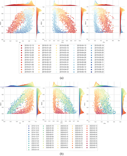
The relationships between the NDVI and the coherence are characterized by a linear part and a saturated part in which the coherence values are low, similar to the hysteresis curve. According to the kernel density estimation plot of the copolarized coherence, the saturation phase is highlighted for values between 0.2 and 0.3. By comparing the two coherence scatterplots as an NDVI function, the differentiation between the two parts of the composite curve using the coherence in VV polarization is more obvious than in the VH polarization. Therefore, in later analysis, we kept only the copolarized coherence and the IN to emphasize the relationships between the NDVI and the parameters with the minimum noise. According to the scatterplots, we observed a linear relationship characterizing the first period of the cycles starting from December until the middle of March of each cycle, in which the NDVI values increased from 0.2 to 1, indicating an increase in the chlorophyll content in vegetation and the wheat heading phase. During this period, the coherence values fluctuated between 0.2 and 0.7 and between 0.2 and 0.8 for 2018/2019 and 2019/2020, respectively. The normalized ratio index values varied between 0.1 and 0.9 during the two cycles. For the maximum NDVI values, a high density of coherence low values and IN high values characterized the scatters during March, which may indicate a saturation phase at the end of the first period. Starting from the heading event, which overlaps the middle of March, the NDVI values decreased, facing erratic variations in coherence and IN values.

The dynamics of SAR variables restarted when the vegetation organs (kernels, head and stems) turned yellow and dough. At this stage, the NDVI values were approximately less than 0.4. Therefore, we could divide the second period between mid-March and June into two subperiods depending on the start of physiological maturity; otherwise, the NDVI threshold was equal to 0.4.

3.3. NDVI estimation during the wheat cycle

In this section, we estimate the NDVI values using the aforementioned variables per period and subperiod using curve-fitting equations using either IN or the coherence and tuned machine learning algorithms such as RF and SVR using both the IN and VV coherence as features.

3.3.1. First period of the wheat cycle

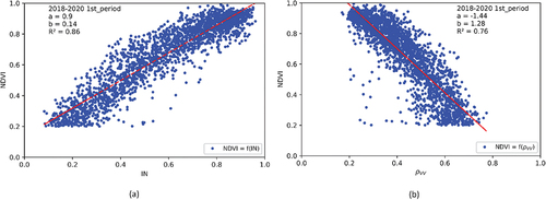
To estimate the NDVI values during the first period corresponding to vegetation growth (between sowing and the heading event), an empirical linear regression was used as a function of the VH/VV cross-polarization ratio index and the copolarized coherence with determination coefficients of 0.86 and 0.76, respectively, as displayed in Figure 5. The slope values vary between 0.9 and −1.44 for IN and ${\rho }_{\mathit{VV}}$, respectively. The order of origin values is equal to 0.14 and 1.28 for the aforementioned variables. These coefficients were used to estimate the NDVI values using the validation dataset during the first period.

Figure 5. Scatterplots of established linear relationships during the first period between the interpolated NDVI values during each S-1 acquisition and (a) in and (b) ${\rho }_{\mathit{VV}}$.

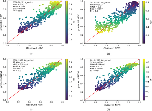
According to Figure 6a,b, high determination coefficients (R²) varying between 0.8 and 0.88 characterize the link between the estimated and observed NDVI values using the coherence and IN (as shown in Figure 5), respectively, with a maximum RMSE (RMSEr) value of 0.1(12.5%). To improve the NDVI prediction accuracy, we performed the model training of the first period using machine learning algorithms (SVR and RF), in which the coherence and VH/VV cross-polarization ratio index were the model features. Figures 6c,d display the validation of the RF with a maximum depth and number of estimators equal to 5 and 100, respectively, and the SVR with an RBF kernel. The RMSE (RMSEr) values are approximately 0.07 (8.75%), and the R² values reach a maximum of 0.9. Before reaching the maximum wheat growth, the NDVI estimation during the first period was characterized by high accuracy using the linear empirical approach as a function of the normalized index or the coherence or the machine learning regressors using both SAR variables as features. The machine learning algorithms’ estimations are validated by close accuracy. This performance is due to the obvious linearity of the relation between the SAR variables and the optical index during the first vegetation development period.

Figure 6. Scatterplots of the observed NDVI (the interpolated NDVI values during each S-1 acquisition) and predicted NDVI using an empirical linear relationship between NDVI and in (a), between NDVI and ${\rho }_{\mathit{VV}}$ (b), RF regressor algorithm with in and ${\rho }_{\mathit{VV}}$ in input (c), and (d) SVR algorithm with in and ${\rho }_{\mathit{VV}}$ in input.

3.3.2. Second period of the cycle

Using interferometric information, when the NDVI is lower than 0.4, the calibrated a and b values are equal to 0.49 and −1.95, respectively. Using the VH/VV cross-polarization ratio index, the aforementioned parameters are equal to 0.15 and 0.93, respectively. For NDVI$\ge \mathit{\hspace{0.17em}}$ 0.4, the $\mathrm{k}$ and ${\mathrm{k}}^{\prime }$ values are equal to −0.08 and 0.53, respectively. For the RF and SVR algorithms, both SAR variables (IN and ${\rho }_{\mathit{VV}}$) were used to estimate the NDVI for each subperiod. When the NDVI values were under 0.4, we could retrieve the NDVI values with RMSE values varying approximately 0.04 and 0.03 using the curve-fitting equations and RF regressor, respectively, except for the SVR algorithm case in which the RMSE reached 0.06, as illustrated in Table 2. The bias values fluctuate between −0.004 and 0.03. When the NDVI values reach 0.4, the proposed approaches underestimate the NDVI values with biases varying between −0.04 and −0.13. In this case, the SVR algorithm with an RBF kernel RF regressor with a maximum depth of 5 and number estimator of 400 relatively outperforms the curve-fitting equations with an RMSE (RMSEr) value equal to 0.17 (21.25%) compared to 0.19 (23.75%) using the curve-fitting equation as a function of the coherence and 0.28 (35%) using the curve-fitting equation as a function of cross-polarization IN. The RF model in this part of the second period built the regression model using 67% of the information from the IN and 33% from the coherence variation. This complementarity was also noted when the NDVI values were under 0.4, and the importance of IN and the coherence were equal to 45% and 55%, respectively.

Table 2. Statistical metrics of validation step using the three approaches: the empirical approach as a function of moving averages of in and coherence, the RF algorithm and the SVR algorithm during the two parts of the second period of the wheat cycle (NDVI <0.4 and NDVI ≥ 0.4).

	Curve-fitting equations			RF algorithm	SVR algorithm
		IN	${\rho }_{\mathit{VV}}$
NDVI < 0.4	RMSE	0.04	0.04	0.03	0.06
	RMSEr (%)	5	5	3.75	7.5
	Bias	−0.004	0.002	0.002	0.03
NDVI ≥ 0.4	RMSE	0.28	0.19	0.17	0.17
	RMSEr (%)	35	23.75	21.25	21.25
	Bias	−0.13	−0.09	−0.06	−0.04

3.4. NDVI cycle reconstruction

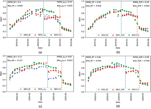
To assess the performance of the proposed approaches, we applied the approaches to estimate the NDVI and reconstruct the NDVI cycles of the 10% of fields already selected and not included in the calibration and validation steps (13 fields). Figure 7 displays the scatterplots of the observed NDVI as a function of the predicted NDVI using different approaches. The highest RMSE value is equal to 0.19 with a bias of −0.06 and the lowest R² of 0.4 characterizes the NDVI estimation using the curve-fitting equation as a function of the IN variable. The use of coherence improved the NDVI estimation with an RMSE value equal to 0.14 and R² equal to 0.67. During the wheat cycle, the machine learning algorithms relatively outperform the curve-fitting equations in which the SVR and RF show the lowest RMSE value equal to 0.12 with slight differences in the bias and the determination coefficients.

Figure 7. Scatterplots of the predicted NDVI values as a function of the observed NDVI (calculated using Sentinel-2 images) using the empirical approaches (a) NDVI=f(IN), (b) NDVI=f(${\rho }_{\mathit{VV}}$), (c) RF regressor (NDVI_RF) and (d) SVR (NDVI_SVR) using the two SAR variables (IN and ${\rho }_{\mathit{VV}})$to retrieve the NDVI wheat cycle of 13 test fields on the plain of Kairouan.

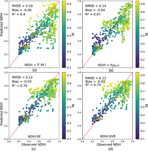
By comparing the results, we noticed that NDVI estimation using SVR is saturated, especially at the low observed NDVI values regarding high values of IN, even though the determination coefficient was equal to 0.74. This trend may be induced by the difficulty of estimating the NDVI in the second period, in which NDVI values were equal to or greater than 0.4. The difficulties of the second period are also notable in the NDVI-RF scatterplot marked by a relative noise for a range of high NDVI values. This noise is mostly pronounced with the scatterplot of the empirical approach using the cross-polarization IN with high RMSE and bias values about 0.19 and −0.06, respectively. To examine the robustness of the developed approaches, we represented the temporal NDVI dynamics of the Sentinel-2 NDVI and the estimated values. Figures 8a–d illustrate the measured NDVI cycle and the retrieved index with the different proposed methods of two of the tested fields.

Figure 8. The temporal dynamics of the observed and estimated NDVI field-average values during the wheat cycle for two selected test fields using the empirical approach (a,c) and machine learning algorithms (RF and SVR (b,d)) marked by the growth stages: heading (blue dashed line) and senescence start (orange dashed line).

According to Figure 8a, the RMSE values are equal to 0.1 and 0.13 using the curve-fitting equations as a function of IN and ${\rho }_{\mathit{VV}}$, respectively. The reconstructed NDVI cycle using calibrated equations reveals the potential of the approach to estimating the NDVI values during the first and second periods, in which the NDVI values were less than 0.4. When the NDVI values exceeded 0.4, the curve-fitting approach was unable to retrieve the same trends of the interpolated Sentinel-2 NDVI dynamics. The use of IN slightly outperformed the use of interferometric information in this case. The same difficulty was observed using the RF regressor and SVR to establish the nonlinear models in the second period and for high NDVI values. Despite the low RMSE value equal to 0.09, the saturation problem of the SVR algorithm at the end of the wheat cycle is illustrated in Figure 8b. As displayed in Figure 8c,d, the machine learning statistical metrics were better than the curve-fitting approach as a function of the IN, in which the RMSE value was approximately 0.17. Using ${\rho }_{\mathit{VV}}$, the RMSE value was equal to 0.07 with a bias value of −0.02.

4. Discussion

In the present paper, we analyzed the potential of SAR variables to reconstruct the NDVI cycle of wheat fields as a continuous crop dynamic metric independent of weather conditions. By illustrating the time series of the moving averages of the normalized polarimetric index (IN), the coherence in two channels, VV $({\rho }_{\mathit{VV}})$ and VH $\left({\rho }_{\mathit{VH}}\right)$, and the NDVI, we noticed that IN and ${\rho }_{\mathit{VV}}$ were consistent with the NDVI curve during the two wheat cycles. The IN curve, cross-polarization as already demonstrated in previous studies, was linked linearly to the NDVI for the first period of the wheat cycle until saturation when the vegetation reached its maximum green organ reflection, which overlapped with the stem elongation of wheat and the increase in the number and length of stems. In this case, as demonstrated by Veloso et al. (2017); Ouaadi et al. (2021); Palmisano et al. (2018), the backscattering coefficients in the VH channel increased with the accretion of the volume scattering. In addition, in the copolarized channel VV, the direct contribution of the bare soil and the canopy decreased due to signal attenuation with vertical structure vegetation, such as wheat, and the increase in vegetation cover fraction. As reported by Erdle et al. (2011), the NDVI values increased until the maximum wheat growth occurred in approximately the middle of March. With the start of the wheat grain filling period phase, the chromatic changes over the wheat fields anticipated the drying of the vegetation; therefore, the NDVI curve forecasted a drop before the IN curve, which remained high owing to the crop volume presence and its water content (Allies et al. 2021). The volume-scattering presence and the changes occurring in vegetation scattering were noticeable in the ${\rho }_{\mathit{VV}}$ time series more in the VH channel, which was less affected by the morphological wheat changes. The stability of the interferometric information at the start and end of the time series was interfered with by coherence loss, indicating the maximum development of the crop, which reduced the bare-soil response. The harvest event was identified by the fast increase in coherence (Alejandro et al. 2020; Arturo, Lopez-Sanchez, and Engdahl 2022). The potential of interferometric coherence in VV polarization was relevant compared to that in VH polarization in vegetation monitoring (Barbouchi et al. 2022), crop calendar identification (Arturo, Lopez-Sanchez, and Engdahl 2022), land use classification (Alejandro et al. 2020) and biophysical vegetation variable estimations, such as the case in Ouaadi et al. (2020). In the aforementioned study, the AGB of vegetation was estimated as a VV coherence function over wheat fields in semiarid areas in Morocco.

To our knowledge, the aforementioned studies examined the entire wheat cycle using the NDVI and SAR variable time series without considering the different SAR-derived variables during the phenological stages of the wheat before and after the heading and the interception of the volume-scattering and vegetation water content impact. The established empirical relations are in concordance with the already established relationships between SAR and optical data tested in semiarid regions. In the plain of Kairouan (the same study site), the relations between SAR and optical data are characterized by close accuracy and stability during different cereal growth seasons: two seasons from 2015 to 2017 in Bousbih et al. (2017) and Bousbih et al. (2018) and the 2019–2020 season in Ayari et al. (2021). In Tunisia and under the semiarid context, these relations were studied by Barbouchi et al. (2022), where the phenological stages of wheat that matched the same periods of the studied varieties with the same trends of NDVI and radar signal were identified. In another southern Mediterranean region under semiarid climate (Morocco), Ouaadi et al. (2020) and Ouaadi et al. (2021) examined these relations. By comparing the stability of NDVI and Sentinel-1 signals over wheat fields, we observed the same trends and the same period of the phenological growth stages.

The wheat cycle was divided into two parts using an empirical limit of mid-March, as detailed in the above sections. For the first period of the cycle, in which a linear relationship related the optical index to SAR parameters, RMSE values reached a maximum of 0.1, and R² values fluctuated between 0.8 and 0.9. With the increase in the vegetation cover fraction, the number of scatters increased, which impacted the link between the coherence, IN and the NDVI due to the SAR sensitivity to the fresh biomass and not just the chromatic changes. To mitigate the effect of the high density of vegetation and the complexity of the nonlinear relationships, the second period was divided according to an NDVI threshold equal to 0.4. The estimated optical index was characterized by low RMSE values of 0.06, in which the NDVI was under 0.4 during the senescence phase. If the NDVI values exceeded 0.4, the use of the IN or the coherence in the VV channel moving averages separately was limited, and the RMSE value increased beyond 0.19. The use of coherence to estimate the NDVI was more relevant than that in the IN. This may be induced due to the low sensitivity of the interferometric coherence to the soil moisture variation. According to (Ouaadi et al. 2021, 2023), during the presence of vegetation in semiarid regions, the C-band coherence is impacted by the scatter dynamics and the winds regarding a low sensitivity to precipitation and surface soil moisture. Moreover, the IN is sensitive to soil moisture and soil roughness. As discussed by Zribi et al. (2005), this aspect certainly generates noise in the signals, especially with the temporal evolution of roughness. Therefore, the use of machine learning algorithms such as RF and SVR reproduced the NDVI using the two SAR variables as complementary features. The low performance of synergy between the two SAR parameters in high vegetation density may be induced due to the saturation of the C-band signal. Using the SVR algorithm, even with low RMSE and bias values, an additional saturation problem was noticed during the senescence phase when the vegetation is dry and ready to be harvest.

The developed approach was tested on 13 wheat fields in which the entire NDVI cycle was reconstructed with an RMSE around 0.12 and an R² value approximately 0.74 using the machine learning regressors and the Sentinel-1 variables as features. Despite the potential of the RF and SVR algorithms to estimate the NDVI values, a saturation problem was highlighted in optical index time-series reconstruction using the SVR algorithm for the entire test dataset during the senescence which confirmed the aforementioned problem. Additionally, between mid-March and mid-April during the period of wheat grain filling, the NDVI estimations were saturated. This behavior confirms the complexity of optical index estimation in this period using the C-band SAR signal due to its high sensitivity to the vegetation volume and the vegetation water content. Combining Sentinel-1 descriptors, such as interferometric coherence and the normalized VH/VV cross-polarization ratio, with the reconstructed NDVI time series for wheat fields may be a solution for temperate and tropical regions suffering from a lack of optical data availability due to cloud presence and artifacts induced by sensor acquisition quality (Frantz 2019; Huang et al. 2021).

Despite the merits of the present approach, the developed empirical models require data acquisition during the entire wheat cycle. Otherwise, we need to attend to the minimum and maximum of the cross-polarization ratio to calculate the IN. Therefore, we cannot consider it a real-time application. Regarding coherence, the impact of the temporal baseline was discussed by Ouaadi et al. (2021), Arturo et al. (2022), which highlighted the importance of a short temporal baseline for coherence use. After the technical problems of Sentinel-1 B on the 23rd of December 2021, C-band images were available every 12 days. The use of 12 days leads to a less accurate temporal baseline, which escapes some structural vegetation changes. To resolve this anomaly, Sentinel-1C will be launched to replace Sentinel-1B and provide 6-day repetitiveness.

Additionally, in the present study, we considered approximate dates of sowing, harvest events and phenological stages for all the fields. According to these wheat phenophases, we divided the NDVI cycle into periods and subperiods to estimate the optical index values. This dependency on the phenological phases complicates the transferability of the methods. In fact, the proposed approach is linked to study site characteristics such as climate and farming practices. Hence, the transferability of the NDVI estimation models to another site with different climate and farming contexts requires the recalibration of the empirical models (Weiss et al. 2020; Ouaadi et al. 2023). Otherwise, we need to identify the dates of each growth stage per field. This temporal variable may be used with radar data as features to train the model using the machine learning algorithms for the entire dataset to reconstruct the NDVI cycle.

In further steps, this approach needs to be used in applications, such as vegetation biophysical variable mapping and land use classification, with high spatial and temporal resolution using the available Sentinel-1 acquisitions every 6 days. Hence, this estimated index comparable to the NDVI, may correct the vegetation volume effect in many agricultural applications, such the soil moisture estimation which is based on vegetation’s dynamic description (Ayari et al. 2021; Baghdadi et al. 2017; Bousbih et al. 2017; El Hajj et al. 2017) or FAO-56 crop coefficient monitoring (Ouaadi et al. 2023). Moreover, the optical index estimation methodology using C-band radar data may be tested on other vegetation indices (Pôças et al. 2020; Xue and Su 2017) such as the enhanced vegetation index (EVI), ratio vegetation index (RVI) and perpendicular vegetation index (PVI). Among the perspectives, the artificial neural network may be used to estimate the NDVI and minimize the bias, especially during maturation and ripening periods when the NDVI values are higher than 0.4, where the relation between the NDVI and SAR descriptors is complex. The proposed approach can be applied in a forest context based on the approved potential of C-band Sentinel-1 data to monitor vegetation phenology in a temperate mixed forest context (Frison et al. 2018).

5. Conclusions

The present study introduces an approach to reconstructing the NDVI time series over wheat fields in a semiarid area on the Kairouan Plain in the center of Tunisia. The NDVI wheat dynamics suffered gaps due to cloud presence, atmospheric disturbance and sensor capacity. By considering the independence of the SAR data from weather conditions, we tested two Sentinel-1 derived descriptors to estimate the missing NDVI values: the moving averages of the normalized VH/VV cross-polarization ratio and the coherence in VV polarization. Due to the dependency of SAR data on fresh crop biomass dynamics, NDVI estimation was performed according to the phenological stages of wheat: the first period of the vegetation development, the second period when NDVI values are higher than 0.4 and the second period with NDVI values are lower than 0.4. For each period and subperiod of the NDVI time-series, a trained model was established to estimate the NDVI values.

To retrieve the NDVI values, curve-fitting equations and RF and SVR algorithms were used. For the first growth period, using linear regression, the NDVI was estimated with RMSE values varying between 0.07 and 0.1 using the IN and coherence in VV polarization, respectively. Similar low RMSE values were observed using the regression algorithms and both SAR variables as features. For the second period, at a low level of NDVI values (NDVI <0.4), SAR variables successfully contributed to estimating the NDVI with RMSE values equal to 0.06 using SVR and 0.03 RF regressor and 0.04 using the curve-fitting equations. The use of one single SAR descriptor, IN or coherence, was insufficient to estimate the NDVI in a dense wheat context (NDVI ≥0.4), in which the RMSE (RMSEr) value varied between 0.19 (23.75%) and 0.28 (35%) with the outperformance of the coherence use. Despite the use of machine learning algorithms, the RMSE value was approximately 0.17. However, the proposed approach was applied to several test fields to estimate the NDVI values and reconstruct the optical index time series. Overall, the RMSE values varied between 0.12 and 0.19, and the determination coefficient ranged from 0.4 using the empirical model as function of IN to 0.76 using the machine learning algorithms with the IN and coherence as features.

The results confirmed the potential of Sentinel-1 derived variables to derive the NDVI values during the majority of the wheat NDVI cycle especially during vegetation development until the heading phase. During the wheat maturation and grain filling phase, low performance of the established models was observed when the vegetation volume and water content govern the radar signal scattering. The aforementioned impact on the C-band signal decreased the accuracy of the NDVI estimation especially that the optical index doesn’t consider the vegetation volume effect. This approach can be applied to other vegetation types and under different climate contexts to retrieve crop dynamics at a regional scale. In further steps, we can establish an entire mathematical approach to reconstruct the wheat NDVI cycle over a large regional spatial area where the ancillary data of phenological growth stages are available.

Highlights

• NDVI time series are reconstructed from radar polarization ratio and interferometric coherence

• NDVI values are estimated according to wheat growth stages

• Using the radar variables with the machine learning regressors improve the accuracy of NDVI estimation for testing fields by more than 36% using the curve-fitting equations as function of the polarization ratio

• For ripening and maturation period, the NDVI estimation is the most complicated.

Acknowledgment

We extend our warm thanks to the technical teams at the IRD and INAT (Institut National Agronomique de Tunisie) who participated in the ground truth measurement campaigns and data processing.

Disclosure statement

No potential conflict of interest was reported by the author(s).

Data availability statement

The data that support the findings of this study are available from the coauthor, Mehrez Zribi, upon reasonable request.

Correction Statement

This article has been republished with minor changes. These changes do not impact the academic content of the article.

Additional information

Funding

This research has been supported by the European Space Agency Climate Change Initiative for Soil Moisture (grant 4000126684/19/I-NB), the Viana (ERA-Net ARIMNet) Project, the PHC Utique IPASS Project, the Chaams (ERANET3-602 CHAAMS) Project, the Irrigation+ ((ESA n◦4000129870/20/I-NB) Project; the TAPAS TOSCA/ CNES project and H2020 ACCWA project.

Appendices

A.1. Sentinel-1

A.1.1. Single look complex Sentinel-1 data

The SLC products include complex samples preserving the amplitude and phase information in vertical – vertical (VV) and vertical – horizontal (VH) polarization channels acquired in IW mode. The C-band product contains one image per subswath with a total number of 3 subswaths. Each subswath contains various bursts in azimuth-time-order separated by black-fill demarcations. The SLC images used were downloaded from the CNES’s Sentinel Product Exploitation Platform (PEPS), which redistributes the Sentinel products generated by the European Union program for the observation and monitoring of the Earth Copernicus (https://peps.cnes.fr/rocket/#/home). The Level-1 images were processed using the SNAP Sentinel-1 toolbox to calculate the interferometric coherence following five basic steps (Ouaadi et al. 2020, 2021). After the image split and the subswath selection, the precise orbit file was applied to determine the orbit positions with an accuracy rate of less than 5 cm, at a sub-pixel level. The co-registration of two Sentinel-1 acquisitions for the same orbit (ascending or descending) is performed into a stack of master and slave images assisted by a digital elevation model SRTM DEM downloaded automatically. In the following step, the coherence ${\rho }_{\mathit{pq}}$ was computed between two consecutive acquisitions to highlight the similarities between the two image pixels using a window size of 15(Range) × 3 (azimuth) to obtain a square pixel. The coherence absolute value is computed, according to Ridha et al. (1999), as the following Equation (A1)(A1) ${\rho }_{\mathit{pq}}=\frac{\left|{\sum }_{i=1}^N{z}_{\mathit{i}}.z_i^{\prime \ast }\right|}{\sqrt{{\sum }_{i=1}^N{\left|z_i\right|}^2{\sum }_{i=1}^N{\left|z_i^{\prime }\right|}^2}}$(A1) :

(A1) ${\rho }_{\mathit{pq}}=\frac{\left|{\sum }_{i=1}^N{z}_{\mathit{i}}.z_i^{\prime \ast }\right|}{\sqrt{{\sum }_{i=1}^N{\left|z_i\right|}^2{\sum }_{i=1}^N{\left|z_i^{\prime }\right|}^2}}$(A1)

where $z_i$ and $z_i^{\prime \ast }$ are the complex number of the first SAR image and the complex conjugate number of the second SAR image, respectively, and pq is the SAR sensor polarization (VV or VH).

The ${\rho }_{\mathit{pq}}$ values vary between 0 for an incoherent pixel and 1 for perfect coherent pixels. To obtain a single image without demarcations, the TOPS deburst operator was applied followed by terrain correction to project the results in WGS 84/UTM zone 32 N based on the SRTM DEM. For each wheat field, the coherence values are averaged to obtain a mean value per field.

A.1.2. Ground Range-Detected Sentinel-1 data

GRD Sentinel-1 already processed images were downloaded from the Google Earth Engine Copernicus collection (https://developers.google.com/earth-engine/guide/sentinel1). The Earth Engine platform derived the backscattering coefficients ${\sigma }^0$per pixel in decibel (dB) in copolarization (VV) and cross-polarization (VH) after various steps of preprocessing, including orbit file application, GRD border-noise removal, thermal noise removal, radiometric calibration, and terrain correction. To avoid the disadvantages of nonadaptive or adaptive filters, we used the spatial average. Therefore, the derived ${\sigma }^0$raster was converted to a linear scale. The VH/VV cross-polarization ratio, $\frac{{\sigma }_{VH}^0}{{\sigma }_{VV}^0}$, was calculated. For each reference field, the ratio was averaged and converted to dB. As proposed by Rolle et al. (2022), the ratio values were normalized by considering the minimum and maximum ratios for each field during the wheat growth season, as detailed in Equation (A2)(A2) $\mathit{IN}=\frac{\frac{{\sigma }_{VH}^0}{{\sigma }_{VV}^0}\mathit{\hspace{0.17em}}-\mathit{\hspace{0.17em}}\frac{{\sigma }_{VH}^0}{{\sigma }_{VV}^0}{\mathit{\hspace{0.17em}}}_{\mathit{min}}}{\frac{{\sigma }_{VH}^0}{{\sigma }_{VV}^0}{\mathit{\hspace{0.17em}}}_{\mathit{max}}-\frac{{\sigma }_{VH}^0}{{\sigma }_{VV}^0}{\mathit{\hspace{0.17em}}}_{\mathit{min}}}$(A2) :

(A2) $\mathit{IN}=\frac{\frac{{\sigma }_{VH}^0}{{\sigma }_{VV}^0}\mathit{\hspace{0.17em}}-\mathit{\hspace{0.17em}}\frac{{\sigma }_{VH}^0}{{\sigma }_{VV}^0}{\mathit{\hspace{0.17em}}}_{\mathit{min}}}{\frac{{\sigma }_{VH}^0}{{\sigma }_{VV}^0}{\mathit{\hspace{0.17em}}}_{\mathit{max}}-\frac{{\sigma }_{VH}^0}{{\sigma }_{VV}^0}{\mathit{\hspace{0.17em}}}_{\mathit{min}}}$(A2)

where $\frac{{\sigma }_{VH}^0}{{\sigma }_{VV}^0}$ is the VH/VV cross-polarization ratio per field in dB and $\frac{{\sigma }_{VH}^0}{{\sigma }_{VV}^0}{\mathit{\hspace{0.17em}}}_{\mathit{max}}$ and $\frac{{\sigma }_{VH}^0}{{\sigma }_{VV}^0}{\mathit{\hspace{0.17em}}}_{\mathit{min}}$ are the maximum and minimum VH/VV cross-polarization ratio values in dB, respectively, during the wheat cycle per field in dB. The IN values range between 0 and 1, in which the VH/VV cross-polarization ratio is equal to $\frac{{\sigma }_{VH}^0}{{\sigma }_{VV}^0}{\mathit{\hspace{0.17em}}}_{\mathit{min}}$ and $\frac{{\sigma }_{VH}^0}{{\sigma }_{VV}^0}{\mathit{\hspace{0.17em}}}_{\mathit{max}}$, respectively.

A.2. Sentinel-2

To monitor the wheat dynamic changes, we calculated the mean of the NDVI per wheat field using cloud free Sentinel-2 red ($R_{\mathit{red}}$) and near-infrared ($R_{\mathit{NIR}}$) bands at central wavelengths of 665 nm and 842 nm, respectively, and 10 m spatial resolution using Equation (3)(3) $\mathrm{Bias}=\mathit{\hspace{0.17em}}\frac{1}{\mathit{N}\mathit{\hspace{0.17em}}}\mathit{\hspace{0.17em}}\sum _{\mathit{i}=1}^N\left(x_{\mathit{predicted},\mathit{i}}-\mathit{\hspace{0.17em}}{x}_{\mathit{observed},\mathit{i}}\right)$(3) established by Rouse et al. (1973):

(A3) $\mathit{NDVI}=\frac{{\mathit{R}}_{\mathit{NIR}}-R_{\mathit{red}}}{R_{\mathit{NIR}}+R_{\mathit{red}}}$(A3)

For illustration purposes, we present a scatterplot in Figure 2 of the NDVI cycle of a wheat field with the corresponding phenological stages. The wheat cycle started with a vegetative development period marked by an increase in fresh biomass. The heading event occurred in approximately mid-March according to ground truth observations and previous works in semiarid regions (Barbouchi et al. 2022; Bouras et al. 2020; Ouaadi et al. 2020). The heading phase was followed by ripening and maturation periods when the functioning of the plant was fully oriented toward filling the grains from the produced biomass. After the grain maturation, the plant is ready to be harvest by the end of May to June.

Figure A1. The NDVI profile of a selected reference wheat field in the Kairouan Plain with the corresponding phenological phases: vegetation development period, heading event, ripening and maturation period and the senescence period. The NDVI plotted data correspond to Sentinel-2 acquisition dates.

References

- Ahmad, S., A. Kalra, and H. Stephen. 2010. “Estimating Soil Moisture Using Remote Sensing Data: A Machine Learning Approach.” Advances in Water Resources 33 (1): 69–24. https://doi.org/10.1016/j.advwatres.2009.10.008.
- Alejandro, M.-Q., J. M. Lopez-Sanchez, F. Vicente-Guijalba, A. W. Jacob, and M. E. Engdahl. 2020. “Time-Series of Sentinel-1 Interferometric Coherence and Backscatter for Crop-Type Mapping.” IEEE Journal of Selected Topics in Applied Earth Observations and Remote Sensing 13:4070–4084. https://doi.org/10.1109/JSTARS.2020.3008096.
- Ali, S. A., L. Tedone, and G. De Mastro. 2015. “Optimization of the Environmental Performance of Rainfed Durum Wheat by Adjusting the Management Practices.” Journal of Cleaner Production 87 (1): 105–118. https://doi.org/10.1016/j.jclepro.2014.09.029.
- Allies, A., A. Roumiguie, J. Francois Dejoux, R. Fieuzal, A. Jacquin, A. Veloso, L. Champolivier, and F. Baup. 2021. “Evaluation of Multiorbital SAR and Multisensor Optical Data for Empirical Estimation of Rapeseed Biophysical Parameters.” IEEE Journal of Selected Topics in Applied Earth Observations and Remote Sensing 14: 7268–7283. https://doi.org/10.1109/JSTARS.2021.3095537.
- Amal, C., D. Hernández-López, R. Ballesteros, and M. A. Moreno. 2021. “Improving the Accuracy of Multiple Algorithms for Crop Classification by Integrating Sentinel-1 Observations with Sentinel-2 Data.” Remote Sensing 13 (2): 1–21. https://doi.org/10.3390/rs13020243.
- Ameur, F., H. Amichi, and C. Leauthaud. 2020. “Agroecology in North African Irrigated Plains? Mapping Promising Practices and Characterizing Farmers’ Underlying Logics.” Regional Environmental Change 20 (4). https://doi.org/10.1007/s10113-020-01719-1.
- Amri, R., M. Zribi, Z. Lili-Chabaane, B. Duchemin, C. Gruhier, and A. Chehbouni. 2011. “Analysis of Vegetation Behavior in a North African Semi-Arid Region, Using SPOT-VEGETATION NDVI Data.” Remote Sensing 3 (12): 2568–2590. https://doi.org/10.3390/rs3122568.
- Aniruddha, G., P. K. J. Fabian Ewald Fassnacht, and B. Kochb. 2014. “A Framework for Mapping Tree Species Combining Hyperspectral and LiDAR Data: Role of Selected Classifiers and Sensor Across Three Spatial Scales.” International Journal of Applied Earth Observation and Geoinformation 26 (1): 49–63. https://doi.org/10.1016/j.jag.2013.05.017.
- Arturo, V.-C., J. M. Lopez-Sanchez, and M. E. Engdahl. 2022. “Sentinel-1 Interferometric Coherence As a Vegetation Index for Agriculture.” Remote Sensing of Environment 280 (April): 113208. https://doi.org/10.1016/j.rse.2022.113208.
- Ayari, E., Z. Kassouk, Z. Lili-Chabaane, N. Baghdadi, S. Bousbih, and M. Zribi. 2021. “Cereal Crops Soil Parameters Retrieval Using L-Band ALOS-2 and C-Band Sentinel-1 Sensors.” Remote Sensing 13 (7): 1393. https://doi.org/10.3390/rs13071393.
- Baghdadi, N., M. El Hajj, M. Zribi, and S. Bousbih. 2017. “Calibration of the Water Cloud Model at C-Band for Winter Crop Fields and Grasslands.” Remote Sensing 9 (9): 1–13. https://doi.org/10.3390/rs9090969.
- Bai, Z., S. Fang, J. Gao, Y. Zhang, G. Jin, S. Wang, Y. Zhu, and J. Xu. 2020. “Could Vegetation Index Be Derive from Synthetic Aperture Radar? – the Linear Relationship Between Interferometric Coherence and NDVI.” Scientific Reports 10 (1): 1–9. https://doi.org/10.1038/s41598-020-63560-0.
- Balabin, R. M., and E. I. Lomakina. 2011. “Support Vector Machine Regression (SVR/LS-SVM) – an Alternative to Neural Networks (ANN) for Analytical Chemistry? Comparison of Nonlinear Methods on Near Infrared (NIR) Spectroscopy Data.” Analyst 136 (8): 1703–1712. https://doi.org/10.1039/c0an00387e.
- Barbouchi, M., C. Chaabani, H. Cheikh M’Hamed, R. Abdelfattah, R. Lhissou, K. Chokmani, N. Ben Aissa, M. Annabi, and H. Bahri. 2022. “Wheat Water Deficit Monitoring Using Synthetic Aperture Radar Backscattering Coefficient and Interferometric Coherence.” Agriculture 12 (7): 1032. https://doi.org/10.3390/agriculture12071032.
- Belgiu, M., and O. Csillik. 2018. “Sentinel-2 Cropland Mapping Using Pixel-Based and Object-Based Time-Weighted Dynamic Time Warping Analysis.” Remote Sensing of Environment 204 (January): 509–523. https://doi.org/10.1016/j.rse.2017.10.005.
- Belgiu, M., and L. Drăgu. 2016. “Random Forest in Remote Sensing: A Review of Applications and Future Directions.” ISPRS Journal of Photogrammetry and Remote Sensing 114:24–31. https://doi.org/10.1016/j.isprsjprs.2016.01.011.
- Bell, J. R., E. Gebremichael, A. L. Molthan, L. A. Schultz, F. J. Meyer, C. R. Hain, S. Shrestha, and K. Cole Payne. 2020. “Complementing Optical Remote Sensing with Synthetic Aperture Radar Observations of Hail Damage Swaths to Agricultural Crops in the Central United States.” Journal of Applied Meteorology and Climatology 59 (4): 665–685. https://doi.org/10.1175/JAMC-D-19-0124.1.
- Bouras, E. H., L. Jarlan, S. Er-Raki, C. Albergel, B. Richard, R. Balaghi, and S. Khabba. 2020. “Linkages Between Rainfed Cereal Production and Agricultural Drought Through Remote Sensing Indices and a Land Data Assimilation System: A Case Study in Morocco.” Remote Sensing 12 (24): 1–35. https://doi.org/10.3390/rs12244018.
- Bousbih, S., M. Zribi, M. E. Hajj, N. Baghdadi, Z. Lili-Chabaane, Q. Gao, and P. Fanise. 2018. “Soil Moisture and Irrigation Mapping in a Semi-Arid Region, Based on the Synergetic Use of Sentinel-1 and Sentinel-2 Data.” Remote Sensing 10 (12): 1953. https://doi.org/10.3390/rs10121953.
- Bousbih, S., M. Zribi, Z. Lili-Chabaane, N. Baghdadi, M. El Hajj, Q. Gao, and B. Mougenot. 2017. “Potential of Sentinel-1 Radar Data for the Assessment of Soil and Cereal Cover Parameters.” Sensors (Switzerland) 17 (11): 2617. https://doi.org/10.3390/s17112617.
- Breiman, L. 2001. “Random Forests.” Machine Learning 45. https://doi.org/10.1023/A:1010933404324.
- Chahbi, A., M. Zribi, Z. Lili-Chabaane, B. Duchemin, M. Shabou, B. Mougenot, and G. Boulet. 2014. “Estimation of the Dynamics and Yields of Cereals in a Semi-Arid Area Using Remote Sensing and the SAFY Growth Model.” International Journal of Remote Sensing 35 (3): 1004–1028. https://doi.org/10.1080/01431161.2013.875629.
- Chen, Y., R. Cao, J. Chen, L. Liu, and B. Matsushita. 2021. “A Practical Approach to Reconstruct High-Quality Landsat NDVI Time-Series Data by Gap Filling and the Savitzky–Golay Filter.” Isprs Journal of Photogrammetry & Remote Sensing 180:174–190. https://doi.org/10.1016/j.isprsjprs.2021.08.015.
- Chen, J., P. Jönsson, M. Tamura, Z. Gu, B. Matsushita, and L. Eklundh. 2004. “A Simple Method for Reconstructing a High-Quality NDVI Time-Series Data Set Based on the Savitzky-Golay Filter.” Remote Sensing of Environment 91 (3–4): 332–344. https://doi.org/10.1016/j.rse.2004.03.014.
- Chu, L., G.-H. Liu, C. Huang, and Q.-S. Liu. 2014. “Phenology Detection of Winter Wheat in the Yellow River Delta Using MODIS NDVI Time-Series Data.” https://doi.org/10.1109/Agro-Geoinformatics.2014.6910664.
- David, N., S. Giordano, and C. Mallet. 2021. “Investigating Operational Country-Level Crop Monitoring with Sentinel~1 And~2 Imagery.” Remote Sensing Letters 12 (10): 970–982. https://doi.org/10.1080/2150704X.2021.1950940.
- Defourny, P., S. Bontemps, N. Bellemans, C. Cara, G. Dedieu, E. Guzzonato, O. Hagolle, et al. 2019. “Near Real-Time Agriculture Monitoring at National Scale at Parcel Resolution: Performance Assessment of the Sen2-Agri Automated System in Various Cropping Systems Around the World.” Remote Sensing of Environment 221 (February): 551–568. https://doi.org/10.1016/j.rse.2018.11.007.
- Denize, J., L. Hubert-Moy, J. Betbeder, S. Corgne, J. Baudry, and E. Pottier. 2019. “Evaluation of Using Sentinel-1 and -2 Time-Series to Identifywinter Land Use in Agricultural Landscapes.” Remote Sensing 11 (1): 37. https://doi.org/10.3390/rs11010037.
- Dipankar, M., V. Kumar, D. Ratha, S. Dey, A. Bhattacharya, J. M. Lopez-Sanchez, H. McNairn, and Y. S. Rao. 2020. “Dual Polarimetric Radar Vegetation Index for Crop Growth Monitoring Using Sentinel-1 SAR Data.” Remote Sensing of Environment 247 (September): 111954. https://doi.org/10.1016/j.rse.2020.111954.
- Drusch, M., U. Del Bello, S. Carlier, O. Colin, V. Fernandez, F. Gascon, B. Hoersch, et al. 2012. “Sentinel-2: ESA’s Optical High-Resolution Mission for GMES Operational Services.” Remote Sensing of Environment 120 (May): 25–36. https://doi.org/10.1016/j.rse.2011.11.026.
- Duan, T., S. C. Chapman, Y. Guo, and B. Zheng. 2017. “Dynamic Monitoring of NDVI in Wheat Agronomy and Breeding Trials Using an Unmanned Aerial Vehicle.” Field Crops Research 210 (June): 71–80. https://doi.org/10.1016/j.fcr.2017.05.025.
- El Hajj, M., N. Baghdadi, M. Zribi, and H. Bazzi. 2017. “Synergic Use of Sentinel-1 and Sentinel-2 Images for Operational Soil Moisture Mapping at High Spatial Resolution Over Agricultural Areas.” Remote Sensing 9 (12): 1–28. https://doi.org/10.3390/rs9121292.
- Erdle, K., B. Mistele, and U. Schmidhalter. 2011. “Comparison of Active and Passive Spectral Sensors in Discriminating Biomass Parameters and Nitrogen Status in Wheat Cultivars.” Field Crops Research 124 (1): 74–84. https://doi.org/10.1016/j.fcr.2011.06.007.
- Ezzahar, J., N. Ouaadi, M. Zribi, J. Elfarkh, G. Aouade, S. Khabba, S. Er-Raki, A. Chehbouni, and L. Jarlan. 2020. “Evaluation of Backscattering Models and Support Vector Machine for the Retrieval of Bare Soil Moisture from Sentinel-1 Data.” Remote Sensing 12 (1): 1–20. https://doi.org/10.3390/RS12010072.
- Frantz, D. 2019. “FORCE-Landsat + Sentinel-2 analysis ready data and beyond.“ Remote Sensing 11:9. https://doi.org/10.3390/rs11091124.
- Frison, P. L., B. Fruneau, S. Kmiha, K. Soudani, E. Dufrêne, T. Le Toan, T. Koleck, L. Villard, E. Mougin, and J. P. Rudant. 2018. “Potential of Sentinel-1 Data for Monitoring Temperate Mixed Forest Phenology.” Remote Sensing 10 (12). 2049. MDPI AG. https://doi.org/10.3390/rs10122049.
- Gleason, C. J., and J. Im. 2012. “Forest Biomass Estimation from Airborne LiDAR Data Using Machine Learning Approaches.” Remote Sensing of Environment 125:80–91. https://doi.org/10.1016/j.rse.2012.07.006.
- Goodwin, A. W., L. E. Lindsey, S. K. Harrison, A. W. Goodwin, L. E. Lindsey, S. K. Harrison, and P. A. Paul. 2018. “Crop Management Estimating Wheat Yield with Normalized Difference Vegetation Index and Fractional Green Canopy Cover.” Crop, Forage & Turfgrass Management 4 (1): 1–6. https://doi.org/10.2134/cftm2018.04.0026.
- Gorrab, A., M. Ameline, C. Albergel, and F. Baup. 2021. “Use of Sentinel-1 Multi-Configuration and Multi-Temporal Series for Monitoring Parameters of Winter Wheat.” Remote Sensing 13 (4): 1–19. https://doi.org/10.3390/rs13040553.
- Haldar, D., A. Verma, S. Kumar, and P. Chauhan. 2022. “Estimation of Mustard and Wheat Phenology Using Multi-Date Shannon Entropy and Radar Vegetation Index from Polarimetric Sentinel- 1.” Geocarto International 37 (20): 5935–5962. https://doi.org/10.1080/10106049.2021.1926554.
- Homayouni, S., H. McNairn, M. Hosseini, X. Jiao, and J. Powers. 2019. “Quad and Compact Multitemporal C-Band PolSAR Observations for Crop Characterization and Monitoring.” International Journal of Applied Earth Observation and Geoinformation 74 (February): 78–87. https://doi.org/10.1016/J.JAG.2018.09.009.
- Huang, S., L. Tang, J. P. Hupy, Y. Wang, and G. Shao. 2021. “A Commentary Review on the Use of Normalized Difference Vegetation Index (NDVI) in the Era of Popular Remote Sensing.” Journal of Forest Research 32 (1): 1–6. https://doi.org/10.1007/s11676-020-01155-1.
- Huapeng, L., C. Zhang, S. Zhang, and P. M. Atkinson. 2019. “Full Year Crop Monitoring and Separability Assessment with Fully-Polarimetric L-Band UAVSAR: A Case Study in the Sacramento Valley, California.” International Journal of Applied Earth Observation and Geoinformation 74 (September 2018): 45–56. https://doi.org/10.1016/j.jag.2018.08.024.
- Izquierdo-Verdiguier, E., and R. Zurita-Milla. 2020. “An Evaluation of Guided Regularized Random Forest for Classification and Regression Tasks in Remote Sensing.” International Journal of Applied Earth Observation and Geoinformation 88 (January): 102051. https://doi.org/10.1016/j.jag.2020.102051.
- Jabbar Rafiqul Zaman Khan, K., and D. R. Haider. 2015. “Methods to Avoid Over-Fitting and Under-Fitting in Supervised Machine Learning (Comparative Study).” Computer Science, Communication and Instrumentation Devices 70 (10.3850): 978–981.
- Jacob, A. W., C. Notarnicola, G. Suresh, O. Antropov, S. Ge, J. Praks, Y. Ban, et al. 2020. “Sentinel-1 InSAR Coherence for Land Cover Mapping: A Comparison of Multiple Feature-Based Classifiers.” IEEE Journal of Selected Topics in Applied Earth Observations and Remote Sensing 13:535–552. https://doi.org/10.1109/JSTARS.2019.2958847.
- Jacquemart, M., and K. Tiampo. 2021. “Leveraging Time Series Analysis of Radar Coherence and Normalized Difference Vegetation Index Ratios to Characterize Pre-Failure Activity of the Mud Creek Landslide, California.” Natural Hazards and Earth System Sciences 21 (2): 629–642. https://doi.org/10.5194/nhess-21-629-2021.
- Jiao, X., H. McNairn, and L. Dingle Robertson. 2021. “Monitoring Crop Growth Using a Canopy Structure Dynamic Model and Time Series of Synthetic Aperture Radar (SAR) Data.” International Journal of Remote Sensing 42 (17): 6437–6464. https://doi.org/10.1080/01431161.2021.1938739.
- Jönsson, P., and L. Eklundh. 2004. “TIMESAT – A Program for Analyzing Time-Series of Satellite Sensor Data.” Computers and Geosciences 30 (8): 833–845. https://doi.org/10.1016/j.cageo.2004.05.006.
- Josef, K., O. Cartus, M. Lavalle, C. Magnard, P. Milillo, S. Oveisgharan, B. Osmanoglu, P. A. Rosen, and U. Wegmüller. 2022. “Global Seasonal Sentinel-1 Interferometric Coherence and Backscatter Data Set.” Scientific Data 9 (1): 1–16. https://doi.org/10.1038/s41597-022-01189-6.
- Kim, Y., T. Jackson, R. Bindlish, H. Lee, and S. Hong. 2013. “Monitoring Soybean Growth Using L-, C-, and X-Band Scatterometer Data.” International Journal of Remote Sensing 34 (11): 4069–4082. https://doi.org/10.1080/01431161.2013.772309.
- Koppe, W., M. L. Gnyp, C. Hütt, Y. Yao, Y. Miao, X. Chen, and G. Bareth. 2013. “Rice Monitoring with Multi-Temporal and Dual-Polarimetric Terrasar-X Data.” International Journal of Applied Earth Observation and Geoinformation 21 (1): 568–576. https://doi.org/10.1016/j.jag.2012.07.016.
- Kumar, P., R. Prasad, A. Choudhary, D. K. Gupta, V. N. Mishra, A. K. Vishwakarma, A. K. Singh, and P. K. Srivastava. 2019. “Comprehensive Evaluation of Soil Moisture Retrieval Models Under Different Crop Cover Types Using C-Band Synthetic Aperture Radar Data.” Geocarto International 34 (9): 1022–1041. https://doi.org/10.1080/10106049.2018.1464601.
- Kussul, N., M. Lavreniuk, S. Skakun, and A. Shelestov. 2017. “Deep Learning Classification of Land Cover and Crop Types Using Remote Sensing Data.” IEEE Geoscience and Remote Sensing Letters 14 (5): 778–782. https://doi.org/10.1109/LGRS.2017.2681128.
- Labus, M. P., G. A. Nielsen, R. L. Lawrence, R. Engel, and D. S. Long. 2002. “Wheat Yield Estimates Using Multi-Temporal NDVI Satellite Imagery.” International Journal of Remote Sensing 23 (20): 4169–4180. https://doi.org/10.1080/01431160110107653.
- Langley, P., and H. A. Simon. 1995. “Applications of Machine Learning and Rule Induction.” 38. http://robotics.stanford.edu/peo-.
- Leduc, C., S. B. E. N. Ammar, G. Favreau, R. Beji, and R. Virrion. 2007. “Impacts of hydrological changes in the Mediterranean zone: environmental modifications and rural development in the Merguellil catchment, central Tunisia 52 (June 2008): 1162–1178. https://doi.org/10.1623/hysj.52.6.1162.
- Liang, L., L. Di, T. Huang, J. Wang, L. Lin, L. Wang, and M. Yang. 2018. “Estimation of Leaf Nitrogen Content in Wheat Using New Hyperspectral Indices and a Random Forest Regression Algorithm.” Remote Sensing 10 (12): 1940. https://doi.org/10.3390/rs10121940.
- Liao, L., J. Song, J. Wang, Z. Xiao, and J. Wang. 2016. “Bayesian Method for Building Frequent Landsat-Like NDVI Datasets by Integrating MODIS and Landsat NDVI.” Remote Sensing 8 (6). https://doi.org/10.3390/rs8060452.
- Li, J., K. Cheng, S. Wang, F. Morstatter, R. P. Trevino, J. Tang, and H. Liu. 2017. “Feature Selection: A Data Perspective.” ACM Computing Surveys. 50 (6): 1–45. Association for Computing Machinery. https://doi.org/10.1145/3136625.
- Liu, D., K. Jia, H. Jiang, M. Xia, G. Tao, B. Wang, and Z. Chen. 2021. “Fractional Vegetation Cover Estimation Algorithm for FY-3B Reflectance Data Based on Random Forest Regression Method.” Remote Sensing 13 (11): 1–17. https://doi.org/10.3390/rs13112165.
- Liu, X., L. Ji, C. Zhang, and Y. Liu. 2022. “A Method for Reconstructing NDVI Time-Series Based on Envelope Detection and the Savitzky-Golay Filter.” International Journal of Digital Earth 15 (1): 553–584. https://doi.org/10.1080/17538947.2022.2044397.
- Li, S., L. Xu, Y. Jing, H. Yin, X. Li, and X. Guan. 2021. “High-Quality Vegetation Index Product Generation: A Review of NDVI Time Series Reconstruction Techniques.” International Journal of Applied Earth Observation and Geoinformation. 105:102640. Elsevier B.V. https://doi.org/10.1016/j.jag.2021.102640.
- Marti, J., J. Bort, G. A. Slafer, and J. L. Araus. 2007. “Can Wheat Yield Be Assessed by Early Measurements of Normalized Difference Vegetation Index?” The Annals of Applied Biology 150 (2): 253–257. https://doi.org/10.1111/j.1744-7348.2007.00126.x.
- Massuel, S., and J. Riaux. 2017. “Surexploitation de l’eau Souterraine: Pourquoi Agite-t-Onle Drapeau Rouge? Etude de Cas Dans l’aquifère de La Plaine de Kairouan (Tunsie Centrale).” Hydrogeology Journal 25 (6): 1607–1620. https://doi.org/10.1007/s10040-017-1568-2.
- Mercier, A., J. Betbeder, J. Baudry, J. Denize, V. Leroux, J.-L. Roger, F. Spicher, and L. Hubert-Moy. 2019. “Evaluation of Sentinel-1 and -2 Time Series to Derive Crop Phenology and Biomass of Wheat and Rapeseed: Northen France and Brittany Case Studies.” 1114903 (October): 2. https://doi.org/10.1117/12.2533132.
- Minallah, N., M. Tariq, N. Aziz, W. Khan, A. Ur Rehman, S. Brahim Belhaouari, and R. Damasevicius. 2020. “On the Performance of Fusion Based Planet-Scope and Sentinel-2 Data for Crop Classification Using Inception Inspired Deep Convolutional Neural Network.” Public Library of Science ONE 15 (9): e0239746. https://doi.org/10.1371/journal.pone.0239746.
- Mountrakis, G., J. Im, and C. Ogole. 2011. “Support Vector Machines in Remote Sensing: A Review.” ISPRS Journal of Photogrammetry and Remote Sensing 66 (3): 247–259. https://doi.org/10.1016/j.isprsjprs.2010.11.001.
- Mutanga, O., E. Adam, and M. A. Cho. 2012. “High Density Biomass Estimation for Wetland Vegetation Using Worldview-2 Imagery and Random Forest Regression Algorithm.” International Journal of Applied Earth Observation and Geoinformation 18 (1): 399–406. https://doi.org/10.1016/j.jag.2012.03.012.
- Narayanarao, B., S. Dey, A. Bhattacharya, D. Mandal, J. M. Lopez-Sanchez, H. McNairn, C. López-Martínez, and Y. S. Rao. 2021. “Dual-Polarimetric Descriptors from Sentinel-1 GRD SAR Data for Crop Growth Assessment.” ISPRS Journal of Photogrammetry and Remote Sensing 178 (August): 20–35. https://doi.org/10.1016/J.ISPRSJPRS.2021.05.013.
- Naser, M. A., R. Khosla, L. Longchamps, and S. Dahal. 2020. “Using NDVI to Differentiate Wheat Genotypes Productivity Under Dryland and Irrigated Conditions.” Remote Sensing 12 (5): 5. https://doi.org/10.3390/rs12050824.
- Nasirzadehdizaji, R., F. Balik Sanli, S. Abdikan, Z. Cakir, A. Sekertekin, and M. Ustuner. 2019. “Sensitivity Analysis of Multi-Temporal Sentinel-1 SAR Parameters to Crop Height and Canopy Coverage.” Applied Sciences (Switzerland) 9 (4): 655. https://doi.org/10.3390/app9040655.
- Ouaadi, N., J. Ezzahar, S. Khabba, S. Er-Raki, A. Chakir, A. Hssaine, L. D. Bouchra, et al. 2021. “C-Band Radar Data and in situ Measurements for the Monitoring of Wheat Crops in a Semi-Arid Area (Center of Morocco).” Earth System Science Data 13 (7): 3707–3731. https://doi.org/10.5194/essd-13-3707-2021.
- Ouaadi, N., L. Jarlan, J. Ezzahar, M. Zribi, S. Khabba, E. Bouras, S. Bousbih, and P.-L. Frison. 2020. “Monitoring of Wheat Crops Using the Backscattering Coefficient and the Interferometric Coherence Derived from Sentinel-1 in Semi-Arid Areas.” Remote Sensing of Environment 251 (August): 112050. https://doi.org/10.1016/j.rse.2020.112050.
- Ouaadi, N., L. Jarlan, S. Khabba, M. Le Page, A. Chakir, S. Er-Raki, and P. L. Frison. 2023. “Are the C-Band Backscattering Coefficient and Interferometric Coherence Suitable Substitutes of NDVI for the Monitoring of the FAO-56 Crop Coefficient?” Agricultural Water Management 282:108276. https://doi.org/10.1016/j.agwat.2023.108276.
- Palmisano, D., A. Balenzano, G. Satalino, F. Mattia, N. Pierdicca, and A. Monti-Guarnieri. 2018. “Sentinel-1 Sensitivity to Soil Moisture at High Incidence Angle and Its Impact on Retrieval.” International Geoscience and Remote Sensing Symposium (IGARSS) July, 59 (9): 1430–1433. https://doi.org/10.1109/IGARSS.2018.8518613.
- Pasolli, L., C. Notarnicola, and L. Bruzzone. 2011. “Estimating Soil Moisture with the Support Vector Regression Technique.” IEEE Geoscience and Remote Sensing Letters 8 (6): 1080–1084. https://doi.org/10.1109/LGRS.2011.2156759.
- Pelletier, C., S. Valero, J. Inglada, N. Champion, and G. Dedieu. 2016. “Assessing the Robustness of Random Forests to Map Land Cover with High Resolution Satellite Image Time Series Over Large Areas.” Remote Sensing of Environment 187:156–168. https://doi.org/10.1016/j.rse.2016.10.010.
- Phan, H., T. Le Toan, A. Bouvet, L. Dao Nguyen, T. Pham Duy, and M. Zribi. 2018. “Mapping of Rice Varieties and Sowing Date Using X-Band SAR Data.” Sensors (Switzerland) 18 (2): 1. https://doi.org/10.3390/s18010316.
- Pinto, R. S., M. S. Lopes, N. C. Collins, and M. P. Reynolds. 2016. “Modelling and Genetic Dissection of Staygreen Under Heat Stress.” Theoretical and Applied Genetics 129 (11): 2055–2074. https://doi.org/10.1007/s00122-016-2757-4.
- Planque, C., R. Lucas, S. Punalekar, S. Chognard, C. Hurford, C. Owers, C. Horton, et al. 2021. “National Crop Mapping Using Sentinel-1 Time Series: A Knowledge-Based Descriptive Algorithm.” Remote Sensing 13 (5): 1–30. https://doi.org/10.3390/rs13050846.
- PôçAs, I., A. Calera, I. Campos, and M. Cunha. 2020. “Remote Sensing for Estimating and Mapping Single and Basal Crop Coefficientes: A Review on Spectral Vegetation Indices Approaches.” Agricultural Water Management 233). 106081. Elsevier B.V. https://doi.org/10.1016/j.agwat.2020.106081.
- IPCC. 2022. Climate Change 2022: Impacts, Adaptation, and Vulnerability. Contribution of Working Group II to the Sixth Assessment Report of the Intergovernmental Panel on Climate Change. Edited by Pörtner, H.-O., D. C. Roberts, M. Tignor, E. S. Poloczanska, K. Mintenbeck, A. Alegría, M. Craig, S. Langsdorf, S. Löschke, V. Möller, A. Okem, B. Rama. Cambridge University Press. Cambridge University Press. https://doi.org/10.5281/zenodo.4768833.
- Rains, D., H. Lievens, G. J. M. De Lannoy, M. F. McCabe, R. A. M. De Jeu, and D. G. Miralles. 2022. “Sentinel-1 Backscatter Assimilation Using Support Vector Regression or the Water Cloud Model at European Soil Moisture Sites.” IEEE Geoscience & Remote Sensing Letters 19:0–4. https://doi.org/10.1109/LGRS.2021.3073484.
- Rembold, F., M. Meroni, F. Urbano, A. Royer, C. Atzberger, G. Lemoine, H. Eerens, and D. Haesen. 2015. “Remote Sensing Time Series Analysis for Crop Monitoring with the SPIRITS Software: New Functionalities and Use Examples.” Frontiers in Environmental Science 3 (July): 1–11. https://doi.org/10.3389/fenvs.2015.00046.
- Ridha, T., L. Armand, J. Bruniquel, and P. W. Vachon. 1999. “Coherence Estimation for SAR Imagery.” IEEE Transactions on Geoscience and Remote Sensing: A Publication of the IEEE Geoscience and Remote Sensing Society 37 (1): 135–149. https://doi.org/10.1109/36.739146
- Rolle, M., S. Tamea, P. Claps, E. Ayari, N. Baghdadi, and M. Zribi. 2022. “Analysis of Maize Sowing Periods and Cycle Phases Using Sentinel 1&2 Data Synergy.” Remote Sensing 14 (15): 3712. https://doi.org/10.3390/rs14153712.
- Rouse, J. W., R. H. Haas, J. A. Schell, and D. W. Deering. 1973. Monitoring the Vernal Advancement and Retrogradation (Green Wave Effect) of Natural Vegetation. Progress Report RSC 1978-1, 112.
- Salcedo-Sanz, S., P. Ghamisi, M. Piles, M. Werner, L. Cuadra, A. Moreno-Martínez, E. Izquierdo-Verdiguier, J. Muñoz-Marí, A. Mosavi, and G. Camps-Valls. 2020. “Machine Learning Information Fusion in Earth Observation: A Comprehensive Review of Methods, Applications and Data Sources.” Information Fusion 63:256–272. https://doi.org/10.1016/j.inffus.2020.07.004.
- Schaufler, S., B. Bauer-Marschallinger, S. Hochstöger, and W. Wagner. 2018. “Modelling and Correcting Azimuthal Anisotropy in Sentinel-1 Backscatter Data.” Remote Sensing Letters 9 (8): 799–808. https://doi.org/10.1080/2150704X.2018.1480071.
- Schonlau, M., and R. Yuyan Zou. 2020. “The Random Forest Algorithm for Statistical Learning.” Stata Journal 20 (1): 3–29. https://doi.org/10.1177/1536867X20909688.
- Segal, M. R. 2004. “Machine Learning Benchmarks and Random Forest Regression Publication Date Machine Learning Benchmarks and Random Forest Regression.” Center for Bioinformatics and Molecular Biostatistics 15. https://escholarship.org/uc/item/35x3v9t4.
- Shataee, S., S. Kalbi, A. Fallah, and D. Pelz. 2012. “Forest Attribute Imputation Using Machine-Learning Methods and ASTER Data: Comparison of K-NN, SVR and Random Forest Regression Algorithms.” International Journal of Remote Sensing 33 (19): 6254–6280. https://doi.org/10.1080/01431161.2012.682661.
- Shi, T., and S. Horvath. 2006. “Unsupervised Learning with Random Forest Predictors.” Journal of Computational and Graphical Statistics 15 (1): 118–138. https://doi.org/10.1198/106186006X94072.
- Simon, K., N. Torbick, X. Jiao, X. Huang, L. Dingle Robertson, A. Davidson, H. McNairn, M. H. Cosh, and P. Siqueira. 2021. “Comparison Between Dense L-Band and C-Band Synthetic Aperture Radar (Sar) Time Series for Crop Area Mapping Over a Nisar Calibration-Validation Site.” Agronomy 11 (2): 273. https://doi.org/10.3390/agronomy11020273.
- Smola, A. J., and B. Schölkopf. 2004. “A Tutorial on Support Vector Regression.” Statistics and Computing 14 (3): 199–222. https://doi.org/10.1023/B:STCO.0000035301.49549.88.
- Song, X.-P., W. Huang, M. C. Hansen, and P. Potapov. 2021. “An Evaluation of Landsat, Sentinel-2, Sentinel-1 and MODIS Data for Crop Type Mapping.” Science of Remote Sensing 3:100018. https://doi.org/10.1016/j.srs.2021.100018.
- Song, Y., and J. Wang. 2019. “Mapping Winter Wheat Planting Area and Monitoring Its Phenology Using Sentinel-1 Backscatter Time Series.” Remote Sensing 11 (4): 4. https://doi.org/10.3390/rs11040449.
- Stendardi, L., S. Rune Karlsen, G. Niedrist, R. Gerdol, M. Zebisch, M. Rossi, and C. Notarnicola. 2019. “Exploiting Time Series of Sentinel-1 and Sentinel-2 Imagery to Detect Meadow Phenology in Mountain Regions.” Remote Sensing 11 (5): 1–24. https://doi.org/10.3390/rs11050542.
- Tamm, T., K. Zalite, K. Voormansik, and L. Talgre. 2016. “Relating Sentinel-1 Interferometric Coherence to Mowing Events on Grasslands.” Remote Sensing 8 (10): 1–19. https://doi.org/10.3390/rs8100802.
- Torres, R., P. Snoeij, D. Geudtner, D. Bibby, M. Davidson, E. Attema, P. Potin, et al. 2012. “GMES Sentinel-1 Mission.” Remote Sensing of Environment 120 (May): 9–24. https://doi.org/10.1016/j.rse.2011.05.028.
- Vavlas, N. C., T. W. Waine, J. Meersmans, P. J. Burgess, G. Fontanelli, and G. M. Richter. 2020. “Deriving Wheat Crop Productivity Indicators Using Sentinel-1 Time Series.” Remote Sensing 12 (15): 15. https://doi.org/10.3390/RS12152385.
- Veloso, A., S. Mermoz, A. Bouvet, T. Le Toan, M. Planells, J. François Dejoux, and E. Ceschia. 2017. “Understanding the Temporal Behavior of Crops Using Sentinel-1 and Sentinel-2-Like Data for Agricultural Applications.” Remote Sensing of Environment 199 (September): 415–426. https://doi.org/10.1016/j.rse.2017.07.015.
- Vreugdenhil, M., W. Wagner, B. Bauer-Marschallinger, I. Pfeil, I. Teubner, C. Rüdiger, and P. Strauss. 2018. “Sensitivity of Sentinel-1 Backscatter to Vegetation Dynamics: An Austrian Case Study.” Remote Sensing 10 (9): 1396. https://doi.org/10.3390/rs10091396.
- Wagenseil, H., and C. Samimi. 2006. “Assessing Spatio-Temporal Variations in Plant Phenology Using Fourier Analysis on NDVI Time Series: Results from a Dry Savannah Environment in Namibia.” International Journal of Remote Sensing 27 (16): 3455–3471. https://doi.org/10.1080/01431160600639743.
- Wang, L., X. Zhou, X. Zhu, Z. Dong, and W. Guo. 2016. “Estimation of Biomass in Wheat Using Random Forest Regression Algorithm and Remote Sensing Data.” The Crop Journal 4 (3): 212–219. https://doi.org/10.1016/j.cj.2016.01.008.
- Weiss, M., F. Jacob, and G. Duveiller. 2020. “Remote Sensing for Agricultural Applications: A Meta-Review.” Remote Sensing of Environment 236. https://doi.org/10.1016/j.rse.2019.111402.
- Xue, J., and B. Su. 2017. “Significant Remote Sensing Vegetation Indices: A Review of Developments and Applications.” Journal of Sensors 2017). 1–17. Hindawi Limited. https://doi.org/10.1155/2017/1353691.
- You, X., J. Meng, M. Zhang, and T. Dong. 2013. “Remote Sensing Based Detection of Crop Phenology for Agricultural Zones in China Using a New Threshold Method.” Remote Sensing 5 (7): 3190–3211. https://doi.org/10.3390/rs5073190.
- Yunjin, K., and J. J. Van Zyl. 2009. “A Time-Series Approach to Estimate Soil Moisture Using Polarimetric Radar Data.” IEEE Transactions on Geoscience and Remote Sensing 47 (8): 2519–2527. https://doi.org/10.1109/TGRS.2009.2014944.
- Yuzugullu, O., S. Marelli, E. Erten, B. Sudret, and I. Hajnsek. 2017. “Determining Rice Growth Stage with X-Band SAR: A Metamodel Based Inversion.” Remote Sensing 9 (5): 1–20. https://doi.org/10.3390/rs905/0460.
- Zhang, L., and B. Zhang. 2002. “Relationship Between Support Vector Set and Kernel Functions in SVM.” Journal of Computer Science and Technology 17 (5): 549–555. https://doi.org/10.1007/BF02948823.
- Zhang, B., L. Zhang, D. Xie, X. Yin, C. Liu, and G. Liu. 2016. “Application of Synthetic NDVI Time Series Blended from Landsat and MODIS Data for Grassland Biomass Estimation.” Remote Sensing 8 (1). https://doi.org/10.3390/rs8010010.
- Zhong, L., Y. Ma, M. Suhyb Salama, and Z. Su. 2010. “Assessment of Vegetation Dynamics and Their Response to Variations in Precipitation and Temperature in the Tibetan Plateau.” Climatic Change 103 (3): 519–535. https://doi.org/10.1007/s10584-009-9787-8.
- Zingale, S., P. Guarnaccia, A. Matarazzo, G. Lagioia, and C. Ingrao. 2022. “A Systematic Literature Review of Life Cycle Assessments in the Durum Wheat Sector.” Science of the Total Environment 844 (June): 157230. https://doi.org/10.1016/j.scitotenv.2022.157230.
- Zribi, M., N. Baghdadi, N. Holah, and O. Fafin. 2005. “New Methodology for Soil Surface Moisture Estimation and Its Application to ENVISAT-ASAR Multi-Incidence Data Inversion.” Remote Sensing of Environment 96 (3–4): 485–496. https://doi.org/10.1016/j.rse.2005.04.005.
- Zribi, M., A. Chahbi, M. Shabou, Z. Lili-Chabaane, B. Duchemin, N. Baghdadi, R. Amri, and A. Chehbouni. 2011. “Soil Surface Moisture Estimation over a Semi-Arid Region Using ENVISAT ASAR Radar Data for Soil Evaporation Evaluation.” Hydrology and Earth System Sciences 15 (1): 345–358. https://doi.org/10.5194/hess-15-345-2011.