Analysis of the relationship between L-band SAR backscatter and understory weed density in eucalyptus plantation forests

ABSTRACT

This study aims to reveal the relationships between understory coverage (principally, weed growth) beneath the canopies of Sumatran eucalyptus plantations and L-band backscatter data gathered by the PALSAR-2 Synthetic Aperture Radar (SAR) onboard the ALOS-2 satellite. Statistical analysis in conjunction with in situ measurements of forest structural parameters reveals that the SAR polarization ratio is significantly negatively correlated with understory coverage in forests taller than or equal to 10 m or above 2 years of age. Our field investigations confirm that a decrease in canopy coverage takes place some 2 years after transplanting, which in turn permits increased penetration (decreased attenuation) of microwave signals thereby enabling the SAR to detect changes in understory coverage. In addition, both growth and unmanaged remnants of the understory vegetation in older forests reduce evaporation from the ground, which in turn stabilizes soil-moisture levels throughout the year and allows co-polarized backscatter data (which might otherwise be dominated by soil-moisture changes) to contain significant information on the underlying vegetation. No correlation between the understory and SAR backscatter was recorded in younger forests undergoing programs of intensive weed management. This is presumably because strong canopy and trunk backscatter obscured the response from understory vegetation and because artificial changes were induced in vegetation water content as a result of the application of herbicides which in turn reduced the accuracy of some of our field measurements of understory coverage. This research nevertheless demonstrates an important potential application of active satellite microwave remote sensing. We show that satellite-based L-band SAR can be used as a tool to investigate coverage percentages of understory layers. This synoptic technique reduces the need for repeated field surveys across large areas of forest. It can enhance ecosystem assessment and improve understory coverage estimates in sparse forests and in various types of plantations.

KEYWORDS:

• ALOS-2
• PALSAR-2
• satellite microwave remote sensing
• forest structure
• understory
• forest management

1. Introduction

The total area of the earth’s surface covered by large-scale plantations has been increasing since 1990 and is projected to expand further over the next several decades to meet the needs of growing populations (Korhonen et al. 2021). Worldwide, Asia maintains the largest area of plantations (FAO 2020), with Indonesia hosting a major fraction of this coverage. However, both natural and man-made forests in Indonesia face the problem of forest fires (Tacconi, Moore, and Kaimowitz 2007), which have been increasing in both frequency and overall expanse in recent years. These destructive episodes lead to production loss and various forms of environmental damage, including soil erosion and decreased biodiversity, as well as smoke and haze pollution. The problem is particularly severe during El Niño years (Murdiyarso and Adiningsih 2006), when less than 50% of the average dry-season rainfall can be recorded (Harrison, Page, and Limin 2009).

Management of the understory layer in plantations, and specifically the control of weed growth, is important for maximizing production and preventing fires in forests (hereafter, the term “understory” is used to refer to the zone beneath the plantation forest canopy (West 2006), the vegetation of which we loosely categorize as “weeds”). It is well known that weed control following the initial planting stages provides an effective means of increasing seedling survival rate since weeds compete for sunlight, nutrients, and water (Alwi et al. 2020; George and Brennan 2002), while at the later harvest stage they encumber logging operations and lead to the more rapid spread of fire and its ensuing damage to trees (Richardson 1993). The monitoring and controlling of weed growth has therefore received considerable attention in commercial forestry (Inail et al. 2021), although to date weed density has typically been assessed by means of visual inspection by local investigators. Remote sensing has been used for some time to monitor understory vegetation because on-site surveying of large areas of forests is a time-consuming task.

Several remote sensing techniques and methods can be employed to determine the state of understory vegetation, with approaches based on Light detection and ranging (LiDAR) and synthetic aperture radar (SAR) (more specifically Tomographic SAR “TomoSAR”) showing particular promise. LiDAR, for example, has the capability to measure 3-D features on the Earth’s surface at high spatial resolution and accuracy (Goodwin, Coops, and Culvenor 2006) and so can in principle be used to quantify understory vegetation cover (L. Li et al. 2020; Melo et al. 2020; Singh, Davis, and Meentemeyer 2015; Wing et al. 2012; Xi et al. 2022). On the other hand, the operational requirements demanded by aircraft or unoccupied aerial systems (UAS) platforms (Michałowska and Rapiński 2021) mean that LiDAR generally yields only limited observational coverage and at relatively high cost, particularly when aircraft platforms are used. In addition, the shorter optical wavelengths are reflected by the canopy surface and may consequently be unable to adequately reveal the structure beneath (Mitchard et al. 2012; Stovall et al. 2021).

By contrast, it has been well established that microwave SAR operating at longer wavelengths (e.g. L-band and P-band) can penetrate forest canopies (Campbell, Wynne, and Thomas 2022) and is then strongly affected (in terms of reflection/absorption) by the underlying structures (Hajnsek and Desnos 2021): both the understory and the soil below (Henderson and Lewis 1998; Kobayashi et al. 2015, 2023; Saatchi and McDonald 1997). Moreover, SAR has the unique ability to observe the Earth’s surface under all weather conditions, which represents an important advantage in the tropics where cloud and large amounts of water vapor persist throughout the year (Flores Anderson, Herndon, and Kucera 2019). TomoSAR, which combines images in an interferometric approach, represents a recently developed radar-based method of detecting 3-D structures such as forest vertical structure (Petrou, Manakos, and Stathaki 2015). This technique, however, demands high coherency among images acquired at slightly different incidence angles, a requirement currently satisfied by single-pass airborne SAR (Shimada 2018; Tello et al. 2018), or other observational platforms in single-pass or short repeat-pass (i.e. within a few hours) mode (Pardini, Cazcarra-Bes, and Papathanassiou 2021). Space-borne SAR images acquired over intervals of several days or months are generally unsuitable for this type of forest-layer structural mapping, since they are affected by scene decorrelation due to the temporal changes that take place in the background dielectric properties. In short, LiDAR and TomoSAR are not currently optimized for the analysis of large areas of forests, due mainly to the specific requirements of their observational platforms.

On the other hand, imagery gathered by a single long-wavelength space-borne SAR can be readily used as a feasible and cost-effective means of wide-swath observation. Given that satellite radar remote sensing offers wider and consistent monitoring at spatial resolutions that are becoming finer with successive technological advancements, there arises a clear need to investigate the applicability of SAR data for understory estimation. However, specific examples of its application to the assessment of understory vegetation cover have so far been limited. This may be because various components, including ground roughness, leaves, trunks, branches, and moisture content (Henderson and Lewis 1998; Khati and Singh 2022), affect radar reflection, complicating the extraction of understory information from the backscattered signal.

The key problem is to understand single SAR backscatter behavior in terms of the composition and structure of the understory vegetation beneath the forest canopy. This represents a major challenge as the backscatter signatures from complex and irregular forests consisting of many varied scatterers are generally difficult to interpret. Thus, we have focused on SAR responses from plantation forests characterized by an uncomplicated layer structure. Our emphasis on such relatively uniform targets within highly regular plantations containing the same tree species and with even stand density means that the subsequent interpretation of the radar data is considerably simplified, as it avoids the need to consider more complicated scattering mechanisms. Accordingly, we shall discuss a potential methodology for the use of single satellite-based SAR imagery gathered over a plantation in the indirect detection and synoptic assessment of understory weed coverage.

In this study our objectives therefore focus on the use of satellite SAR data collected over a eucalyptus plantation forest in Sumatra, Indonesia in order to reveal the relationship between L-band SAR dual-pol backscatter and field-measured understory coverage. Our working hypothesis is that L-band backscatter can detect weed growth in the plantation forests under study here. We use the technique of multivariate regression to determine which forest structural attributes (canopy, trunk volume, understory) dominate the co-polarized and cross-polarized scattering. The derivation of a direct relationship between radar backscatter and understory coverage would represent a useful advance as then information of broad applicability in ecosystem monitoring and, more specifically, in the assessment of forest-floor conditions could be derived.

2. Methods

2.1. Study area

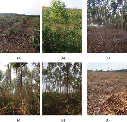
Our study focuses on plantation forests (Figure 1) in the southeast of Sumatra, Indonesia, which are managed by the forestry company “PT. Musi Hutan Persada” (PT. MHP). These holdings cover an area of 3,000 km² and are stocked with Eucalyptus pellita as a monoculture species for several years. The commercial operation of the plantation is based on ten or more sections called “Units.” Our study area is situated in Unit V, a roughly 280 km² sector extending approximately 15 km in the east-west direction and 40 km in the north-south direction. The production cycle adopted here between tree transplanting and harvesting requires four to five years (Figure 2), with most trees under 20 m in height at harvesting. The time that has elapsed since the stands were transplanted is referred to as the plantation age (hereafter referred to simply as age). Eucalyptus pellita is a fast-growing tree (Zhou et al. 2017) with an average rotation length of five to six years in the tropical regions (Nghiem 2014). Each operation of transplanting, weeding, and harvesting was performed at approximately the same time within a minimum management unit called a “forest compartment.” Overall, unit V consisted of more than 3,000 such compartments.

Figure 1. Study area in Sumatra, Indonesia shown in red rectangle. The back ground image is an SRTM30+ Global 1 km Digital Elevation Model (DEM), downloaded from the Environmental Research Division’s Data Access Program (ERDDAP). The map uses the World Geodetic system 84 (WGS 84) coordinate system.

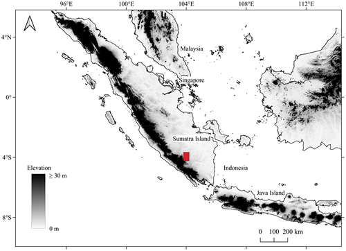
Figure 2. Plantation cycle for Eucalyptus pellita shown with plantation age (in year): (a) 0, (b) 1, (c) 2, (d) 3, (e) 4, and (f) harvested.

Grass-like weeds of Rolanda fruticose and Cyrtococcum sp. are most commonly encountered in this area (Inail et al. 2021). In addition, the wildling Acacia mangium, which was a former plantation species, can occasionally be found, although it does not thrive extensively. Weeds are managed at the ages of 3, 6, 12, 18, and 24 months for efficient timber production and fire control since, as stated above, the maintenance of relatively low surface biomass is an effective means of reducing the incidence of fire. Thereafter, weeding is not usually carried out until the harvest operation so that the understory gradually recovers. Herbicides are commonly used for weeding in younger forests, while selective tree cutting by hand is performed, if necessary, just before harvesting.

The wet season, which lasts from October to May, delivers a monthly average rainfall of 312 mm and contains two rainfall peaks in December – January and March – April. The dry season is from June to September with a monthly average rainfall of 42 mm (Inail, Hardiyanto, and Mendham 2019). The topography is hilly and lies between 60 and 200 m (Fujita, Prawiradilaga, and Yoshimura 2014) with an average elevation of approximately 80 m (Inail, Hardiyanto, and Mendham 2019).

2.2 Field observations

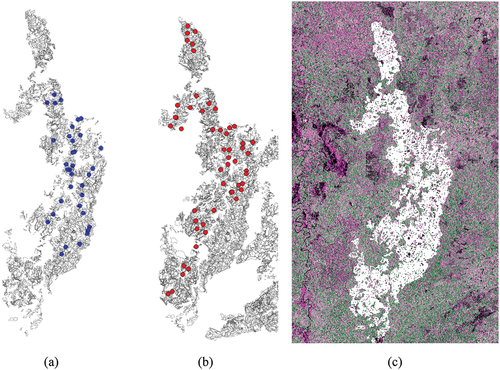
Field observations were conducted from March 1 to 4, 2019 (during the wet season) and from September 15 to 19, 2019 (dry season). Figure 3 shows the locations of the 38 and 52 sample plots used for March Figure 3(a) and September Figure 3(b), respectively. A lower sample number was obtained in this case, as the observations were difficult to conduct during the rainy season because of poor road conditions. The sample plots were distributed evenly in Unit V in spatial terms and covered all tree age groups from 0 to 5 years. However, few trees older than 5 years remained because of the harvesting strategy. Therefore, the main age group was from 0–4 years.

Figure 3. Observation sample plots (a) shown by blue circle points in March 2019 during the rainy season, and (b) shown by red circle points in September 2019 during the dry season. Background thin gray lines show forest compartment boundaries in unit V as defined by the forestry company. (c) Composite image of ALOS-2/PALSAR-2 data in March 2019 (B: HH, G: HV, R: HH/HV) with forest compartments shown by thin white lines.

In each plot, we measured three forest structural parameters: tree height (H, in m), tree diameter at breast height (DBH, in cm), and vegetation coverage (%). The observers selected 10 sample trees from which to measure the DBH and tree height with a measuring tape and clinometer, although only 5–7 trees were measured at a few sample plots (5 of 38 in March, and 2 of 52 in September) because of time constraints. The trunk volume (V, in m³) was calculated by Equation (1)(1) $\mathit{V}=\mathit{\pi }\times (\mathit{DBH}\times {10}^{-2}/2{)}^2\times \mathit{H}\times \mathit{F}$(1) :

(1) $\mathit{V}=\mathit{\pi }\times (\mathit{DBH}\times {10}^{-2}/2{)}^2\times \mathit{H}\times \mathit{F}$(1)

where F is a form factor indicative of trunk shape (set here to 0.48 (Inail, Hardiyanto, and Mendham 2019)). The tree height and trunk volume averaged for each sample plot were used in the following analyses.

Vegetation coverage (percent cover) within a circle of radius 30 m was measured by visual assessment. Several studies have used ocular inspection methods for coverage estimation in forestry (Augusto, Dupouey, and Ranger 2003; Fujita, Prawiradilaga, and Yoshimura 2014; Latifi et al. 2016; S. Li et al. 2021) as it is quicker and does not require specialized equipment, although the accuracy of these estimates depends on each observer’s experience, which can differ widely between individuals (Jennings 1999). We employed a technique based on visual estimation in order to obtain more sample data during limited field survey periods, adopting the perspective that such data can be easily comprehended by researchers in future studies. All visual assessments were conducted by a single observer (S. Kobayashi) to avoid observational bias. In addition, the Braun-Blanquet cover-abundance method was widely used during the visual assessment (Wikum and Shanholtzer 1978), in which plant communities were classified into several forest layers to assess the levels of cover abundance and sociability. This technique was applied by dividing the observed forest into four height ranges, namely: 0 − 1 m, 1 − 5 m, 5 − 10 m, and 10 − 20 m (Richards, Tansley, and Watt 1940). Tropical forests typically consist of four layers: the forest floor, the understory, the canopy, and the emergent layers (Richards, Tansley, and Watt 1940), though the latter are absent in plantation forests. The measured coverage data were then grouped and averaged as either forest canopy or understory (i.e. weed) coverages. We note that some compartments contained dead weeds as a result of herbicide application. The coverages in such instances were assumed to be 0% when appearing dry and dead, even though this vegetation remained present along the forest floor. This is because the low dielectric constant of the dried vegetation with no strong dielectric discontinuities will in turn lead to low backscatter.

The surface soil moisture content was measured with a model DM-18 digital soil moisture meter developed by Takemura Industry Co., Japan, which requires the insertion of a 2-cm long sensor into ground. The data were collected once per month between March 2019 and August 2019 from four permanent sample plots that were independent of the forest observational plots. The two younger plots of cpt 26 and cpt 27 (the abbreviation of “cpt” is used to indicate forest compartment number) contained 32 and 24 sampling points, respectively, in which data were collected three times a day at 05:30, 12:00, and 16:30 Western Indonesian Time (Waktu Indonesia Barat in Indonesian, hence WIB Time) (12:30, 19:00, and 23:30 Coordinated Universal Time: UTC). The first two of these readings (i.e. the data gathered in the morning) were then averaged for each sampling plot over the respective dates. The two older plots of cpt 15 and cpt 34 each had eight sampling points, which were measured once per day between 08:00 and 10:45 WIB (15:00 and 17:45 UTC).

Forest compartment boundaries were measured by the global positioning system (GPS) and updated constantly in accordance with the company’s daily operations. Polygon data representing the boundaries on 28 February 2019 (Figure 3(a)) and 31 August 2019 (Figure 3(b)) were used for the analyses in March and September, respectively.

2.3. Dataset and data processing

We used dual-polarization data obtained by the phased-array L-band Synthetic Aperture Radar-2 (PALSAR-2) onboard the Advanced Land Observing Satellite-2 (ALOS-2). We selected imagery acquired on the following dates and time: 10:20 WIB (17:20 UTC) on 9 March 2019 (rainy season) and 7 September 2019 (dry season) as these were closest to the dates of our field observations. Both L-band (wavelength 24.5 cm) SAR datasets were acquired during ascending orbits in fine beam dual (FBD) mode with a 34°−38° incidence angle. The dual-polarization data consist of HH and HV components, where H and V denote horizontal and vertical polarizations, respectively. Here the first character refers to the transmitted wave while the second refers to the received signal. Horizontally polarized signals are transmitted downward and subsequently return back to the sensor with zero or partial depolarization. These two components represent the co-polarized (HH) and cross-polarized (HV) returns, respectively.

These data were provided at a processing level of 1.1 by the Japan Aerospace Exploration Agency (JAXA). The original spatial resolution was about 5 m in both range and azimuth directions. In the initial stages of signal processing, radiometric calibrations (including radiometric terrain flattening) are necessary (Small 2011). Next, a boxcar speckle filter (simple moving average filter) was applied using a window size of 5 × 5 pixels equivalent to a 25 m by 25 m area. Geometric terrain correction was then carried out by resampling grids via bilinear interpolation at 5-m pixel spacing to convert the imagery into the Universal Transverse Mercator (UTM) coordinate system. The gamma naught (γ ⁰) images were finally converted into dB values, denoted as HH and HV. The HH/HV ratio, known as the cross-polarization ratio, was computed on the basis of backscattered power, rather than the logarithmically converted dB values. We used Version 8.0 of the Sentinel Application Platform (SNAP) and MATLAB 9.10 for the SAR data processing.

2.4. Statistical analysis

A statistical analysis was used to identify the forest structural attributes (canopy coverage, trunk volume, and understory coverage) that affect L-band backscatter (HH, HV, and HH/HV). This analysis was performed separately for (1) trees less than 10 m in height (referred to as younger trees) and (2) trees taller than or equal to 10 m (referred to as older trees). This division was established in the light of our preliminary research (Kobayashi and Omura 2019), which found that a change in backscatter characteristics between HH and HV components took place at approximately 10 m height. Moreover, the weeding system carried out by the company was normally adjusted after 2 years when tree heights reached ~10 m.

Firstly, the SAR parameters corresponding to the location of each field-measured forest compartment were extracted from the imagery. We excluded pixel values within 10 m of the compartmental boundary from the analysis. This edge removal procedure was adopted to minimize positional error between the satellite and the forest compartment data and to mitigate potential error due to the side-looking mode of observation of the SAR which separately images both canopy and understory of the stand. Averaged polarimetric parameters within the forest compartment’s polygon were used in the following statistical analysis. The sample size became 45 and 30 for younger and older forests, respectively after sorting the data on the basis of height, which is sufficient for unbiased multivariate regression analysis (Austin and Steyerberg 2015).

Prior to a multivariate regression analysis, the following procedures were performed. We calculated values of the logarithmically converted trunk volume with base 10 (i.e. log₁₀ Trunk volume) as a trunk parameter capable of showing linear relationships with a variety of SAR backscatters. A z-score normalization was applied to the explanatory variables, as is required for comparing the calculated slope coefficients that represent the degrees of contribution to the response variables (Roberts and Roberts 2020). Multicollinearity, which indicates high correlations among explanatory variables, was then tested by the variance inflation factor (VIF). The collinearity causes an inaccuracy in regression model development. Variables with the highest VIF value of ≥ 10 were repetitively excluded and VIF values recalculated until all variables produced VIF values < 10 (Montgomery, Peck, and Vining 2012). Following the VIF test, the forward-backward stepwise method based on the Akaike Information Criterion (AIC) approach (Kabacoff 2022) was applied to select explanatory variables that represented a best-fit model.

Lastly, the multivariate linear regression was performed with the AIC-selected variables. The results specified the slope coefficient and the p-value for selected variables, where application of hypothesis t-testing enabled us to derive the p-value under the null hypothesis that the explanatory variable had no true effect on the response variable. In addition, an adjusted R² value (Adj. R²) and a further (second) p-value were derived. The latter was obtained by F-testing under the null hypothesis that none of the explanatory variables were related to the response variables (Martin 2022). Furthermore, t-tests for association were performed on pairs of explanatory and objective variables, that were revealed to be related by the multiple regressions. We used a one-sided test by applying the correlation direction derived from estimation of the partial regression coefficients. MATLAB 9.10 and TerrSet 2020 Version 19.0.8 were employed for this aspect of the data analysis while R version 4.0.5 was used for statistical analysis.

3. Results and discussion

3.1. Field observation data in eucalyptus Plantation

In Figure 4, we present field observational data that represent averages within each survey plot. Figure 4(a) indicates a steady increase in tree height and trunk volume with plantation age. Heights reach approximately 10 m after 2 years and 20 m at around 4 years (the heights of the eucalyptus plantation trees observed within our sample plots were rarely over 20 m). Trunk volumes increase exponentially with age, with larger deviations after 2 years.

Figure 4. Field measurement data of (a) tree height (m) and trunk volume (m³), and (b) coverage (%) of forest canopy and understory with plantation age. Scatterplots show data in each forest compartment, while the line graph shows the value averaged for each age range. (c) Surface soil moisture content (%) in younger (cpt 26, 27) and older (cpt 15, 34) forest compartments are shown by the red and green lines, respectively.

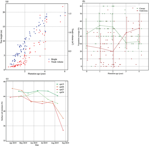
The percentage vegetation coverage in the canopy and understory with respect to age reveals varied conditions of vegetation cover among the forest compartments Figure 4(b). However, on the basis of the averaged values (lines in the graph), the canopy coverage was higher (45%–55%) and the understory coverage was lower (20%–30%) for ages below 2 years. This trend reversed after 2 years, when the canopy coverage substantially decreased to 30% while the understory coverage increased to 50%. The number of plots at age 5 years was too small to enable identification of any definite pattern. The observed understory coverage showed an opposite tendency to that in the canopy Figure 4(b), indicating that the intensive weeding over the first two years suppressed understory growth. This was followed by a cessation of weeding management and thus a subsequent recovery in the understory during the later growth period.

Visually-assessed coverages of forest canopy, in particular, have subjective tendencies compared to those of the understory because the natural variability in tree heights alters the distance between the observer and the target. The visual assessment technique, however, gave results that were consistent with those obtained by Inail, Hardiyanto, and Mendham 2019). These authors performed direct measurements on fallen eucalyptus trees in the MHP plantation which revealed that annual accumulation in leaf biomass steadily decreased after age 1 year, while the accumulation in branch biomass decreased after age 2 years (Figure 5). A direct comparison between the coverage and the biomass amounts is difficult to make; however, slower growth of canopy biomass (leaves and branches) coupled with increases in crown height likely induce a low-density canopy that would have been identified as decreased coverage in the visual observation.

Figure 5. Amount of biomass accumulation in the stand of eucalyptus pellita. modified from “growth responses of eucalyptus pellita f. muell plantations in south sumatra to macronutrient fertilisers following several rotations of acacia mangium willd.,” by M. A. Inail, Hardiyanto, and Mendham 2019, Forests, 10, 1054 (2019). Copyright (2019) by MDPI.

Figure 4(c) shows measured soil moisture content. This exhibits a similar tendency of change to that observed within the older forests (cpt 15, 34) in terms of a slight decrease during the driest season of August and September. The maximum values recorded in March (the wettest season) decline during the early dry season and fall drastically during the driest season in the younger plots (cpt 26, 27). The daily change averaged between April 2019 and September 2019 in the younger plots was 2.3% with a standard deviation of 1.2%.

The seasonal moisture change in the surface soil Figure 4(c) here was also consistent with the measured understory coverage Figure 4(b), which reflects the wetter conditions prevalent in older forests. Several hydraulic factors are influential in controlling soil moisture including rainfall and evapotranspiration, while soil properties such as runoff speed (Gonzalez et al. 2012) also play a role. However, given the distinct differences in moisture content between younger and older forests, it was concluded that evaporation rates largely determine the water content in the soil, while the wetter conditions in older forests are likely due to inhibited evaporation resulting from an increase in forest floor coverage as shown in Figure 4(b).

3.2. General scattering response of the Eucalyptus Plantation

The changes in L-band backscatter as a function of tree height are shown in Figure 6 for both rainy and dry seasons separately. The observed tendencies can be listed as follows:

Figure 6. Scatterplots between tree height (m) and L-band backscatter: (a) HH, (b) HV, and (c) HH/HV. Red and blue dots represent data for September (dry season) and March (rainy season), respectively.

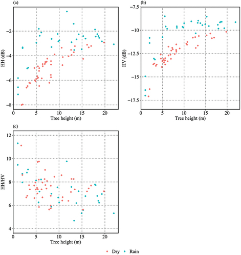
Rapid increases in HH (Figure 6(a)) and HV (Figure 6(b)) were observed up to heights of ~10 m, after which HH and HV remained relatively stable. On the other hand, HH showed greater dispersion than HV. It is well known that the primary contribution to the HH component is from double-bounce scattering generated from the trunk – ground interaction (Avtar et al. 2023; Rahman and Sumantyo 2010; Wang et al. 1995), but not from the crown – ground scattering (Figure 7) (Rahman and Sumantyo 2010). Although scattering from the trunk – ground interaction is sometimes negligible in dense forests (Kobayashi et al. 2012; Santoro et al. 2009), this is not the case in younger or sparsely covered forests as Figure 6(a) shows. The HV component is generated by multiple reflections from randomly oriented structures, such as leaves, branches, and stems (Flores Anderson, Herndon, and Kucera 2019; Sader 1987) and is thus dominated by volume scattering. In addition, (Sato et al. 2011). and Hong and Wdowinski (Hong and Wdowinski 2013) pointed out that cross-polarized backscatter consists of contributions from both double-bounce and volume scattering. Our interpretation in terms of SAR backscatter is that the HH response predominantly reflects double-bounce scattering involving the trunk and the ground, while the HV response is mainly determined by volume scattering with a partial contribution from double-bounce scattering.

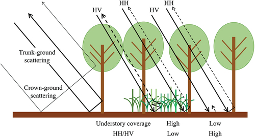
Figure 7. Schematic diagram of the double-bounce scattering which consists of trunk-ground and crown-ground scatterings. In older forests higher than 10 m, horizontally polarized waves can penetrate deeper because of the thinner forest canopy. They then generate HH returns by trunk-ground double-bounce scattering and HV returns by volume scattering. HV backscatter significantly increases with the density of understory vegetation, thereby resulting in lower HH/HV ratios.

HH Figure 6(a) and HV Figure 6(b) in the wet season were mostly higher than those in the dry season at the same tree height, as the HH/HV ratio Figure 6(c) presented a mixed distribution between dry and wet seasons and appears to be less sensitive in terms of seasonality. Thus, the effect of variability in moisture content, including soil moisture, was mitigated by using a cross ratio term (Kobayashi and Ide 2022; Veloso et al. 2017). The HH/HV ratio presents a mixed distribution pattern between the dry and rainy seasons and so offers more stable results without seasonal dependence.

3.3. Results of the statistical analysis

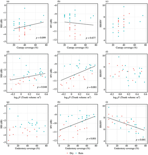
The results of multivariate regression analysis for younger (<10 m) and older forests (≥10 m) are shown in Tables 1 and 2, respectively. Scatterplots were also used to visualize the relationships between forest parameters and L-band backscatter in younger (Figure 8) and older forests (Figure 9).

Figure 8. Scatterplots between the field-measured parameters (canopy coverage, trunk volume, and understory coverage) and L-band backscatter (HH, HV, and HH/HV) for the younger forests (<10 m in tree height). The left, center, and right columns depict the explanatory variables of HH, HV, and HH/HV, respectively: (a−c) canopy coverage (%), (d−f) log₁₀ (trunk volume: m³), and (g−i) understory coverage (%). The p-values of t-tests for association are shown on the plots for pairs of variables which are selected on the basis of the multivariate regression analysis (Table 1).

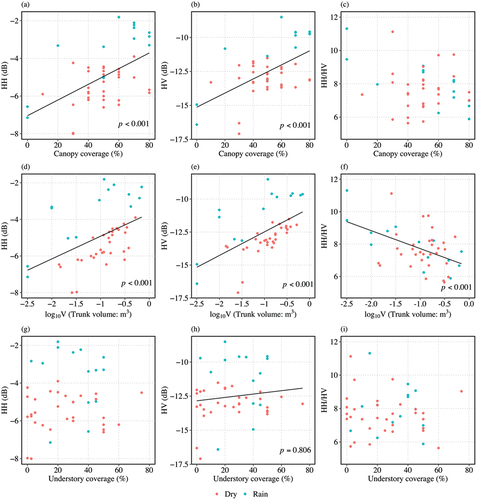
Figure 9. Scatterplots between the field-measured parameters (canopy coverage, trunk volume, and understory coverage) and L-band backscatter (HH, HV, and HH/HV) for the older forests (≥10 m in tree height). The left, center, and right columns depict the explanatory variables of HH, HV, and HH/HV, respectively: (a−c) canopy coverage (%), (d−f) log₁₀ (trunk volume: m³), and (g−i) understory coverage (%). The p-values of t-tests for association are shown on the plots for pairs of variables which are selected on the basis of the multivariate regression analysis (Table 2).

In younger forests, VIF values for the canopy coverage, trunk volume, and understory coverage were 1.24, 1.25, and 1.50, respectively and, notably, were all less than 10. AIC variable selection was then applied using all three explanatory variables. As a result of the regression analysis (Table 1), the HH signals were primarily correlated with canopy coverage (p = 0.009; Figure 8(a) and trunk volume p = 0.117; Figure 8(d) with a relatively higher Adj. R² of 0.306 (p < 0.001). In comparison, HV corresponded closely to canopy coverage (p = 0.023; Figure 8(b)), trunk volume (p = 0.007; Figure 8(e)) and understory coverage p = 0.146; Figure 8(h) with a higher Adj. R² of 0.403 (p < 0.001). Trunk volume was correlated against the HH/HV ratio p < 0.001; Figure 8(f) but gave a low Adj. R² of 0.228 (p < 0.001).

In older forests, the VIF values for canopy coverage, trunk volume, and understory coverage of 1.29, 1.15, and 1.15, respectively were again less than 10. All explanatory variables were then used in the AIC model selection. The regression analysis provided the following results (Table 2): HH showed correlation with canopy coverage p = 0.062; Figure 9(a) and trunk volume p = 0.033; Figure 9(d) with a low Adj. R² of 0.148 (p = 0.044), HV was correlated with all three parameters of canopy coverage p = 0.187; Figure 9(b), trunk volume (p = 0.013; Figure 9(e), and understory coverage (p = 0.011; Figure 9(h) and showed a higher Adj. R² of 0.371 (p = 0.002), while the HH/HV ratio corresponded solely to understory coverage (p < 0.001; Figure 9(i), producing a relatively higher Adj. R² of 0.337 (p < 0.001). Additionally, a seasonal statistical analysis was performed, and the results are shown in Appendix 12023. The understory coverage in older forests showed a stronger negative correlation with HH/HV (Adj. R² of 0.482; p = 0.001) in the rainy season (Appendix 1d). Data in the dry season (Appendix 3i) seemed to be distributed along the regression line, although the same relationship was not found in the dry season (Appendix 1c).

Table 1. Results of multivariate regression analysis for younger trees (<10 m in height). Estimates of slope coefficients and Adj. R², as well as corresponding p-values (in parentheses) are shown. Hyphens (-) indicate an explanatory variable that was not selected by the AIC metrics.

		Response variable (y)
	Parameter	HH		HV		HH/HV
Explanatory variable (x)	Canopy coverage	0.626 (0.009)**		0.605 (0.023)*		–
	Log10 trunk volume	0.366 (0.117)		0.743 (0.007)**		−0.635 (< 0.001)***
	Understory coverage	–		0.322 (0.146)		–
	Adj. R^2	0.306 (< 0.001)***		0.403 (< 0.001)***		0.228 (< 0.001)***

The p-value for each explanatory variable was calculated from t-statistics. Significance levels are denoted as follows: “*” is p < 0.050, “**” is p < 0.010, and “***” is p < 0.001.

Table 2. Results of multivariate regression analysis for older trees (≥10 m in height). Estimates of slope coefficients and Adj. R², as well as corresponding p-values (in parentheses) are shown. Hyphens (-) indicate an explanatory variable that was not selected by the AIC metrics.

		Response variable (y)
	Parameter	HH		HV		HH/HV
Explanatory variable (x)	Canopy coverage	0.307 (0.062)		0.212 (0.187)		–
	Log10 trunk volume	0.354 (0.033)*		0.398 (0.013)*		–
	Understory coverage	–		0.439 (0.011)*		−0.661 (< 0.001)***
	Adj. R^2	0.148 (0.044)*		0.371 (0.002)**		0.337 (< 0.001)***

The p-value for each explanatory variable was calculated from t-statistics. Significance levels are denoted as follows: “*” is p < 0.050, “**” is p < 0.010, and “***” is p < 0.001.

Here we aim to discuss the results of the regression analysis (Tables 1–2 and Figures 8–9) by first considering the HH and HV components in turn and by then reviewing the implications of results involving the HH/HV ratio:

(1) HH. Direct scattering from the canopy increased until age 2 years Figure 8(a). The correlation between the canopy coverage and the HH signals then became weaker in older forests Figure 9(a), as the decrease in branch density likely reduced signal response. The larger branches function as the scattering medium here, as the leaves are largely transparent to the longer-wavelength L-band signals (Rosenqvist and Killough 2018). Several studies mention that the dominant backscatter in boreal forests is direct scattering from the forest canopy (Santoro et al. 2009; Wang et al. 1993). Here, although the denseness of a typical Eucalyptus pellita canopy is relatively low, nonetheless, growing branches in the younger forests are likely responsible for the direct canopy scattering. Furthermore, the weakened correlation generally supports our visual survey of canopy coverage Figure 4(b), in revealing a decreasing branch density in older forests.

Radar penetration through the canopy increases in older forests, as branch density decreases after age 2 years. Consequently, trunk – ground double-bounce scattering increased even in older forests (Tables 1 and 2). The correlation between HH and trunk volume Figures 8(d) and 9(d) is indicative of the presence of trunk – ground double-bounce scattering. Watanabe et al. 2006) found that tree density was the main determinant of the HH backscatter. The present study did not consider tree density, as obtaining data on this parameter would have been difficult because of time and personnel constraints. Further investigation is thus required to include tree density in the program of in-situ measurements.

(2) HV. This was observed to significantly increase with canopy coverage Figure 8(b) as well as trunk volume Figure 8(e) in younger forests, as in the previous studies (Avtar et al. 2023; Kobayashi et al. 2012; Rosenqvist and Killough 2018). HV then increased with trunk Figure 9(e) and understory growth Figure 9(h) in older forests. The reduction in branch denseness, which allowed deeper signal penetration through the forest canopy, most likely increased HV backscatter from the trunk and understory. This finding is supported by Beaudoin et al. (2022). who indicated that the understory can contribute to increased volume scattering in low-volume forests.

3.4. Understory weed-density and HH/HV

Our study shows that the L-band polarimetric ratio (HH/HV) can potentially be used for understory estimation within eucalyptus plantation forests above 10 m in height. This conclusion follows from the results of the multiple regression analysis given in Table 2, in which a significant correlation was observed between the understory coverage and the HH/HV ratio. It is a reciprocal relation – larger growth in the understory implies lower HH/HV ratios (Figure 9(i)). The decreasing trend in the HH/HV ratio can likely be explained by the fact that HH levels did not change with understory growth (Figure 9(g)) whereas HV levels increased (Figure 9(h), Table 2). The increase in HV is from both trunk volume Figure 9(e) and understory Figure 9(h). However, the contribution from trunk volume is likely offset by the increase in HH with trunk volume Figure 9(d). Several studies have shown that the L-band HH component is sensitive to surface soil moisture content (El Hajj, Baghdadi, and Zribi 2019; Flores Anderson, Herndon, and Kucera 2019). Our field observations demonstrate that the soil beneath the older forest canopies maintains a relatively stable moisture content even during the dry season Figure 4(c). Accordingly, adjustments in HH backscatter presumably reflect vegetation change rather than soil moisture variations, and the HH/HV ratio consequently carries more information on vegetation. Hence, we conclude that, for taller eucalyptus forests with lower branch biomass, the HH/HV ratio contains more information on the lower levels of vegetation and so can be used to estimate the understory coverage.

Younger forests did not show any correlation with the understory coverage (Table 1, Figure 8(i)). Several possible hypotheses can be proposed to interpret these results. The lower correlation may be attributed to strong backscatter from canopies with higher branch densities and elevated trunks, which together can act to obscure the backscatter contribution from understory vegetation. Another possibility is that artificial weeding with herbicides reduced the accuracy of our coverage assessments. In the observations made here, dead weeds resulting from herbicide application were assessed as 0% coverage, even when standing vegetation remained, because the dielectric constant of dead-plant material is nearly zero. However, the weeds in such cases were often wilting but not totally withered. Therefore, the recorded understory coverages in younger forests may not reflect the actual coverage values. Enhanced canopy and trunk backscatter together with these inaccuracies in vegetation assessment could lead to decreased correlation between the understory coverage and the observed backscatter.

This study analyzed a single SAR image per season. Such minimal data coverage and analysis is insufficient to facilitate a comprehensive definition of the complex radar responses of forests. It should be also noted that the application of this research is limited to forests with thinner canopies and that the visual-inspection technique used in the assessment of vegetation cover is of limited accuracy. Nonetheless, our earlier (preliminary) study in the MHP plantation (Kobayashi and Omura 2019) supports these more recent results in demonstrating a significant correlation between understory coverage and the cross-polarization ratio. In addition, although previous studies have estimated the total above-ground biomass using satellite-based L-band SAR by making use of the capability of the radar signals to penetrate beneath forest canopies, little research has explored the independent relationship between SAR backscatter and understory conditions. This study has demonstrated a significant independent correlation between SAR response and understory coverage by focusing on a tropical plantation forest with a relatively simple layered structure.

4. Conclusions

The total area covered by plantation forests in Indonesia has been increasing. Industrial plantation companies perform rigorous weeding management to optimize production and prevent the spread of forest fires. To this end, earlier work demonstrated the potential of remote sensing techniques for determining understory (i.e. weed) conditions. The present study has explored the relationship between PALSAR-2 backscatter and field-measured forest structural parameters obtained from a eucalyptus plantation in Sumatra, Indonesia. We conducted field observations during the wet and dry seasons to measure DBH, tree height, and vegetation coverage in both the canopy and understory layers. We employed a multivariate statistical analysis to identify correlations between these forest attributes and the L-band SAR backscatter characteristics as represented by the co-polarized (HH) and cross-polarized (HV) returns and the cross-polarization ratio HH/HV.

Our results revealed that the HH/HV ratio exhibits a significant negative correlation with understory coverage in forests with trees ≥10 m in height, which results primarily from the lack of correlation of HH and the positive correlation of HV with understory coverage. The lowered branch density observed in the taller or older forests allows greater radar penetration beneath the forest canopy, facilitating stronger backscattering from surfaces nearer the ground, and thus enabling understory weed-density estimates to be made. In addition, in situ measurements show that surface soil moisture content was nearly constant within the older forests throughout the year. The recovery of the understory vegetation probably reduces evaporation from the ground and thereby stabilizes soil-moisture levels. Therefore, although the HH signal is sensitive to soil moisture variations, the HH/HV cross-polarization ratio can contain useful information on the lower levels of vegetation cover in older forests. In contrast, our results reveal the difficulty involved in understory estimation by SAR-based methods for forests <10 m in height. This was likely related to two factors: increased canopy and trunk backscatter (which reduces the understory contribution) and the use of herbicides for weeding, which artificially reduced vegetation water content, rendering the coverage assessments less accurate. Further validation with more precise in-situ observational data and a multi-year survey is clearly required. Nevertheless, this research demonstrates a potential use of satellite L-band SAR in independent understory estimation which complements its role in above-ground biomass evaluation. This new capability can provide valuable information for ecosystem assessment and should benefit forest management. Future missions employing longer-wavelength SAR (P-band) and/or fully polarimetric SAR will offer a more versatile observational approach and should lead to valuable new insights that can be used to refine the basic approach outlined in this paper.

Acknowledgments

The authors wish to thank the staff of the planning section in PT. MHP for their kind support during the field observations. We are also grateful to Mr. Koki KUBOTA (Graduate School of Agricultural and Life Sciences, the University of Tokyo) for his assistance in making the soil moisture measurements in the MHP plantation.

Disclosure statement

No potential conflict of interest was reported by the author(s).

Data availability statement

The data that support the findings of this study are available from the corresponding author upon reasonable request.

Additional information

Funding

This research was funded by JSPS KAKENHI [Grant Number 18K11626].

Appendix 1 Results of the seasonal multivariate regression analysis

(a) Younger forests (<10 m) in dry season

Table

		Response variable (y)
	Parameter	HH		HV		HH/HV
Explanatory variable (x)	Canopy coverage	0.331 (0.037)**		–	*	–
	Log10 trunk volume	1.023 (< 0.001)		1.227 (< 0.001)**		–
	Understory coverage	0.159 (0.160)		0.247 (0.089)		–
	Adj. R^2	0.593 (< 0.001)***		0.529 (< 0.001)***

(b) Younger forests (<10 m) in rainy season

Table

		Response variable (y)
	Parameter	HH		HV		HH/HV
Explanatory variable (x)	Canopy coverage	0.966 (< 0.001)**		1.376 (<0.001)*		–
	Log10 trunk volume	–		–	**	−0.810 (<0.001)***
	Understory coverage	–		–		–
	Adj. R^2	0.630 (< 0.001)***		0.670 (< 0.001)***		0.628 (< 0.001)***

(c) Older forests (≥10 m) in dry season

Table

		Response variable (y)
	Parameter	HH		HV		HH/HV
Explanatory variable (x)	Canopy coverage	0.434 (0.150)**		–		0.910 (0.049)
	Log10 trunk volume	0.403 (0.021)		0.393 (0.006)**		–
	Understory coverage	–		–		–
	Adj. R^2	0.321 (0.058)***		0.464 (0.006)***		0.244 (0.049)***

(d) Older forests (≥10 m) in rainy season

Table

		Response variable (y)
	Parameter	HH		HV		HH/HV
Explanatory variable (x)	Canopy coverage	–	**	–	*	–
	Log10 trunk volume	–		–	**	–
	Understory coverage	−0.635 (0.008)		–		−0.988 (0.001)**
	Adj. R^2	0.346 (0.008)***				0.482 (0.001)**

Appendix 2

Scatterplots between the field-measured parameters and L-band backscatter for the younger forests (<10 m in tree height). Red and blue dots represent data for September (dry season) and March (rainy season), respectively. This scatterplot is the same as the one in Figure 8, except that it is colored according to the season.

Appendix 3

Scatterplots between the field-measured parameters and L-band backscatter for the older forests (≥10 m in tree height). Red and blue dots represent data for September (dry season) and March (rainy season), respectively. This scatterplot is the same as the one in Figure 9, except that it is colored according to the season.

References

- Alwi, A., M. Lapammu, Y. Jarapudin, K. Molony, D. Boden, P. Macdonell, P. Warburton, et al. 2020. “Importance of Weed Control Prior to Planting for the Establishment of Planted Forests in Sabah.” Malaysia Journal of Tropical Forest Science 32 (4): 349–21. https://doi.org/10.26525/jtfs2020.32.4.349.
- Augusto, L., J.-L. Dupouey, and J. Ranger. 2003. “Effects of Tree Species on Understory Vegetation and Environmental Conditions in Temperate Forests.” Annals of Forest Science 60 (8): 823–831. https://doi.org/10.1051/forest:2003077.
- Austin, P. C., and E. W. Steyerberg. 2015. “The Number of Subjects per Variable Required in Linear Regression Analyses.” Journal of Clinical Epidemiology 68 (6): 627–636. https://doi.org/10.1016/j.jclinepi.2014.12.014.
- Avtar, Ram, Rashmi Malik, M. Musthafa, Virendra S. Rathore, Praveen Kumar, and Gulab Singh. 2023. “Forest Plantation Species Classification Using Full-Pol-Time-Averaged SAR Scattering Powers. Remote Sensing Applications.” Remote Sensing Applications: Society & Environment 29:100924. https://doi.org/10.1016/j.rsase.2023.100924.
- Beaudoin, A., R. J. Hall, G. Castilla, M. Filiatrault, P. Villemaire, R. Skakun, and L. Guindon. 2022. “Improved K-NN Mapping of Forest Attributes in Northern Canada Using Spaceborne L-Band SAR, Multispectral and LiDAR Data.” Remote Sensing 14 (5): 1181. https://doi.org/10.3390/rs14051181.
- Campbell, J. B., R. H. Wynne, and V. A. Thomas. 2022. Introduction to Remote Sensing, 6th ed. New York, NY: Guilford Press.
- El Hajj, M., N. Baghdadi, and M. Zribi. 2019. “Comparative Analysis of the Accuracy of Surface Soil Moisture Estimation from the C-And L-Bands.” International Journal of Applied Earth Observation and Geoinformation 82:101888. https://doi.org/10.1016/j.jag.2019.05.021.
- FAO. 2020. Global Forest Resources Assessment 2020 – Key Findings. Rome. https://doi.org/10.4060/ca8753en.
- Flores Anderson, A. I., K. E. Herndon, and L. M. Kucera. 2019. “The Synthetic Aperture Radar (SAR) Handbook: Comprehensive Methodologies for Forest Monitoring and Biomass Estimation.”
- Fujita, M. S., D. M. Prawiradilaga, and T. Yoshimura. 2014. “Roles of Fragmented and Logged Forests for Bird Communities in Industrial Acacia Mangium Plantations in Indonesia.” Ecological Research 29 (4): 741–755. https://doi.org/10.1007/s11284-014-1166-x.
- George, B., and P. Brennan. 2002. “Herbicides Are More Cost-Effective Than Alternative Weed Control Methods for Increasing Early Growth of Eucalyptus Dunnii and Eucalyptus Saligna.” New Forests 24 (2): 147–163. https://doi.org/10.1023/A:1021227913989.
- Gonzalez, R. G., A. Verhoef, P. L. Vidale, B. Main, G. Gan, and Y. Wu. 2012. “Interactions Between the Physical Soil Environment and a Horizontal Ground Coupled Heat Pump, for a Domestic Site in the UK. Renewable Energy.” Renewable Energy 44:141–153. https://doi.org/10.1016/j.renene.2012.01.080.
- Goodwin, N. R., N. C. Coops, and D. S. Culvenor. 2006. “Assessment of Forest Structure with Airborne LiDAR and the Effects of Platform Altitude.” Remote Sensing of Environment 103 (2): 140–152. https://doi.org/10.1016/j.rse.2006.03.003.
- Hajnsek, I., and Y. L. Desnos. 2021. Polarimetric Synthetic Aperture Radar: Principles and Application. Cham, Swizerland: Springer.
- Harrison, M. E., S. E. Page, and S. H. Limin. 2009. “The Global Impact of Indonesian Forest Fires.” The Biologist 56 (3): 156–163.
- Henderson, F. M., and A. J. Lewis. 1998. “Principles and Applications of Imaging Radar. Manual of Remote Sensing: Volume 2.”
- Hong, S.-H., and S. Wdowinski. 2013. “Double-Bounce Component in Cross-Polarimetric SAR from a New Scattering Target Decomposition.” IEEE Transactions on Geoscience and Remote Sensing 52 (6): 3039–3051. https://doi.org/10.1109/TGRS.2013.2268853.
- Inail, M. A., E. B. Hardiyanto, and D. S. Mendham. 2019. “Growth Responses of Eucalyptus Pellita F. Muell Plantations in South Sumatra to Macronutrient Fertilisers Following Several Rotations of Acacia Mangium Willd.” Forests 10 (12): 1054. https://doi.org/10.3390/f10121054.
- Inail, M. A., E. B. Hardiyanto, D. S. Mendham, and E. Thaher. 2021. “Growth Response to Weed Control and Fertilisation in Mid-Rotation Plantations of Eucalyptus Pellita in South Sumatra.” Indonesia Forests 12 (12): 1653. https://doi.org/10.3390/f12121653.
- Jennings, S. 1999. “Assessing Forest Canopies and Understorey Illumination: Canopy Closure, Canopy Cover and Other Measures. an International Journal of Forest Research.” Forestry 72 (1): 59–74. https://doi.org/10.1093/forestry/72.1.59.
- Kabacoff, R. I. 2022. R in Action, Third Edition: Data Analysis and Graphics with R and Tidyverse, 3rd ed. Shelter Island, New York: Manning.
- Khati, U., and G. Singh. 2022. “Combining L-Band SAR Backscatter and TanDEM-X Canopy Height for Forest Aboveground Biomass Estimation.” Frontiers in Forests and Global Change 5:156. https://doi.org/10.3389/ffgc.2022.918408.
- Kobayashi, S., M. S. Fujita, Y. Omura, D. S. Haryadi, A. Muhammad, M. Irham, and S. Shiodera. 2023. “Evaluating Threatened Bird Occurrence in the Tropics by Using L-Band SAR Remote Sensing Data.” Remote Sensing 15 (4): 947. https://doi.org/10.3390/rs15040947.
- Kobayashi, S., and H. Ide. 2022. “Rice Crop Monitoring Using Sentinel-1 SAR Data: A Case Study in Saku.” Japan Remote Sensing 14 (14): 3254. https://doi.org/10.3390/rs14143254.
- Kobayashi, S., and Y. Omura. 2019. “Evaluation of Understory Vegetation in Eucalyptus Plantation by L-Band SAR Data.” Proceedings of the 66th Conference of the Remote Sensing Society of Japan, 22–23. Saitama, Japan.
- Kobayashi, S., Y. Omura, K. Sanga-Ngoie, R. Widyorini, S. Kawai, B. Supriadi, Y. Yamaguchi, et al. 2012. “Characteristics of Decomposition Powers of L-Band Multi-Polarimetric SAR in Assessing Tree Growth of Industrial Plantation Forests in the Tropics. Remote Sensing.” Remote Sensing 4 (10): 3058–3077. https://doi.org/10.3390/rs4103058.
- Kobayashi, S., Y. Omura, K. Sanga-Ngoie, Y. Yamaguchi, R. Widyorini, M. S. Fujita, B. Supriadi, et al. 2015. “Yearly Variation of Acacia Plantation Forests Obtained by Polarimetric Analysis of ALOS PALSAR Data.” IEEE Journal of Selected Topics in Applied Earth Observations and Remote Sensing 8 (11): 5294–5304. https://doi.org/10.1109/JSTARS.2015.2487503.
- Korhonen, J., P. Nepal, J. P. Prestemon, and F. W. Cubbage. 2021. “Projecting Global and Regional Outlooks for Planted Forests Under the Shared Socio-Economic Pathways.” New Forests 52 (2): 197–216. https://doi.org/10.1007/s11056-020-09789-z.
- Latifi, H., M. Heurich, F. Hartig, J. Müller, P. Krzystek, H. Jehl, S. Dech, et al. 2016. “Estimating Over-And Understorey Canopy Density of Temperate Mixed Stands by Airborne LiDAR Data.” Forestry: An International Journal of Forest Research 89 (1): 69–81. https://doi.org/10.1093/forestry/cpv032.
- Li, L., J. Chen, X. Mu, W. Li, G. Yan, D. Xie, and W. Zhang. 2020. “Quantifying Understory and Overstory Vegetation Cover Using UAV-Based RGB Imagery in Forest Plantation.” Remote Sensing 12 (2): 298. https://doi.org/10.3390/rs12020298.
- Li, S., T. Wang, Z. Hou, Y. Gong, L. Feng, and J. Ge. 2021. “Harnessing Terrestrial Laser Scanning to Predict Understory Biomass in Temperate Mixed Forests.” Ecological Indicators 121:107011. https://doi.org/10.1016/j.ecolind.2020.107011.
- Martin, P. 2022. Linear Regression: An Introduction to Statistical Models. Thousand Oaks, California: SAGE Publications.
- Melo, A. M., C. R. Reis, B. F. Martins, T. M. A. Penido, L. C. E. Rodriguez, and E. B. Gorgens. 2020. “Monitoring the Understory in Eucalyptus Plantations Using Airborne Laser Scanning.” Scientia Agricola 78 (1): 78. https://doi.org/10.1590/1678-992x-2019-0134.
- Michałowska, M., and J. Rapiński. 2021. “A Review of Tree Species Classification Based on Airborne LiDAR Data and Applied Classifiers.” Remote Sensing 13 (3): 353. https://doi.org/10.3390/rs13030353.
- Mitchard, E. T. A., S. S. Saatchi, L. J. T. White, K. A. Abernethy, K. J. Jeffery, S. L. Lewis, M. Collins, et al. 2012. “Mapping Tropical Forest Biomass with Radar and Spaceborne LiDAR in Lopé National Park, Gabon: Overcoming Problems of High Biomass and Persistent Cloud.” Biogeosciences 9 (1): 179–191. https://doi.org/10.5194/bg-9-179-2012.
- Montgomery, D. C., E. A. Peck, and G. G. Vining. 2012. Introduction to Linear Regression Analysis. Vol. 821. Hoboken, New Jersey: John Wiley & Sons.
- Murdiyarso, D., and E. S. Adiningsih. 2006. “Climate Anomalies, Indonesian Vegetation Fires and Terrestrial Carbon Emissions.” Mitigation and Adaptation Strategies for Global Change 12 (1): 101–112. https://doi.org/10.1007/s11027-006-9047-4.
- Nghiem, N. 2014. “Optimal Rotation Age for Carbon Sequestration and Biodiversity Conservation in Vietnam.” Forest Policy and Economics 38:56–64. https://doi.org/10.1016/j.forpol.2013.04.001.
- Pardini, M., V. Cazcarra-Bes, and K. P. Papathanassiou. 2021. “TomoSAR Mapping of 3D Forest Structure: Contributions of L-Band Configurations.” Remote Sensing 13 (12): 2255. https://doi.org/10.3390/rs13122255.
- Petrou, Z. I., I. Manakos, and T. Stathaki. 2015. “Remote Sensing for Biodiversity Monitoring: A Review of Methods for Biodiversity Indicator Extraction and Assessment of Progress Towards International Targets.” Biodiversity and Conservation 24 (10): 2333–2363. https://doi.org/10.1007/s10531-015-0947-z.
- Rahman, M. M., and J. T. S. Sumantyo. 2010. “Mapping Tropical Forest Cover and Deforestation Using Synthetic Aperture Radar (SAR) Images.” Applied Geomatics 2 (3): 113–121. https://doi.org/10.1007/s12518-010-0026-9.
- Richardson, B. 1993. “Vegetation Management Practices in Plantation Forests of Australia and New Zealand.” Canadian Journal of Forest Research 23 (10): 1989–2005. https://doi.org/10.1139/x93-250.
- Richards, P. W., A. G. Tansley, and A. S. Watt. 1940. “The Recording of Structure, Life Form and Flora of Tropical Forest Communities as a Basis for Their Classification.” The Journal of Ecology 28 (1): 224–239. https://doi.org/10.2307/2256171.
- Roberts, A., and J. M. Roberts. 2020. Multiple Regression: A Practical Introduction. Los Angeles: SAGE Publications.
- Rosenqvist, A., and B. Killough. 2018. A Layman’s Interpretation Guide to L-Band and C-Band Synthetic Aperture Radar Data. Washington, DC, USA: Committee on Earth Observation Satellites (CEOS).
- Saatchi, S. S., and K. C. McDonald. 1997. “Coherent Effects in Microwave Backscattering Models for Forest Canopies.” IEEE Transactions on Geoscience and Remote Sensing 35 (4): 1032–1044. https://doi.org/10.1109/36.602545.
- Sader, S. 1987. “Forest Biomass, Canopy Structure, and Species Composition Relationships with Multipolarization L-Band Synthetic Aperture Radar Data.” Photogrammetric Engineering and Remote Sensing 53 (2): 193–202.
- Santoro, M., J. E. S. Fransson, L. E. B. Eriksson, M. Magnusson, L. M. H. Ulander, and H. Olsson. 2009. “Signatures of ALOS PALSAR L-Band Backscatter in Swedish Forest.” IEEE Transactions on Geoscience and Remote Sensing 47 (12): 4001–4019. https://doi.org/10.1109/TGRS.2009.2023906.
- Sato, A., Y. Yamaguchi, G. Singh, and S.-E. Park. 2011. “Four-Component Scattering Power Decomposition with Extended Volume Scattering Model.” IEEE Geoscience and Remote Sensing Letters 9 (2): 166–170. https://doi.org/10.1109/LGRS.2011.2162935.
- Shimada, M. 2018. Imaging from Spaceborne and Airborne SARs, Calibration, and Applications. Boca Raton, FL: CRC Press.
- Singh, K. K., A. J. Davis, and R. K. Meentemeyer. 2015. “Detecting Understory Plant Invasion in Urban Forests Using LiDAR.” International Journal of Applied Earth Observation and Geoinformation 38:267–279. https://doi.org/10.1016/j.jag.2015.01.012.
- Small, D. 2011. “Flattening Gamma: Radiometric Terrain Correction for SAR Imagery.” IEEE Transactions on Geoscience and Remote Sensing 49 (8): 3081–3093. https://doi.org/10.1109/TGRS.2011.2120616.
- Stovall, A. E. L., T. Fatoyinbo, N. M. Thomas, J. Armston, M. O. Ebanega, M. Simard, C. Trettin, et al. 2021. “Comprehensive Comparison of Airborne and Spaceborne SAR and LiDAR Estimates of Forest Structure in the Tallest Mangrove Forest on Earth.” Science of Remote Sensing 4:4. https://doi.org/10.1016/j.srs.2021.100034.
- Tacconi, L., P. F. Moore, and D. Kaimowitz. 2007. “Fires in Tropical Forests – What Is Really the Problem? Lessons from Indonesia.” Mitigation and Adaptation Strategies for Global Change 12 (1): 55–66. https://doi.org/10.1007/s11027-006-9040-y.
- Tello, M., V. Cazcarra-Bes, M. Pardini, and K. Papathanassiou. 2018. “Forest Structure Characterization from SAR Tomography at L-Band.” IEEE Journal of Selected Topics in Applied Earth Observations and Remote Sensing 11 (10): 3402–3414. https://doi.org/10.1109/JSTARS.2018.2859050.
- Veloso, A., S. Mermoz, A. Bouvet, T. Le Toan, M. Planells, J.-F. Dejoux, E. Ceschia, et al. 2017. “Understanding the Temporal Behavior of Crops Using Sentinel-1 and Sentinel-2-Like Data for Agricultural Applications. Remote Sensing of Environment.” Remote Sensing of Environment 199:415–426. https://doi.org/10.1016/j.rse.2017.07.015.
- Wang, Y., F. W. Davis, J. M. Melack, E. S. Kasischke, and N. L. Christensen. 1995. “The Effects of Changes in Forest Biomass on Radar Backscatter from Tree Canopies.” International Journal of Remote Sensing 16 (3): 503–513. https://doi.org/10.1080/01431169508954415.
- Wang, Y., J. L. Day, F. W. Davis, and J. M. Melack. 1993. “Modeling L-Band Radar Backscatter of Alaskan Boreal Forest.” IEEE Transactions on Geoscience and Remote Sensing 31 (6): 1146–1154. https://doi.org/10.1109/36.317448.
- Watanabe, M., M. Shimada, A. Rosenqvist, T. Tadono, M. Matsuoka, S. A. Romshoo, K. Ohta, et al. 2006. “Forest Structure Dependency of the Relation Between L-Band $ Sigma^ 0$ and Biophysical Parameters.” IEEE Transactions on Geoscience and Remote Sensing 44 (11): 3154–3165. https://doi.org/10.1109/TGRS.2006.880632.
- West, P. 2006. Growing Plantation Forests. Berlin Heidelberg: Springer.
- Wikum, D. A., and G. F. Shanholtzer. 1978. “Application of the Braun-Blanquet Cover-Abundance Scale for Vegetation Analysis in Land Development Studies.” Environmental Management 2 (4): 323–329. https://doi.org/10.1007/BF01866672.
- Wing, B. M., M. W. Ritchie, K. Boston, W. B. Cohen, A. Gitelman, and M. J. Olsen. 2012. “Prediction of Understory Vegetation Cover with Airborne Lidar in an Interior Ponderosa Pine Forest. Remote Sensing of Environment.” Remote Sensing of Environment 124:730–741. https://doi.org/10.1016/j.rse.2012.06.024.
- Xi, Y., Q. Tian, W. Zhang, Z. Zhang, X. Tong, M. Brandt, and R. Fensholt. 2022. “Quantifying Understory Vegetation Density Using Multi-Temporal Sentinel-2 and GEDI LiDAR Data.” GIScience & Remote Sensing 59 (1): 2068–2083. https://doi.org/10.1080/15481603.2022.2148338.
- Zhou, X., Y. Wen, U. M. Goodale, H. Zuo, H. Zhu, X. Li, Y. You, et al. 2017. “Optimal Rotation Length for Carbon Sequestration in Eucalyptus Plantations in Subtropical China.” New Forests 48 (5): 609–627. https://doi.org/10.1007/s11056-017-9588-2.