Simulating urban expansion with interpretable cycle recurrent neural networks

ABSTRACT

Recent advances in deep learning have brought new opportunities for analyzing land dynamics, and Recurrent Neural Networks (RNNs) presented great potential in predicting land-use and land-cover (LULC) changes by learning the transition rules from time series data. However, implementing RNNs for LULC prediction can be challenging due to the relatively short sequence length of multi-temporal LULC data, as well as a general lack of interpretability of deep learning models. To address these issues, we introduce a novel deep learning-based framework tailored for forecasting LULC changes. The proposed framework uniquely implements a cycle-consistent learning scheme on RNNs to enhance their capability of representation learning based on time-series LULC data. Moreover, a local surrogate approach is adopted to interpret the results of predicted instances. We tested the method in a LULC prediction task based on time-series Landsat data of Shenzhen, China. The experiment results indicate that the cycle-consistent learning scheme can bring substantial performance gains to RNN methods in terms of processing short-length sequence data. Also, the tests of interpretation methods confirmed the feasibility and effectiveness of adopting local surrogate models for identifying the influence of predictor variables on predicted urban expansion instances.

KEYWORDS:

• Land-use and land-cover change
• deep learning
• recurrent neural network
• cycle consistency
• LIME

1. Introduction

Urban land has been expanding at a very high rate worldwide (Angel et al. 2011; Gao and O’Neill 2020; He et al. 2019), which is reported to be even faster than the rate of global population growth (Seto et al. 2011). It is estimated that, over the 21st century, the total amount of global urbanized areas could increase ranging from 1.8-fold to 5.9-fold across different socioeconomic scenarios (Gao and O’Neill 2020). Rapid urbanization can lead to various social-economic and environmental stresses (Gao and O’Neill 2020), including the encroachment on rural land (Bren d’Amour et al. 2017; Haregeweyn et al. 2012) and vegetation (Li et al. 2015; Seto, Guneralp, and Hutyra 2012), the decrease in biodiversity (Sala et al. 2000), the growth of urban sprawl (UN Habitat 2016), as well as the increasing urban vulnerability to natural hazards (Dewan and Yamaguchi 2008; Geiß et al. 2016). The above land change-induced problems pose substantial threats to the sustainability of both urban and natural environments, and thus call for the use of advanced methods for better monitoring and predicting land changes.

To accurately and efficiently monitor and anticipate urban land dynamics, reliable data sources and effective modeling methods are of great importance. To make use of remote sensing data, Machine Learning (ML) methods are often adopted for extracting thematic information on land-related patterns (Hernandez and Shi 2018; Nogueira, Penatti, and dos Santos 2017). Over recent years, the increasing availability of remote sensing sources and the evolutionary development of ML techniques highlight the possibility of acquiring accurate and up-to-date patterns of land use and land cover (LULC) at scale (Maxwell, Warner, and Fang 2018). ML techniques also exhibit outstanding prediction power for simulating landscape dynamics due to their ability to process all driving forces associated with land changes (Aburas, Ahamad, and Omar 2019). It is anticipated that, if the outstanding prediction power of ML techniques can be leveraged to accurately project likely urban land changes, corresponding policies can be launched to intervene in unsustainable expansion tendencies, or even steer future urban growth toward a sustainable direction.

As a subset of ML, Deep Neural Networks (DNNs) received much attention due to their outstanding performance of prediction accuracy in various tasks across different disciplines, including Convolutional Neural Networks (CNNs) for image classification (He et al. 2015), and Recurrent Neural Networks (RNNs) for sequence prediction (Lipton, Berkowitz, and Elkan 2015; Oprea et al. 2020). Efforts have been made in using DNNs for analyzing urban land patterns (Boulila et al. 2021; Cao, Dragićević, and Li 2019; Castelluccio et al. 2015; Sun et al. 2021; Wang et al. 2019; Wu et al. 2022; Zhai et al. 2020; Zhu et al. 2021). Among the applications of LULC classification and prediction, CNNs were generally applied for tasks associated with single-temporal spatial data (Castelluccio et al. 2015; Sun et al. 2021; Wu et al. 2022; Zhai et al. 2020), whereas RNN-based methods were relatively more preferred to handle multi-temporal data (Boulila et al. 2021; Cao, Dragićević, and Li 2019; Wang et al. 2019; Zhu et al. 2021). Since this work aims to leverage the transition rules embedded in multi-temporal LULC sequences, an RNN-based approach is chosen as the backbone method for predicting urban land changes.

It should also be noted that DNNs are known for being difficult to explain. The omission of identifying the relationships between input features and outcomes is a common issue when applying DNNs (Newton 2020). Arguably, the ability to understand the key contributors to model results is critical for decision-makers to gain trust in the results of DNNs. Thus, the lack of interpretability has significantly constrained the proliferation of DNNs in many fields (Wu et al. 2017), especially in disciplines that involve practical policy-making, such as the policies for future urban development.

1.1. Recurrent neural networks

RNNs are methods that can explicitly process sequential information while selectively passing useful information to its corresponding unit of a sequential model (Lipton, Berkowitz, and Elkan 2015). During each sequence step, RNNs carry out computations to transmit the input data from the current step and the information from the previous state to the subsequent step in the sequence. It has been recognized that RNNs can present better performance when being applied for tasks that contain sequential features (LeCun, Bengio, and Hinton 2015), whereas RNNs simultaneously have difficulties in capturing long-term dependency from sequential data. In particular, they tend to encounter the issues of both gradient explosion and vanishing (Bengio, Simard, and Frasconi 1994) due to the accumulation of backpropagated gradients at each time step (LeCun, Bengio, and Hinton 2015). To cope with these issues, Long-short Term Memory (LSTM) was proposed with the idea of enhancing RNNs with a set of explicit memory mechanisms that can store the input over many time steps (Hochreiter and Schmidhuber 1997). To facilitate the explicit memory mechanism, two important mechanisms were incorporated into LSTM networks, which are the cell state and gate mechanism. In each LSTM layer, the input data is passed through several LSTM cells. Thereby, the number of cells in each layer corresponds to the number of time steps t. After the implementation of LSTMs, Gated Recurrent Unit (GRU) was proposed for sequential modeling with fewer gating units and no separate memory cells (Cho et al. 2014). Specifically, the cell state and hidden state are combined into one memory state, and the forget gate and input gate are also merged as an update gate. Thus, GRUs internalize relatively simpler structures compared to LSTMs, and the simpler structure makes GRU a more efficient model. However, there is still no certain conclusion on which one is better than the other (Chung et al. 2021), their performance can vary substantially according to specific tasks or data sets (Cahuantzi, Chen, and Güttel 2021).

There are a few attempts to implement LSTMs and GRUs for simulating urban land dynamics (Cao, Dragićević, and Li 2019; Liu et al. 2021). For instance, Cao et al. (Cao, Dragićević, and Li 2019) adopted LSTM-based methods for predicting short-term land use changes. Liu et al. (Cho et al. 2014) employed an LSTM to mine transition rules of urban expansion for a cellular automata model. Although these implementations showed promising results, there is still room for improvement. Arguably, RNN methods, including both LSTMs and GRUs, are originally developed for processing sequential data (e.g. videos, texts), where the sequence length usually comprises more than 20 frames (Yang, Krompass, and Tresp 2017). In contrast, LULC data frequently does not feature such a high sampling rate. In this sense, the capability of RNNs may not be fully exploited due to the limited sequence lengths of land dynamic data. Therefore, to efficiently leverage RNNs for land change prediction, it is crucial to develop a tailored method that has an enhanced capability of learning representation based on short-length sequence data.

1.2. Cycle consistent learning scheme

The outstanding performance of Cycle-Consistent Generative Adversarial Networks (Cycle GAN) (J.-Y. Zhu et al. 2020) on the tasks of unpaired image-to-image translation has been widely recognized. The network highlighted the benefits of implementing cycle consistency in model structures. The cycle-consistent learning mechanism involves two functions which are connected and trained in a head-to-tail manner. The first function $\mathit{G}$ can map the distribution $\mathit{X}$ to the distribution $\mathit{Y}$, and then the second function $G^{\prime }$ aims to map the distribution $\mathit{Y}$ back to a distribution that is identical to distribution $\mathit{X}$. As such, the distribution of $G^{\prime }\left(\mathit{G}\left(\mathit{Y}\right)\right)$ becomes an approximation of the distribution of $\mathit{X}$.

Based on the success of Cycle GAN, the cycle-consistent learning scheme has been implemented with different deep learning methods for performance gains across various tasks, including super-resolution (Wang et al. 2019), image colourization (Dong et al. 2020), and video summarization (Yuan et al. 2019). It has been recognized that the cycle-consistent learning scheme can generally improve the performance of baseline models (Lundberg and Lee 2017). The performance gains can be attributed to the fact that cycle-consistent learning can generate extra feedback signals for the learning process (Liu et al. 2019). Additionally, a cycle-consistent learning scheme can maximize the mutual information between the forward learning model and the backward learning model, as well as reduce the information loss with respect to single-direction learning (Yuan et al. 2019).

In this study, cycle-consistent learning is introduced for simulating urban expansion, based on the understanding that urban land changes exhibit directional patterns over time. It has been recognized that urban land dynamics are driven primarily by the trajectory of previous land use changes (Gidey et al. 2017). Specifically, urbanization leads to an increase in built-up land and a decrease in green spaces, and a common sequential change is a transformation from green spaces or farmland into buildup and barren land (Rahnama 2021), a process that typically adheres to predictable patterns. In this context, this method focuses on the sequential nature of these changes, which are evident in both forward and backward sequences. Cycle-consistent learning aims to minimize information loss by reconstructing these sequential patterns in both directions (Yuan et al. 2020), it facilitates data points to loop back to their original state across different elements within the learned representational subspace (Li et al. 2022). Thereby, it is employed to enhance the capability of the model, particularly in terms of capturing temporal dependencies and characteristic sequential patterns of urban expansion.

1.3. Methods for interpreting deep learning models

The outstanding performance of DNNs in classification and prediction tasks relies on their distributed representations (LeCun, Bengio, and Hinton 2015) in hidden layers, which also leads to substantial difficulties in understanding how they make decisions (Frosst and Hinton 2017). To address the issue of lacking interpretability and better leveraging the superior performance of DNNs across different disciplines, various types of interpretation methods were developed for DNNs, including (i) saliency maps (Mundhenk, Chen, and Friedland 2020), (ii) SHapley Additive exPlanations (SHAP) (Lundberg and Lee 2017), (iii) global surrogate (Wu et al. 2017, 2020), and (iv) local surrogate (Ribeiro, Singh, and Guestrin 2016, 2018).

Among these interpretation methods, saliency map is a method developed for understanding scene-based CNNs through identifying the spatial distribution of relevant pixels, they are not suitable for depicting the importance of non-spatial features. SHAP is computed by averaging the contribution of a variable to the prediction in all possible coalitions (Molnar 2022), which can result in enormous computational complexity. Thereby they are more suitable for the implementation of conventional machine learning methods (e.g. decision trees) rather than deep learning methods (Holzinger et al. 2022).

Surrogate models, both global and local, are utilized to interpret complex “black box” models, such as deep learning networks, by approximating their behavior with simpler, interpretable models. They are model-agnostic approaches that often take forms such as linear models or decision trees. Since they approximate the outputs of more complex models while retaining interpretability, they are instrumental in enhancing the understanding of the decision-making processes in deep learning models, thereby playing a crucial role in ensuring ethical practices, enabling validation, and building user trust in deep learning technologies (Molnar 2022). Global surrogate methods involve training an interpretable model to mimic the prediction capabilities of the entire black box model. This approach was exemplified by Wu et al (Wu et al. 2017). who trained a decision tree as a surrogate to interpret a GRU model. However, these simpler models sometimes struggle to fully capture the intricacies of complex, non-linear problems, leading to limited fidelity in their approximations (Ribeiro, Singh, and Guestrin 2018). On the other hand, local surrogate methods focus on approximating the behavior of black box models in specific, localized regions of the data space. The rationale behind local surrogates is that while the decision boundary of a black box model can be complex across the entire data space, the decision boundary in the neighborhood of a data point is likely to be much simpler, and therefore could be represented by a simple and interpretable model (Guidotti et al. 2018). It is important to note, however, that both local and global surrogate methods, despite their usefulness in approximating and interpreting deep learning models, primarily build trust in the model predictions rather than revealing the internal mechanisms or causal relationships inherent in the deep learning models.

As one of the most widely recognized local surrogate models, Local Interpretable Model-agnostic Explanations (LIME) is designed to explain individual predictions of “black box” models by establishing interpretable linear models, which are trained with the samples in proximity to the instance of interest (Molnar 2022). LIME is applicable to various types of machine learning models, and it can cope with different types of input data, including tabular data, text data, and image data. LIME has been widely implemented for interpreting CNNs in image classification tasks, in which it can be regarded as an instance-level measurement that indicates the importance of a super-pixel region to the prediction results (Ribeiro, Singh, and Guestrin 2016). However, only a few attempts have been made to adopt interpretable machine learning frameworks for the prediction tasks associated with geospatial data. For instance, Temenos et al. (Temenos et al. 2022) applied both the Shapley value method and LIME for interpreting the prediction of spatial epidemiology produced by a random forest model.

In this work, we introduce a novel deep learning-based framework for LULC prediction based on time series data. We aim to address the issues of the short length of time series LULC data, as well as the “black box” effect of deep learning methods. Our proposed method trains a GRU model in a manner of cycle-consistent learning, which comprises a forward prediction of LULC changes and a backward reconstruction of previous LULC patterns. This learning scheme would (1) enhance the representation learning of LULC transition rules, and (2) bring substantial accuracy gains to backbone models. To establish confidence in the LULC changes predicted by deep learning models, it is critical to address the issue of model interpretability. Thus, following cycle-consistent learning, local surrogate models are employed to interpret the predicted instances of the trained deep learning predictor. The local surrogate models capture the local decision boundaries of the deep learning model with an emphasis on the samples in proximity to the predicted instances, and the proximity to instances is computed with a consideration of different types of LULC predictor variables.

The main contributions of this work can be summarized as follows:

• To the best of our knowledge, this is the first work that implements a cycle-consistent learning scheme in a scenario of land dynamic prediction, as well as the first study that adopts a local surrogate method for interpreting the results of predicted urban expansion that are generated by a deep learning model.

• We propose a generalizable deep learning-based framework that can be applied for predictive modeling associated with time series data. The predictor is uniquely tailored with an integration of a cycle-consistent learning scheme and RNNs for processing multi-temporal data derived from remote sensing sources.

• We adopt a local surrogate approach to approximate the local behaviors of the proposed deep learning predictor. The relative importance of predictor variables to predicted urban expansion instances can be identified through interpreting trained local surrogate models.

• The proposed predictor is compared with five different baseline methods and quantitatively evaluated with a series of metrics, it shows superior performance in a LULC prediction task. Moreover, local surrogate models achieve high fidelity scores in approximating deep learning predictors and provide per-class feature importance to predicted instances.

The remainder of the paper is organized as follows. We describe the proposed method in Section 2. Section 3 presents the datasets and setup for experiments, the experiment results are discussed in Section 4. Finally, Section 5 summarizes the main findings of this study.

2. Methods

2.1. Cycle-GRU for multi-temporal prediction

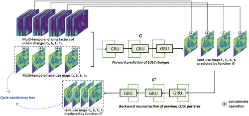
As illustrated in Figure 1, the proposed framework links two GRUs in a head-to-tail manner to form a cycle, in which one network is adopted for forwarding prediction and the other is for backward prediction. During the process of training, the output of the forward predictor $\mathit{G}$ becomes the input for the backward predictor $G^{\prime }$. To be more specific, LULC maps of time steps $t_0,t_1,\dots ,t_n$ and related multi-temporal predictor variables are concatenated as the input for function $\mathit{G}$, which maps the input to a prediction of the LULC maps of the time step $t_1,t_2,\dots ,t_{\mathit{n}+1}$. Then the predicted LULC maps are concatenated with driving factors $t_0,t_1,\dots ,t_n$ as the input for function $G^{\prime }$, which maps its input back to the estimated LULC maps of time steps $t_0,t_1,\dots ,t_n$. The equations of a GRU layer can be expressed as follows:

Figure 1. The overview of the structure of the proposed method, Cycle-Gated Recurrent Unit (GRU), which implements cycle-consistent learning on two GRU networks: one GRU for forward prediction and the other for backward prediction.

(1) $z_t=\mathit{\hspace{0.17em}}\mathit{\sigma }\left(W_{\mathit{xz}}{\mathrm{X}}_t+W_{\mathit{hz}\mathit{\hspace{0.17em}}}{\mathrm{H}}_{\mathit{t}-1}+\mathit{\hspace{0.17em}}{\mathrm{b}}_z\right)$(1)

(2) $r_t=\mathit{\hspace{0.17em}}\mathit{\sigma }\left(W_{\mathit{xr}}{\mathrm{X}}_t\mathit{\hspace{0.17em}}+W_{\mathit{hr}\mathit{\hspace{0.17em}}}{\mathrm{H}}_{\mathit{t}-1}\mathit{\hspace{0.17em}}+\mathit{\hspace{0.17em}}+{\mathrm{b}}_r\right)$(2)

(3) ${\hat{H}}_{\mathit{t}}=\mathit{\hspace{0.17em}}\mathit{tanh}\left(W_{\mathit{xh}}{\mathrm{X}}_t\mathit{\hspace{0.17em}}+W_{\mathit{hh}\mathit{\hspace{0.17em}}}\left(r_t\mathit{\hspace{0.17em}}\circ \mathit{\hspace{0.17em}}{\mathrm{H}}_{\mathit{t}-1}\right)\mathit{\hspace{0.17em}}+{\mathrm{b}}_h\right)$(3)

(4) ${\mathrm{H}}_t=\left(1-z_t\right)\circ \mathit{\hspace{0.17em}}{\mathrm{H}}_{\mathit{t}-1}+\mathit{\hspace{0.17em}}{z}_t\circ \mathit{\hspace{0.17em}}{\hat{H}}_{\mathit{t}}$(4)

where $z_t$ denotes an update gate at time step $\mathit{t}$, $r_t$ denotes a reset gate at time step $\mathit{t}$. ${\hat{H}}_{\mathit{t}}$, ${\mathrm{H}}_{\mathit{t}-1}$, ${\mathrm{H}}_t$ denotes a candidate memory state, a previous memory state, and a memory state for output of time step $\mathit{t}$, respectively. ${\mathrm{X}}_t$ denotes the input data at time step $\mathit{t}$. $\mathit{W}$ and $\mathit{b}$ refer to weight matrix and bias. $\mathit{\sigma }$ is the Sigmoid activation function, $\mathit{tanh}$ is the tangent function, and ∘ refers to element-wise multiplication.

Regarding the loss function, the loss of the predictor $L_{\mathit{pred}}$ and the cycle-consistency loss $L_{\mathit{cyc}}$ are calculated using the cross-entropy loss function. We express the objective as:

(5) $L_{\mathit{pred}}\left(\mathrm{G}\right)=\mathit{\hspace{0.17em}}-\sum _{\mathit{c}=1}^C{Y}_c\mathrm{logG}\left({\mathrm{X}}_c\right)$(5)

(6) $L_{\mathit{cyc}}\left(\mathrm{G},{\mathrm{G}}^{\prime }\right)=\mathit{\hspace{0.17em}}-\sum _{\mathit{c}=1}^C{\mathrm{X}}_c\log {\mathrm{G}}^{\prime }\left(\mathrm{G}\left({\mathrm{X}}_c\right)\right)$(6)

where ${\mathrm{X}}_c$ is the input data, $Y_c$ is the target data, and $\mathit{c}$ denotes the number of classes. The total loss is the sum of the loss of the predictor $L_{\mathit{pred}}$ and the cycle-consistency loss $L_{\mathit{cyc}}$. Thus, the loss of the whole framework $\mathit{L}$ can be expressed as:

(7) $\mathit{L}\left(\mathrm{G},\mathrm{G}{ }^{\mathrm{\prime }}\right)=\mathit{\hspace{0.17em}}{L}_{\mathit{pred}}\left(\mathrm{G}\right)+L_{\mathit{cyc}}\left({\mathrm{G}}^{\prime }\right)$(7)

Thus, the model computes the total loss $\mathit{L}$ after iteration, this total loss assesses the model performance in predicting future LULC patterns and its ability to reconstruct the original input. The total loss $\mathit{L}$ is then used in backpropagation, a method where the error is propagated back through the network, leading to an adjustment of the model’s weights and biases. These adjustments are informed by optimization algorithms and aim to minimize the loss in the next iteration.

2.2. Local surrogate method for interpreting individual predictions

The study uniquely adopted a local surrogate for interpreting individual predictions of LULC changes, which would be produced by the proposed deep recurrent network, Cycle-GRU. We follow the logic of LIME (Ribeiro, Singh, and Guestrin 2016) to develop a local surrogate method in a scenario of LULC prediction. The objective of applying the local surrogate model in this study is to extract understandable patterns and significant predictors, using logistic regression models as a form of the local surrogate model to approximate local decision boundaries around a specific point or region in the input space. This approach enables the estimation of the feature importance of input variables for predicted urban land changes.

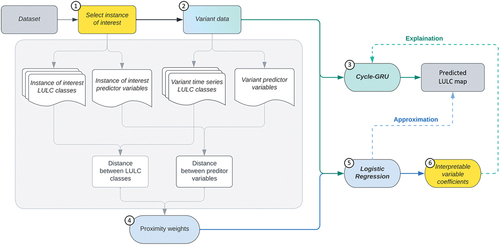
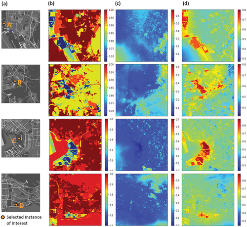
As shown in Figure 2, in this study, the process of training a local surrogate model can be divided into the following steps (Molnar 2022): (1) select an instance of interest: This is a data point within a selected subset of the study area, whose prediction is sought to be explained; (2) collect variant data: variant data refers to additional data points within the selected subset of the study area. Given that the remaining data points in the study area feature geographical proximity to the instance of interest, they share certain similar characteristics, such as road density and housing price. Therefore, it is anticipated that the variant data can be used to reflect the local behavior of the complex model when making predictions about the instance of interest; (3) generate predictions of the variant data using the trained deep learning model; (4) compute proximity weights: proximity weights are used to indicate the relevance or similarity between the instance of interest and the variant data. This ensures that the surrogate model prioritizes those instances that are closer or more similar to the instance for which an explanation is sought; (5) train the surrogate model: train a weighted logistic regression model on the variant data, where each data point is weighted by its proximity weight to approximate the local decision boundary of the deep learning model; (6) model interpretation: the coefficients of the trained logistic regression model indicate the importance of each feature in predicting the instance of interest within the local area defined by the variant data; (7) compute fidelity score: measure how accurately the predictions of the surrogate model match the predictions of the deep learning model it is approximating.

Figure 2. The framework of the proposed local surrogate method for interpreting urban expansion predictions. The framework consists of six steps: (1) selection of an instance of interest; (2) variant data collection; (3) generation of predictions using variant data; (4) generation of proximity weights; (5) training of the surrogate model; and (6) interpretation of coefficients.

To interpret the prediction of instance $\mathrm{x}$, the objective of surrogate model $\mathit{s}$ is to (i) minimize the distance between the predicted results of the deep learning model $\mathit{G}$ and the prediction of the surrogate model $\mathit{s}$, and (ii) maintain a low level of model complexity of the surrogate model $\mathit{s}$. The explanation $\mathit{\xi }\left(\mathrm{x}\right)$ of the local surrogate model can be yielded as follows (Ribeiro, Singh, and Guestrin 2016):

(8) $\mathit{\xi }\left(\mathrm{x}\right)=\arg \underset{\mathit{s}\in \mathit{S}}{min}\mathit{L}\left(\mathit{G},\mathit{s},{\pi }_x\right)+\mathrm{\Omega }\left(\mathit{s}\right)$(8)

where S denotes all possible explanations. $\mathrm{\Omega }\left(\mathit{s}\right)$ measures the model complexity, which should be at a low level of complexity that can enable interpretation. ${\pi }_x$ is an exponential kernel which produces proximity weights of data samples for training a surrogate model, the proximity weights are generated based on the distance between instance $\mathit{x}$ and variant data $\mathit{x}{ }^{\mathrm{\prime }}$. The function for computing proximity weights is the radial-basis function (RBF) kernel, also known as the square-exponential kernel, which can be expressed as:

(9) ${\pi }_x=\mathit{k}\left(\mathit{x},\mathit{\hspace{0.17em}}\mathit{x}{ }^{\mathrm{\prime }}\right)=\exp \left(-\frac{{\left(\mathit{d}\left(\mathit{x},\mathit{\hspace{0.17em}}x{\mathit{ }}^{\mathrm{\prime }}\right)\right)}^2}{2l^2}\right)$(9)

where $\mathit{l}$ is the length scale of the kernel, $\mathit{d}$ measures the distance between the instance $\mathrm{x}$ and variant data $\mathit{x}{ }^{\mathrm{\prime }}$.

It should be noted that, the input data contains both discrete variables (i.e. land use and land cover classes) and continuous variables (e.g. slope, DEM). Thus, the distance $\mathit{d}$ between the instance $\mathrm{x}$ and variant data $\mathit{x}{ }^{\mathrm{\prime }}$ should be computed with suitable functions according to data types. Specifically, the distance between the discrete variables of the selected instance $x_d$ and the discrete variables of the variant data $x_d^{\prime }$ are computed by the Jaccard coefficient method, which measures the similarity between finite data sets. The distance between the continuous variables of the selected instance $x_c$ and the continuous variables of the variant data $x_c^{\prime }$ are computed by Euclidean distance.

(10) $d_{\mathit{Jcarrd}}\left(x_d,x_d^{\prime }\right)=1-\frac{\left|x_d\cap x_d^{\prime }\right|}{\left|x_d\cup x_d^{\prime }\right|}$(10)

(11) $d_{\mathit{euclidean}}\left(x_c,\mathit{\hspace{0.17em}}{x}_c^{\prime }\right)=\left|x_c-\mathit{\hspace{0.17em}}{x}_c^{\prime }\right|$(11)

(12) $\mathit{d}\left(\mathit{x},\mathit{\hspace{0.17em}}\mathit{x}{ }^{\mathrm{\prime }}\right)=d_{\mathit{Jcarrd}}\left(x_d,\mathit{\hspace{0.17em}}{x}_d^{\prime }\right)+d_{\mathit{euclidean}}\left(x_c,\mathit{\hspace{0.17em}}{x}_c^{\prime }\right)$(12)

A logistic regression model is selected as the local surrogate model to interpret prediction instances produced by a trained Cycle-GRU model. A logistic regression model can be regarded as a single-layer neural network, in which the weights and variables are computed with a linear function and then activated through a non-linear function (Bishop and Hinton 1995). One of the advantages of logistic regression is that it can effectively analyze relationships among variables (Ayer et al. 2010; Müller and Mburu 2009). More importantly, logistic regression is capable of ranking the importance of variables through the process of training models (Dreiseitl and Ohno-Machado 2002), the importance of each input variable can be indicated by its corresponding coefficient weight (Kim et al. 2017). With the generated proximity weights ${\pi }_x$, a logistic regression model can be trained to approximate the prediction of a Cycle-GRU. Then the coefficient of the trained logistic regression model can be extracted to identify the influence of predictor variables on individual predictions. Existing studies on temporal importance suggest that the preceding time step of the prediction target is the most crucial time step throughout the entire input time series. For instance, a spatial-temporal attention mechanism was implemented, revealing that the last time stamp of the input sequence holds the greatest significance for predicting the subsequent step (Liu, Zhou, and He 2019). Also, a temporal attention mechanism was applied to a temporal convolutional network, suggesting that the model predominantly relies on the last input steps for the prediction (Pantiskas, Verstoep, and Bal 2020). Therefore, considering that the logistic regression model is not a multi-temporal model, we trained multiple logistic regression models to approximate each time stamp and then averaged the weights of all the input features over the entire temporal sequence.

3. Dataset and experiment setup

3.1. Dataset

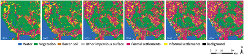
The study case is Shenzhen, a coastal city located in southern China. Shenzhen has witnessed an unprecedented rate of urban expansion over the last four decades, it shifted from an agricultural-dominant landscape to a rapid urbanization landscape since the late 1970s (W. Li et al. 2005). The study area of this work has a spatial coverage of 1,296 square kilometers. The dataset consists of two types of data, (1) multi-temporal LULC maps and (2) land change driving factors. The LULC maps contain six land use classes, including water, vegetation, barren soil, formal settlements, informal settlements, and other impervious surfaces. The class of informal settlements refers to the prevalent urban villages in the study area. The class of other impervious surfaces includes road networks and other impervious pavements.

As shown in Figure 3, the dataset contains six time steps from 1995 to 2020 with an interval of around five years. The multi-temporal LULC maps were derived from Landsat images and generated by a U-Net-ConvLSTM model with a post-classification relearning strategy (Geiß et al. 2020; Zhu et al. 2021), and the classification accuracy reaches 84.9% on a validation dataset. Then, these multi-temporal LULC maps were manually enhanced according to available historic Google Earth images for further calibration. It should be noted that, since the time-series LULC maps adopted in this study have a temporal resolution of a five-year interval, models trained based on this temporal resolution are aimed at providing insights into urban expansion for the subsequent time step, also occurring at a five-year interval.

Figure 3. Land use and land cover maps of the study area for urban expansion prediction. The dataset contains six time steps from 1995 to 2020, with five-year intervals.

The predictor variables adopted in existing studies of LULC prediction can mainly be divided into four categories, which are (i) environmental variables (e.g. waterbody, terrain, soil, climate) (Liu et al. 2017; Mu et al. 2019; Pijanowski et al. 2002; Singh 2017; Wang et al. 2018), (ii) infrastructure variables (e.g. roads, transport stations, POIs) (Pijanowski et al. 2002; Wang et al. 2018; Zhang 2016), (iii) land use-related variables (e.g. agriculture, vegetation, built-up) (Liu et al. 2017; Mu et al. 2019; Pijanowski et al. 2002; Shafizadeh-Moghadam, Tayyebi, and Helbich 2017; Zhang 2016), and (iv) social-economic variables (e.g. population, housing prices) (Gómez et al. 2020; Liu et al. 2017; Mu et al. 2019; Singh 2017). Among these four types of predictor variables, distance-based predictor variables are a commonly adopted type of data, which carry continuous statistics of positional information, such as distance to roads (Liu et al. 2017; Pijanowski et al. 2002; Singh 2017; Zhang 2016) and distance to water bodies (Pijanowski et al. 2002; Shafizadeh-Moghadam, Tayyebi, and Helbich 2017; Wang et al. 2018). It is worth mentioning that distance to roads and distance to built-up areas (Mu et al. 2019; Pijanowski et al. 2002, 2014; Shafizadeh-Moghadam, Tayyebi, and Helbich 2017; Zhang 2016) are two major types of predictor variables with various variants. Environmental variables and infrastructural variables are also large groups that contain many variants. In addition, economic variables, such as housing prices, have not been extensively adopted in existing studies.

Table 1. Summary of the information on the 19 predictor variables adopted for urban expansion prediction in this study.

	Variables		Temporal resolution	Spatial resolution
1	LULC maps	LULC maps: water	1995\2000\2005\2010\2015\2020	30 m
2		LULC maps: vegetation	1995\2000\2005\2010\2015\2021	30 m
3		LULC maps: barren soil	1995\2000\2005\2010\2015\2022	30 m
4		LULC maps: other impervious surfaces	1995\2000\2005\2010\2015\2023	30 m
5		LULC maps: formal settlements	1995\2000\2005\2010\2015\2024	30 m
6		LULC maps: informal settlements	1995\2000\2005\2010\2015\2025	30 m
7	Housing price		1995\2000\2005\2010\2015\2021	District level (interpolate to 30 m)
8	Accessibility of metro stations		2004/2010/2015/2020	30 m
9	DEM		static	30 m
10	Policy factors: proximity to Special Economic Zone (SEZ) and CBD		before 2010/after 2010	30 m
11	Slope		static	30 m
12	Solar radiation (the whole year with one month interval)		static	30 m
13	Distance to roads	Distance to roads: primary road	1995\2000\2005\2010\2015\2020	30 m
14		Distance to roads: secondary road	1995\2000\2005\2010\2015\2020	30 m
15		Distance to roads: tertiary road	1995\2000\2005\2010\2015\2020	30 m
16		Distance to roads: motorway	1995\2000\2005\2010\2015\2020	30 m
17		Distance to roads: nonmotorized vehicle lane	1995\2000\2005\2010\2015\2020	30 m
18	Distance to urban extents		1995\2000\2005\2010\2015\2020	30 m
19	Distance to formal settlements		1995\2000\2005\2010\2015\2020	30 m

As one of the advantages of ML in simulating land change is that it can involve all driving forces in the modeling process (Aburas, Ahamad, and Omar 2019), we collected all available data of the study area. In total, eight categories of land change predictor variables were collected as input variables for LULC change prediction (Table 1), including (1) housing price, (2) distance to metro stations, (3) Digital Elevation Maps (DEM), (4) proximity to CBD, (5) slope, (6) solar radiation, (7) distance to road networks, and (8) distance to built-up areas. The DEM data, with a spatial resolution of 30 meters, was sourced from ASTER DEM and used to generate slope and solar radiation maps. The solar radiation map was created using ArcGIS, with calculations made for the entire year at half-hour intervals on a fortnightly basis. Housing price data from 2000 to 2020 was obtained from the Shenzhen Statistical Yearbook. To convert district-level housing price data to raster maps, kriging interpolation was employed. Data on metro stations were sampled according to initial service times and classified into four types based on the number of connected metro lines. Distance to each type of metro station was computed using the Euclidean distance function. Multi-temporal distance maps to SEZ and CBD were calculated using Euclidean distance functions based on SEZ locations and Futian CBD coverage and changes. Road network data was extracted from OpenStreetMap (OSM) and simplified into five road types. Historical road network data was manually adjusted based on corresponding satellite images. Distances to road types were calculated using the Euclidean distance function. Distance to urban extents included two layers: distance to all settlements and distance to urban settlements excluding urban villages. Urban extent data was extracted from classified LULC maps and computed using the Euclidean distance function. All predictor variables were standardized, with a mean of zero and a standard deviation of one, and combined with pre-processed land use maps as input for the models. As shown in Table 1, in total, 19 variables were adopted for the prediction of urban expansion in this study.

The recurrent connections in GRU and LSTM cells allow them to model long-term dependencies in sequential data. They capture temporal patterns by selectively incorporating important information from each time step while updating the hidden states over time. However, GRU and LSTM are generally not well-suited for explicitly capturing spatial correlations in data. To compensate for the lack of spatial structure in GRU and LSTM, we converted key spatial features, such as the distance to road networks and urban centers, into numeric values and used them as input variables for model training. In this manner, the models are anticipated to be more focused on extracting significant temporal dependencies in the data, which emphasizes the learning of the transition rules embedded in the dataset.

3.2. Experiment setup

The experiment of the proposed prediction method can be divided into two stages: (i) train a deep learning model for LULC prediction; (ii) train a local surrogate model for interpreting individual predictions produced by the deep learning model.

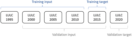
For the test in the first stage, the multi-temporal dataset was split into a training dataset and a validation dataset along the temporal dimension (Figure 4). The training dataset contains the first five steps (1995–2015), whereas the validation dataset consists of the last five steps (2000–2020). In both training and validation datasets, the variables of the first four time steps were adopted as input and the last time step was used as the ground truth labels. As such, the target of the training dataset is to predict the LULC map for the year 2015, and the goal of the validation dataset is to project the LULC pattern for the year 2020. The size of each variable in spatial dimension is 1,200 by 1,200 pixels. For training and validation, the training dataset was spatially subsampled into 80 pieces of cropped images with a size of 256 by 256 pixels, and the validation was conducted on the entire spatial coverage of the predicted LULC map of the year 2020. To evaluate the proposed methods, four baseline methods were adopted, including a multi-layer perception model (MLP) (Pijanowski et al. 2002), a vanilla CNN model, an LSTM model, and a GRU model. The rationale for the selection of baseline models is focused on evaluating different data processing capabilities. The MLP offers a basic data handling benchmark, while the CNN addresses spatial data processing of urban patterns without taking into account sequential relationships. LSTM and GRU are chosen for their sequential data processing ability. Given the lack of consensus on the superiority between LSTM and GRU, both are used as foundational models to apply cycle-consistent learning. This approach allows for a nuanced evaluation of how advanced techniques augment the ability to process the patterns of urban dynamics, comparing them against established spatial and sequential data processing methods.

Figure 4. An overview of the experimental setup for urban expansion prediction. The dataset is split into a training dataset and a validation dataset along the temporal dimension, with each dataset containing five time steps.

Then the proposed framework, cycle consistency, was applied to both LSTM and GRU models for comparison. The recurrent methods with the cycle consistency mechanism are named Cycle-GRU and Cycle-LSTM. Standard GRU and LSTM are employed as the backbone model. The input size of the Cycle-GRU and Cycle-LSTM is 19, corresponding to the number of predictor variables adopted in this study. Both Cycle-GRU and Cycle-LSTM have two hidden layers, which feature a hidden size of 32 and 16 respectively. In total six different methods were tested in this study. The deep learning models in this study were tested with PyTorch on an NVIDIA GeForce RTX 3090. All the tested models were trained for 150 epochs with a batch size of 4, the optimizer was Adam, and the learning rate was set to 8 × 10^-4. The learning rate decreases to a fraction of 0.8 when the training accuracy stops decreasing for 10 epochs. All the models were evaluated over 150 epochs according to the best estimated generalization capability. The loss function for baseline methods is cross-entropy loss.

The evaluation methods for assessing model performance include overall pixel accuracy (OA), kappa indices (i.e. Kappa coefficient, K location, K histogram), Recall, Precision, F1 scores, and Quantity Disagreement and Allocation Disagreement (QDAD) (Pontius and Millones 2011). These evaluation metrics have been widely adopted in studies of land change prediction, assessing model performance from different perspectives (Chaudhuri and Clarke 2014; Liu et al. 2017; Qian et al. 2020; Wu et al. 2022; Xing et al. 2020). In particular, OA offers a basic measure of the correctly predicted pixels. Kappa indices are computed based on the confusion matrix generated by a pixel-by-pixel categorical comparison of the simulation and the ground truth. K location emphasizes location disagreement while K histogram is more sensitive to quantitative similarity. Recall, Precision, and F1 scores are based on the calculation of true positives, true negatives, false positives, and false negatives. Given that urban expansion simulations often feature a significant number of unchanged pixels, it is advisable to concentrate evaluations on the changed pixels. In this respect, QDAD analysis enhances the evaluation process by breaking down prediction errors into categories of misallocation and inaccurate quantity estimates, thus providing a thorough evaluation of model performance.

In the second stage, instances were selected from the validation dataset for the test of local surrogate models. The input data of an instance contains various attributes of the pixel in the dataset. For each instance, a neighboring area of 256 by 256 pixels is employed as the variant data for training a local surrogate model. In total, four instances were selected to test the feasibility of adopting a local surrogate approach for interpreting land change predictions generated by a deep learning model. As aforementioned, the local surrogate model trained for interpreting a Cycle-GRU model is a logistic regression model, which was established with the Scikit-learn library. Since logistic regression models cannot handle multi-temporal data, we adopted the data from each time step as the training input to approximate the predictions of the subsequent year generated by the trained Cycle-GRU model. Then, the weights of all trained logistic regression models were averaged to determine the feature importance over the entire temporal sequence. The local fidelity scores were evaluated using overall pixel accuracy by comparing the predictions of logistic regression models to corresponding predictions of the trained Cycle-GRU. At last, the coefficients of the trained logistic regression models were extracted to indicate the influence of input variables on individual predictions of the Cycle-GRU model. Additionally, SHAP method was also adopted to provide supplementary information on the influence of variables on model predictions.

4. Results and discussions

4.1. Evaluation of the prediction performance

The OA, kappa indices, Recall, Precision, and F1 scores of all the tested DNNs are shown in Figure 5. As can be observed, the proposed method, Cycle-GRU, allowed the best overall performance in terms of OA and kappa indices. Since the task of LULC prediction is associated with time-series data, the DNNs that do not consider the temporal dependency in the data (i.e. MLP and CNN) generally yield poor performance. In contrast, recurrent models achieved substantially better performance. In particular, Cycle-GRU presented the best overall performance among all the tested methods with 93.1% OA and 90.2% kappa coefficient. Also, Cycle-LSTM achieved a very competitive performance compared to Cycle-GRU with 93.0% OA and the same kappa coefficient as Cycle-GRU. Regarding the performance of tested models in Recall, Precision, and F1 scores, Cycle-LSTM and Cycle-GRU showed the best and the second-best scores among all the tested models.

Figure 5. Comparison of experimental results for the proposed methods and baseline methods, evaluated using a series of metrics, including overall pixel accuracy (OA), Kappa indices, Recall, Precision, and F1 score.

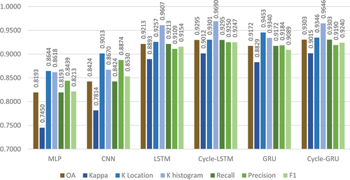
It can be detected that the mechanism of cycle consistency brought substantial performance gains in both LSTM-based and GRU-based methods. For instance, the OA of LSTM increased from 92.1% to 93.0%, and the OA of GRU improved from 91.7% to 93.1%. Moreover, the cycle mechanism also exhibited beneficial effects on the patterns of K statistics. After the implementation of the cycle mechanism, the kappa coefficient of LSTM improved from 0.889 to 0.902, and the kappa coefficient of GRU increased from 0.883 to 0.902. Besides, the patterns of K statistics were also improved after the incorporation of the cycle mechanism. For instance, the K Location and K Histogram indices for Cycle-GRU indicate a robust model with a heightened ability to predict the overall quantity of land classes with high precision, evidenced by a substantially higher K Histogram score of 0.965 compared to that of the GRU. Additionally, it maintained precision in mapping the spatial distribution of land classes, achieving a score of 0.935 in K Location. The effect can also be observed in Recall, Precision, and F1 scores, both Cycle-LSTM and Cycle-GRU showed significant increases in these metrics compared to their counterpart methods.

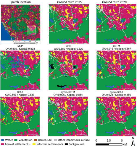
Subsets of predicted results generated by tested methods are visualized for comparison. The validation subset is an area in the southeast part of the study area, the specific location of the subset was highlighted with a square in the first diagram in Figure 6, and the ground truth of the prediction result of the subset is also presented in Figure 6 for comparison. As can be observed, the LULC maps predicted by MLP and CNN exhibit significant errors. In particular, the prediction of MLP contains a large area of false prediction in water coverage, and the result of CNN presents limited predictive capability in terms of forecasting the land transitions from barren soil to built-up areas. In contrast, the performance gains introduced by the cycle consistency can be visually detected in the predicted results of Cycle-LSTM and Cycle-GRU. In particular, Cycle-LSTM presented better performance than vanilla LSTM in terms of anticipating the changes in informal settlements, the false positive prediction of informal settlements is alleviated in the results of Cycle-LSTM. Also, the result of vanilla GRU falsely predicted road networks as informal settlements, these mistakes were significantly corrected in the result of Cycle-GRU.

Figure 6. Comparison of the predicted results of a validation subset generated by all the tested methods. Information on overall pixel accuracy (OA) and Kappa coefficient is provided. The location of the subset in the study area is highlighted in the first subplot.

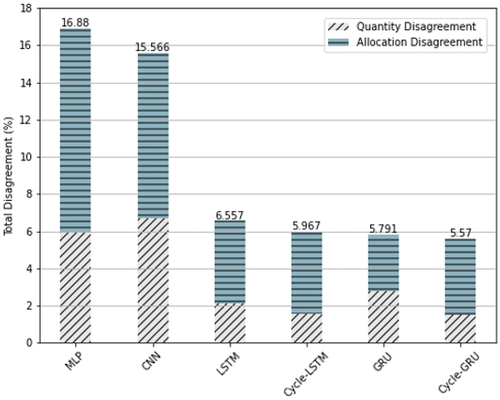
The evaluation of QDAD between the predicted urban area and the ground truth is presented in Figure 7. Among all the tested methods, Cycle-GRU yielded the smallest overall disagreement regarding the prediction of urban expansion. Also, the results of QDAD suggest that the implementation of the cycle mechanism brought substantial improvements to the two recurrent neural network methods tested in this study. Specifically, the QDAD values of vanilla LSTM and GRU dropped from 6.557% and 5.791% to 5.967% and 5.570% respectively. Regarding the performance of Cycle-LSTM and Cycle-GRU, although Cycle-LSTM yielded higher scores in Precision and F1 scores, Cycle-GRU achieved the best scores in Kappa indices and QDAD, indicating a better performance in predicting the expanded urban extent.

Figure 7. The evaluation results of Quantity Disagreement and Allocation Disagreement (QDAD) of the predicted urban expansion by all the tested methods.

4.2. Interpretation with local surrogate models

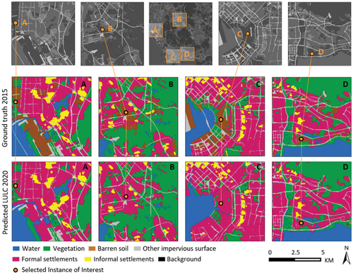
Four instances were selected for testing the approach of adopting local surrogate models to interpret individual predictions of urban expansion. The four selected instances are situated in four different locations in the study area, highlighted with yellow dots. As illustrated in Figure 8, two of the instances are located in the city center areas C and D, and the other two instances are located in the suburban areas A and B. All of the selected instances were cells that were barren soil in 2015 and predicted to transit to formal settlements in 2020. The remainder cells in these four selected subsets of the study area were employed as the variant data for the four instances of interest, respectively.

Figure 8. The locations and land use changes of four selected instances for testing the proposed local surrogate method. Instances a and B are in suburban areas, instances C and D are located in the city center. The four instances were barren soil in 2015 and were predicted to be formal settlements in 2020.

Following the equations introduced in Section 2.2, for each selected instance, the proximity weights of its corresponding variant data were computed according to their similarity with the selected instance. As shown in Figure 9, the distance of LULC classes and the distance of predictor variables were calculated with Equations 10(10) $d_{\mathit{Jcarrd}}\left(x_d,x_d^{\prime }\right)=1-\frac{\left|x_d\cap x_d^{\prime }\right|}{\left|x_d\cup x_d^{\prime }\right|}$(10) and 11(11) $d_{\mathit{euclidean}}\left(x_c,\mathit{\hspace{0.17em}}{x}_c^{\prime }\right)=\left|x_c-\mathit{\hspace{0.17em}}{x}_c^{\prime }\right|$(11) , respectively. The sum of the LULC distance and predictor variable distance was further computed for the generation of proximity weights of each subset. Then local surrogate models were trained with the variant data of each instance, as well as the corresponding proximity weights. As a result, the local fidelity score of the local surrogate model trained for area A is 98.60%, area B is 99.11%, area C is 98.17%, and area D is 98.58%.

Figure 9. The generation of proximity weights is based on the similarity between the instances of interest and their variant data, which is computed based on the values of predictor variables: (a) the location of the selected instance of interest; (b) the distances to land cover variables; (c) the distances to other predictor variables; and (d) the generated proximity weights.

The coefficients of the trained local surrogate models that can indicate the relationships between input variables and predictions are normalized and presented in Figure 10. As can be observed, the distributions of coefficients for all four local explainers presented similar patterns. For the interpretation of all the selected instances, LULC variables generally yielded the largest magnitude coefficients for the prediction of LULC changes in the next time step. This finding aligns with existing studies suggesting that urban land changes are highly correlated with historical land change trends (Gidey et al. 2017). Specifically, previous formal settlements (e.g. +0.49 in area A, +0.53 for area B) and barren soil (e.g. +0.56 in area A, +0.49 for area B) are the most significant features for predicting urban expansion. This also corresponds to the predictions of the Cycle-GRU at the selected instances of interest, where barren soil cells were forecasted to convert into formal settlements. The variable of distance to built-up areas presents a substantially negative influence on the prediction of formal settlements in all the trained local surrogate models (e.g. −0.34 for area A, −0.35 for area B). In addition, previous vegetation land (e.g. −0.27 for area A, −0.33 for area B) and water bodies (e.g. −0.33 for area A, −0.30 for area B) exhibit considerably negative relationships with the prediction of formal settlements. Transportation factors are often included in studies of urban dynamics due to their influence on the process of land transitions (Gidey et al. 2017; Iacono and Levinson 2009; Poelmans and Van Rompaey 2010; Wu et al. 2022). In this study, most of the distance to road variables tend to feature a negative influence with the prediction of formal settlements (e.g. −0.13 for primary roads in area A, −0.20 for tertiary roads in area C) and informal settlements (e.g. −0.27 and −0.15 for secondary roads in area C and D, respectively). This is consistent with the findings that while transportation variables can affect land use changes, their impact is less pronounced than that of variables representing existing land use patterns (Iacono and Levinson 2009).

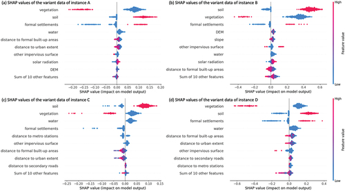
Figure 10. SHapley Additive exPlanations (SHAP) values of Cycle-Gated Recurrent Unit (GRU) models for predicting formal settlements with the variant data of the four selected instances of interest: (a) variant data of instance A; (b) variant data of instance B; (c) variant data of instance C; and (d) variant data of instance D.

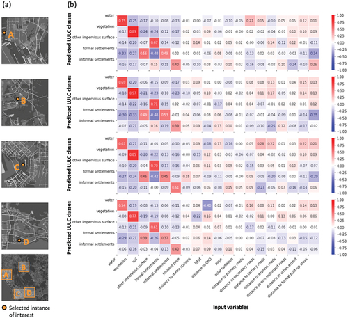
There are also some disagreements between the coefficient distribution in urban and suburban areas. As shown in Figure 10, the prediction of formal settlement and informal settlement presented almost contrary patterns in terms of their relationship with the variables of proximity to CBD and distance to primary roads. In particular, the proximity to CBD presented negative influences on the prediction of urban expansion of the city center instances (i.e. −0.11 for area C, −0.06 for area D), whereas the proximity to CBD showed positive influences on the prediction of urban expansion of the suburban instances (i.e. +0.08 for area A, +0.06 for area B). The coefficient distribution also indicated a divergence regarding the relationship between formal settlements and the distance to primary roads. The predicted formal settlements in suburban areas were negatively related to the distance to primary roads (i.e. −0.13 for area A, −0.07 for area B), indicating that as the distance decreases, the likelihood of formal settlements increases. Conversely, in city center areas, the predicted formal settlements were positively related to the distance to primary roads (i.e. +0.09 for area C), suggesting that formal settlements are more likely to occur farther from these roads. The differences in coefficient values of proximity to CBD and distance to primary roads in different urban areas can also be attributed to the changes in their roles in the dynamic process of urban expansion, with some development being less confined to traditional urban centers and more influenced by the accessibility provided by road networks (Poelmans and Van Rompaey 2010). This can be observed from the different expansion patterns in city centers and suburban areas, expansion in city centers is more likely to consist of infill within existing urban structures, while expansion in suburban areas tends to be dispersed and closely follows the layout of primary roads. By and large, the above-discussed agreements and disagreements between the coefficients of the four local surrogate models can be reasonably explained based on the characteristics of the data sets.

Additionally, the method of SHapley Additive exPlanations (SHAP) was adopted to provide complementary information on the interpretability of the trained model. Figure 11 presents the SHAP values of variables for predicting formal settlements in four selected areas. Overall, the implications of SHAP values align with the general distribution of variable coefficients generated by the proposed interpretation methods. Both methods indicate a strong correlation between some historic land use classes (i.e. vegetation, soil, and formal settlements) and the predicted urban expansion. This includes the positive impact of previous formal settlements and soil on model predictions and the negative impact of former vegetation on these predictions. The agreement between these two interpretation methods on the importance of key variables strengthens confidence in the proposed interpretation approach.

5. Conclusions

In this study, we proposed an interpretable deep learning approach tailored for the predictive modeling of urban land dynamics. Considering time series LULC data usually features a limited length of time frames, the proposed method is tailored for short-term time series data. We uniquely implemented the mechanism of cycle consistency on a GRU model to improve its capability of processing multi-temporal LULC data. In total, six different methods were tested and assessed with different evaluation metrics, including using both LSTM and GRU models as the backbone model in a cycle-consistency framework. As a result, a substantial level of performance gains can be observed in both LSTM and GRU methods after the implementation of the cycle mechanism, and a cycle-GRU showed the best overall performance in terms of prediction accuracy.

Figure 11. Coefficients of local surrogate models trained with the variant data of the selected instances of interest: (a) the location of the selected instances of interest: A and B in suburban areas, C and D in city center areas; (b) coefficients of each predictor variable for the prediction of each land cover class.

The study also investigated the feasibility of applying local surrogate models for interpreting the predicted instances of the proposed deep learning model. Four instances of predicted urban expansion were selected for interpretation tests. Correspondingly, four sets of local surrogate models were adopted as local explainers, which were trained with variant data and proximity weights. The experimental results confirmed the effectiveness of the local surrogate approach in terms of providing interpretable local explanations to identify the influence of predictor variables on individual predictions. Notably, since the interpretable mechanism is designed for local explainability, the coefficients of the trained local surrogate models showed similar patterns in general, whereas there are some varied patterns between instances, which can be linked with the attributes of their locations in the study area.

There are certain limitations to this study. First, the study only applied Shenzhen as the case study due to the availability of time series data collection. The generalizability of the proposed method needs to be tested in further studies. Secondly, the hyperparameters of the proposed method were selected based on the model’s performance on the study area’s data. It is anticipated that certain adaptations of hyperparameters may be required for specific tasks. For future research, the proposed method holds potential for application to various tasks involving time-series geospatial data processing. Further studies will also explore its generalizability across datasets from different geographic regions and assess the practical utility of the proposed framework in planning practices.

Disclosure statement

No potential conflict of interest was reported by the author(s).

Data availability statement

The data that support the findings of this study are available from the corresponding author, Y.Zhu, upon reasonable request.

References

- Aburas, M. M., M. S. S. Ahamad, and N. Q. Omar. 2019. “Spatio-Temporal Simulation and Prediction of Land-Use Change Using Conventional and Machine Learning Models: A Review.” Environmental Monitoring and Assessment 191 (4): 205. April. https://doi.org/10.1007/s10661-019-7330-6.
- Angel, S., J. Parent, D. L. Civco, A. Blei, and D. Potere. 2011. “The Dimensions of Global Urban Expansion: Estimates and Projections for All Countries, 2000–2050.” Progress in Planning 75 (2): 53–21. February. https://doi.org/10.1016/j.progress.2011.04.001.
- Ayer, T., J. Chhatwal, O. Alagoz, C. E. Kahn, R. W. Woods, and E. S. Burnside. 2010. “Comparison of Logistic Regression and Artificial Neural Network Models in Breast Cancer Risk Estimation.” RadioGraphics 30 (1): 13–22. January. https://doi.org/10.1148/rg.301095057.
- Bengio, Y., P. Simard, and P. Frasconi. 1994. “Learning Long-Term Dependencies with Gradient Descent Is Difficult.” IEEE Transactions on Neural Networks 5 (2): 157–166. March. https://doi.org/10.1109/72.279181.
- Bishop, C. M., and G. Hinton. 1995. “Neural Networks for Pattern Recognition.”
- Boulila, W., H. Ghandorh, M. A. Khan, F. Ahmed, and J. Ahmad. 2021. “A Novel CNN-LSTM-based Approach to Predict Urban Expansion.” Ecological Informatics 64:101325. September. https://doi.org/10.1016/j.ecoinf.2021.101325.
- Bren d’Amour, C., F. Reitsma, G. Baiocchi, S. Barthel, B. Güneralp, K.-H. Erb, H. Haberl, et al. 2017. “Future Urban Land Expansion and Implications for Global Croplands.” Proceedings of the National Academy of Sciences of the United States of America 114 (34): 8939–8944. August. https://doi.org/10.1073/pnas.1606036114.
- Cahuantzi, R., X. Chen, and S. Güttel. July, 2021. “‘A Comparison of LSTM and GRU Networks for Learning Symbolic sequences’.” arXiv: 2107.02248 [cs]. Accessed January 17, 2022. [Online]. Available: http://arxiv.org/abs/2107.02248.
- Cao, C., S. Dragićević, and S. Li. 2019. “Short-Term Forecasting of Land Use Change Using Recurrent Neural Network Models.” Sustainability 11 (19, Art. no. 19): 5376. January. https://doi.org/10.3390/su11195376.
- Castelluccio, M., G. Poggi, C. Sansone, and L. Verdoliva. August, 2015. “Land Use Classification in Remote Sensing Images by Convolutional Neural Networks.” arXiv: 1508.00092 [cs]. Accessed April 23, 2019. [Online]. Available: http://arxiv.org/abs/1508.00092.
- Chaudhuri, G., and K. Clarke. 2014. “Temporal Accuracy in Urban Growth Forecasting: A Study Using the SLEUTH Model.” Transactions in GIS 18 (2): 302–320. https://doi.org/10.1111/tgis.12047.
- Cho, K., B. Merrienboer, D. Bahdanau, and Y. Bengio. 2014. On the Properties of Neural Machine Translation: Encoder-Decoder Approaches. September. https://doi.org/10.3115/v1/W14-4012.
- Chung, J., C. Gulcehre, K. Cho, and Y. Bengio. December., 2014. “‘Empirical Evaluation of Gated Recurrent Neural Networks on Sequence Modeling’.” arXiv: 1412.3555 [cs]. Accessed December. 8, 2021. [Online]. Available: http://arxiv.org/abs/1412.3555.
- Dewan, A. M., and Y. Yamaguchi. 2008. “Using Remote Sensing and GIS to Detect and Monitor Land Use and Land Cover Change in Dhaka Metropolitan of Bangladesh During 1960–2005.” Environmental Monitoring and Assessment 150 (1): 237. March. https://doi.org/10.1007/s10661-008-0226-5.
- Dong, X., W. Li, X. Wang, and Y. Wang. 2020. “Cycle-CNN for Colorization Towards Real Monochrome-Color Camera Systems.” Proceedings of the AAAI Conference on Artificial Intelligence 34 (7, Art. no. 07): 10721–10728. April. https://doi.org/10.1609/aaai.v34i07.6700.
- Dreiseitl, S., and L. Ohno-Machado. 2002. “Logistic Regression and Artificial Neural Network Classification Models: A Methodology Review.” Journal of Biomedical Informatics 35 (5–6): 352–359. October. https://doi.org/10.1016/S1532-0464(03)00034-0.
- Frosst, N., and G. Hinton. November, 2017. “Distilling a Neural Network into a Soft Decision Tree.” arXiv, arXiv: 1711.09784. https://doi.org/10.48550/arXiv.1711.09784.
- Gao, J., and B. C. O’Neill. 2020. “Mapping Global Urban Land for the 21st Century with Data-Driven Simulations and Shared Socioeconomic Pathways.” Nature Communications 11 (1, Art. no. 1). May. https://doi.org/10.1038/s41467-020-15788-7.
- Geiß, C., M. Jilge, T. Lakes, and H. Taubenböck. 2016. “Estimation of Seismic Vulnerability Levels of Urban Structures with Multisensor Remote Sensing.” IEEE Journal of Selected Topics in Applied Earth Observations and Remote Sensing 9 (5): 1913–1936. May. https://doi.org/10.1109/JSTARS.2015.2442584.
- Geiß, C., Y. Zhu, C. Qiu, L. Mou, X. X. Zhu, and H. Taubenböck. 2020. “Deep Relearning in the Geospatial Domain for Semantic Remote Sensing Image Segmentation.” IEEE Geoscience and Remote Sensing Letters, 1–5. https://doi.org/10.1109/LGRS.2020.3031339.
- Gidey, E., O. Dikinya, R. Sebego, E. Segosebe, and A. Zenebe. 2017. “Cellular Automata and Markov Chain (Ca_Markov) Model-Based Predictions of Future Land Use and Land Cover Scenarios (2015–2033) in Raya, Northern Ethiopia.” Modeling Earth Systems and Environment 3 (4): 1245–1262. December. https://doi.org/10.1007/s40808-017-0397-6.
- Gómez, J. A., J. E. Patiño, J. C. Duque, and S. Passos. 2020. “Spatiotemporal Modeling of Urban Growth Using Machine Learning.” Remote Sensing 12 (1, Art. no. 1): 109. January. https://doi.org/10.3390/rs12010109.
- Guidotti, R., A. Monreale, S. Ruggieri, D. Pedreschi, F. Turini, and F. Giannotti. 2018. “Local Rule-Based Explanations of Black Box Decision Systems.” arXiv Preprint arXiv: 150302531 2. May 28. https://doi.org/10.48550/arXiv.1805.10820.
- Haregeweyn, N., G. Fikadu, A. Tsunekawa, M. Tsubo, and D. T. Meshesha. 2012. “The Dynamics of Urban Expansion and Its Impacts on Land Use/Land Cover Change and Small-Scale Farmers Living Near the Urban Fringe: A Case Study of Bahir Dar, Ethiopia.” Landscape and Urban Planning 106 (2): 149–157. May. https://doi.org/10.1016/j.landurbplan.2012.02.016.
- He, C., Z. Liu, S. Gou, Q. Zhang, J. Zhang, and L. Xu. 2019. “Detecting Global Urban Expansion Over the Last Three Decades Using a Fully Convolutional Network.” Environmental Research Letters 14 (3): 034008. March. https://doi.org/10.1088/1748-9326/aaf936.
- He, K., X. Zhang, S. Ren, and J. Sun. December, 2015. “‘Deep Residual Learning for Image Recognition’.” arXiv: 1512.03385 [cs]. Accessed April 13, 2021. [Online]. Available: http://arxiv.org/abs/1512.03385.
- Hernandez, I. E. R., and W. Shi. 2018. “A Random Forests Classification Method for Urban Land-Use Mapping Integrating Spatial Metrics and Texture Analysis.” International Journal of Remote Sensing 39 (4): 1175–1198. February. https://doi.org/10.1080/01431161.2017.1395968.
- Hochreiter, S., and J. Schmidhuber. 1997. “Long Short-Term Memory.” Neural Computation 9 (8): 1735–1780. November. https://doi.org/10.1162/neco.1997.9.8.1735.
- Holzinger, A., R. Goebel, R. Fong, T. Moon, and K.-R. Müller. 2022. “XxAI - Beyond Explainable AI: International Workshop, Held in Conjunction with ICML 2020, July 18, 2020, Vienna, Austria, Revised and Extended Papers, Vol. 13200.” InLecture Notes in Computer Science, edited by W. Samek, Vol. 13200. Cham: Springer International Publishing. https://doi.org/10.1007/978-3-031-04083-2.
- Iacono, M. J., and D. M. Levinson. 2009. “Predicting Land Use Change: How Much Does Transportation Matter?” Transportation Research Record 2119 (1): 130–136. January. https://doi.org/10.3141/2119-16.
- Kim, B., Wattenberg M, Gilmer J, Cai C, Wexler J, Viegas F. November., 2017. “Interpretability Beyond Feature Attribution: Quantitative Testing with Concept Activation Vectors (TCAV).” arXiv: 1711.11279 [stat]. Accessed July 24, 2019. [Online]. Available: http://arxiv.org/abs/1711.11279.
- LeCun, Y., Y. Bengio, and G. Hinton. 2015. “Deep learning.” Nature 521 (7553, Art. no. 7553): 436–444. May. https://doi.org/10.1038/nature14539.
- Li, G. Y., S. S. Chen, Y. Yan, and C. Yu. 2015. “Effects of Urbanization on Vegetation Degradation in the Yangtze River Delta of China: Assessment Based on SPOT-VGT NDVI.” Journal of Urban Planning and Development 141 (4): 05014026. December. https://doi.org/10.1061/(ASCE)UP.1943-5444.0000249.
- Li, W., Y. Wang, J. Peng, and G. Li. 2005. “Landscape Spatial Changes Associated with Rapid Urbanization in Shenzhen, China.” International Journal of Sustainable Development & World Ecology 12 (3): 314–325. September. https://doi.org/10.1080/13504500509469641.
- Li, X., W. Zhang, H. Ma, Z. Luo, and X. Li. 2022. “Degradation Alignment in Remaining Useful Life Prediction Using Deep Cycle-Consistent Learning.” IEEE Transactions on Neural Networks and Learning Systems 33 (10): 5480–5491. October. https://doi.org/10.1109/TNNLS.2021.3070840.
- Lipton, Z. C., J. Berkowitz, and C. Elkan. October, 2015. “‘A Critical Review of Recurrent Neural Networks for Sequence Learning’.” arXiv: 1506.00019 [cs]. Accessed March 20, 2022. [Online]. Available: http://arxiv.org/abs/1506.00019.
- Liu, J., B. Xiao, Y. Li, X. Wang, Q. Bie, and J. Jiao. 2021. “Simulation of Dynamic Urban Expansion Under Ecological Constraints Using a Long Short Term Memory Network Model and Cellular Automata.” Remote Sensing 13 (8, Art. no. 8): 1499. January. https://doi.org/10.3390/rs13081499.
- Liu, X., X. Liang, X. Li, X. Xu, J. Ou, Y. Chen, S. Li, et al. 2017. “A Future Land Use Simulation Model (FLUS) for Simulating Multiple Land Use Scenarios by Coupling Human and Natural Effects.” Landscape and Urban Planning 168:94–116. December. https://doi.org/10.1016/j.landurbplan.2017.09.019.
- Liu, Y., Y. Guo, L. Liu, E. M. Bakker, and M. S. Lew. 2019. “CycleMatch: A Cycle-Consistent Embedding Network for Image-Text Matching.” Pattern Recognition 93:365–379. September. https://doi.org/10.1016/j.patcog.2019.05.008.
- Liu, Z., D. Zhou, and J. He. 2019. “Towards Explainable Representation of Time-Evolving Graphs via Spatial-Temporal Graph Attention Networks.” Proceedings of the 28th ACM International Conference on Information and Knowledge Management, 2137–2140. Beijing China. ACM. November. https://doi.org/10.1145/3357384.3358155.
- Lundberg, S. M., and S.-I. Lee. 2017. “A Unified Approach to Interpreting Model Predictions.” In Advances in Neural Information Processing Systems, Curran Associates, Inc. Accessed December 10, 2021. [Online]. Available: https://proceedings.neurips.cc/paper/2017/hash/8a20a8621978632d76c43dfd28b67767-Abstract.html.
- Maxwell, A. E., T. A. Warner, and F. Fang. 2018. “Implementation of Machine-Learning Classification in Remote Sensing: An Applied Review.” International Journal of Remote Sensing 39 (9): 2784–2817. May. https://doi.org/10.1080/01431161.2018.1433343.
- Molnar, C. “Interpretable Machine Learning.” Accessed July 4, 2022. [Online]. Available: https://christophm.github.io/interpretable-ml-book/.
- Mu, L., L. Wang, Y. Wang, X. Chen, and W. Han. 2019. “Urban Land Use and Land Cover Change Prediction via Self-Adaptive Cellular Based Deep Learning with Multisourced Data.” IEEE Journal of Selected Topics in Applied Earth Observations & Remote Sensing 12 (12): 5233–5247. December. https://doi.org/10.1109/JSTARS.2019.2956318.
- Müller, D., and J. Mburu. 2009. “Forecasting Hotspots of Forest Clearing in Kakamega Forest, Western Kenya.” Forest Ecology and Management 257 (3): 968–977. Feb. https://doi.org/10.1016/j.foreco.2008.10.032.
- Mundhenk, T. N., B. Y. Chen, and G. Friedland. March, 2020. “‘Efficient Saliency Maps for Explainable AI’.” arXiv: 1911.11293 [cs]. Accessed December 9, 2021. [Online]. Available: http://arxiv.org/abs/1911.11293.
- Newton, D. 2020. “Deep Learning Methods for Urban Analysis and Health Estimation of Obesity.” Anthropologic: Architecture and Fabrication in the cognitive age - Proceedings of the 38th eCAADe Conference - Volume 1, TU Berlin, Berlin, Germany, 16-18 September 2020, edited by L. Werner and D. Koering, 297–304. CUMINCAD. Accessed May 17, 2022. [Online]. Available: http://papers.cumincad.org/cgi-bin/works/paper/ecaade2020_167.
- Nogueira, K., O. A. B. Penatti, and J. A. dos Santos. 2017. “Towards Better Exploiting Convolutional Neural Networks for Remote Sensing Scene Classification.” Pattern Recognition 61:539–556. January. https://doi.org/10.1016/j.patcog.2016.07.001.
- Oprea, S., Martinez-Gonzalez P, Garcia-Garcia A, Castro-Vargas JA, Orts-Escolano S, Garcia-Rodriguez J, Argyros A. 2020. “A Review on Deep Learning Techniques for Video Prediction.” IEEE Trans. Pattern Anal. Mach. Intell., 1–1. https://doi.org/10.1109/TPAMI.2020.3045007.
- Pantiskas, L., K. Verstoep, and H. Bal. 2020. “Interpretable Multivariate Time Series Forecasting with Temporal Attention Convolutional Neural Networks.” 2020 IEEE Symposium Series on Computational Intelligence (SSCI), 1687–1694. Canberra, ACT, Australia. IEEE. December. https://doi.org/10.1109/SSCI47803.2020.9308570.
- Pijanowski, B. C., D. G. Brown, B. A. Shellito, and G. A. Manik. 2002. “Using Neural Networks and GIS to Forecast Land Use Changes: A Land Transformation Model.” Computers, Environment and Urban Systems 26 (6): 553–575. November. https://doi.org/10.1016/S0198-9715(01)00015-1.
- Pijanowski, B. C., A. Tayyebi, J. Doucette, B. K. Pekin, D. Braun, and J. Plourde. 2014. “A Big Data Urban Growth Simulation at a National Scale: Configuring the GIS and Neural Network Based Land Transformation Model to Run in a High Performance Computing (HPC) Environment.” Environmental Modelling & Software 51:250–268. January. https://doi.org/10.1016/j.envsoft.2013.09.015.
- Poelmans, L., and A. Van Rompaey. 2010. “Complexity and Performance of Urban Expansion Models.” Computers, Environment and Urban Systems 34 (1): 17–27. January. https://doi.org/10.1016/j.compenvurbsys.2009.06.001.
- Pontius, R. G., Jr, and M. Millones. 2011. “Death to Kappa: Birth of Quantity Disagreement and Allocation Disagreement for Accuracy Assessment.” International Journal of Remote Sensing 32 (15): 4407–4429. August. https://doi.org/10.1080/01431161.2011.552923.
- Qian, Y., W. Xing, X. Guan, T. Yang, and H. Wu. 2020. “Coupling Cellular Automata with Area Partitioning and Spatiotemporal Convolution for Dynamic Land Use Change Simulation.” Science of the Total Environment 722:137738. June. https://doi.org/10.1016/j.scitotenv.2020.137738.
- Rahnama, M. R. 2021. “Forecasting Land-Use Changes in Mashhad Metropolitan Area Using Cellular Automata and Markov Chain Model for 2016-2030.” Sustainable Cities and Society 64:102548. January. https://doi.org/10.1016/j.scs.2020.102548.
- Ribeiro, M. T., S. Singh, and C. Guestrin. August, 2016. ““Why Should I Trust You?”: Explaining the Predictions of Any Classifier.” arXiv: 1602.04938 [Cs, Stat]. Accessed December 11, 2021. [Online]. Available: http://arxiv.org/abs/1602.04938.
- Ribeiro, M. T., S. Singh, and C. Guestrin. 2018. “Anchors: High-Precision Model-Agnostic Explanations.” Proceedings of the AAAI Conference on Artificial Intelligence 32 (1): Art. no. 1. April. https://doi.org/10.1609/aaai.v32i1.11491.
- Sala, O. E., F. Stuart Chapin, J. J. Armesto, E. Berlow, J. Bloomfield, R. Dirzo, et al. 2000. “Global Biodiversity Scenarios for the Year 2100.” Science 287 (5459): 1770–1774. March. https://doi.org/10.1126/science.287.5459.1770.
- Seto, K. C., M. Fragkias, B. Güneralp, M. K. Reilly, and J. A. Añel. 2011. “A Meta-Analysis of Global Urban Land Expansion.” Public Library of Science ONE 6 (8): e23777. August. https://doi.org/10.1371/journal.pone.0023777.
- Seto, K. C., B. Guneralp, and L. R. Hutyra. 2012. “Global Forecasts of Urban Expansion to 2030 and Direct Impacts on Biodiversity and Carbon Pools.” Proceedings of the National Academy of Sciences 109 (40): 16083–16088. October. https://doi.org/10.1073/pnas.1211658109.
- Shafizadeh-Moghadam, H., A. Tayyebi, and M. Helbich. 2017. “Transition Index Maps for Urban Growth Simulation: Application of Artificial Neural Networks, Weight of Evidence and Fuzzy Multi-Criteria Evaluation.” Environmental Monitoring and Assessment 189 (6): 300. June. https://doi.org/10.1007/s10661-017-5986-3.
- Singh, D. 2017. “Spatial Structure Pattern Prediction Using Deep Learning Technique for Land Cover Modelling.” 75.
- Sun, S., L. Mu, R. Feng, L. Wang, and J. He. 2021. “GAN-Based LUCC Prediction via the Combination of Prior City Planning Information and Land-Use Probability.” IEEE Journal of Selected Topics in Applied Earth Observations and Remote Sensing 14:10189–10198. https://doi.org/10.1109/JSTARS.2021.3106481.
- Temenos, A., I. N. Tzortzis, M. Kaselimi, I. Rallis, A. Doulamis, and N. Doulamis. 2022. “Novel Insights in Spatial Epidemiology Utilizing Explainable AI (XAI) and Remote Sensing.” Remote Sensing 14 (13, Art. no. 13): 3074. January. https://doi.org/10.3390/rs14133074.
- UN Habitat. 2016. Urban Impact.
- Wang, H., X. Zhao, X. Zhang, D. Wu, and X. Du. 2019. “Long Time Series Land Cover Classification in China from 1982 to 2015 Based on Bi-LSTM Deep Learning.” Remote Sensing 11 (14, Art. no. 14): 1639. January. https://doi.org/10.3390/rs11141639.
- Wang, L., B. Pijanowski, W. Yang, R. Zhai, H. Omrani, and K. Li. 2018. “Predicting Multiple Land Use Transitions Under Rapid Urbanization and Implications for Land Management and Urban Planning: The Case of Zhanggong District in Central China.” Habitat International 82:48–61. https://doi.org/10.1016/j.habitatint.2018.08.007.
- Wang, P., H. Zhang, F. Zhou, and Z. Jiang. 2019. “Unsupervised Remote Sensing Image Super-Resolution Using Cycle CNN.” IGARSS 2019 - 2019 IEEE International Geoscience and Remote Sensing Symposium, 3117–3120. July. https://doi.org/10.1109/IGARSS.2019.8898648.
- Wu, M., Parbhoo S, Hughes M, Kindle R, Celi L, Zazzi M, Roth V, Doshi-Velez F. March, 2020. “Regional Tree Regularization for Interpretability in Black Box Models.” arXiv: 1908.04494 [cs, stat]. Accessed December 10, 2021. [Online]. Available: http://arxiv.org/abs/1908.04494.
- Wu, M., M. C. Hughes, S. Parbhoo, M. Zazzi, V. Roth, and F. Doshi-Velez. November, 2017. “Beyond Sparsity: Tree Regularization of Deep Models for Interpretability.” arXiv: 1711.06178 [cs, stat]. Accessed December 3, 2021. [Online]. Available: http://arxiv.org/abs/1711.06178.
- Wu, X., X. Liu, D. Zhang, J. Zhang, J. He, and X. Xu. 2022. “Simulating Mixed Land-Use Change Under Multi-Label Concept by Integrating a Convolutional Neural Network and Cellular Automata: A Case Study of Huizhou, China.” GIScience & Remote Sensing 59 (1): 609–632. December. https://doi.org/10.1080/15481603.2022.2049493.
- Xing, W., Y. Qian, X. Guan, T. Yang, and H. Wu. 2020. “A Novel Cellular Automata Model Integrated with Deep Learning for Dynamic Spatio-Temporal Land Use Change Simulation.” Computers & Geosciences 137:104430. April. https://doi.org/10.1016/j.cageo.2020.104430.
- Yang, Y., D. Krompass, and V. Tresp. 2017. “Tensor-Train Recurrent Neural Networks for Video Classification.” Proceedings of the 34th International Conference on Machine Learning, 3891–3900. PMLR, July. Accessed May 18, 2022. [Online]. Available: https://proceedings.mlr.press/v70/yang17e.html.
- Yuan, L., F. E. Tay, P. Li, L. Zhou, and J. Feng. 2019. “Cycle-SUM: Cycle-Consistent Adversarial LSTM Networks for Unsupervised Video Summarization.” Proceedings of the AAAI Conference on Artificial Intelligence 33 (1): 9143–9150. April. https://doi.org/10.1609/aaai.v33i01.33019143.
- Yuan, L., F. E. H. Tay, P. Li, and J. Feng. 2020. “Unsupervised Video Summarization with Cycle-Consistent Adversarial LSTM Networks.” IEEE Transactions on Multimedia 22 (10): 2711–2722. October. https://doi.org/10.1109/TMM.2019.2959451.
- Zhai, Y., Y. Yao, Q. Guan, X. Liang, X. Li, Y. Pan, H. Yue, et al. 2020. “Simulating Urban Land Use Change by Integrating a Convolutional Neural Network with Vector-Based Cellular Automata.” International Journal of Geographical Information Science 34 (7): 1475–1499. July. https://doi.org/10.1080/13658816.2020.1711915.
- Zhang, X. 2016. “Urban Growth Modeling Using Neural Network Simulation: A Case Study of Dongguan City, China.” Journal of Geographic Information System 8 (03): 317. May. https://doi.org/10.4236/jgis.2016.83027.
- Zhu, J.-Y., T. Park, P. Isola, and A. A. Efros. August., 2020. “‘Unpaired Image-To-Image Translation Using Cycle-Consistent Adversarial Networks’.” arXiv: 1703.10593 [cs]. Accessed March 17, 2021. [Online]. Available: http://arxiv.org/abs/1703.10593.
- Zhu, Y., C. Gei, E. So, and Y. Jin. 2021. “Multi-Temporal Relearning with Convolutional LSTM Models for Land Use Classification.” IEEE Journal of Selected Topics in Applied Earth Observations and Remote Sensing 14:3251–3265. February. https://doi.org/10.1109/JSTARS.2021.3055784.