Ecological and climatic transferability of airborne lidar-driven aboveground biomass models in Piñon-Juniper woodlands

ABSTRACT

Piñon-juniper (PJ) woodlands are an expansive and dynamic dryland ecosystem in the US that encompass a wide range of spatial, temporal, and ecological diversity. The dynamism of PJ woodland extent and abundance over space and time is attributable to variability in species compositions, stand structures, climatic conditions, and disturbance patterns. PJ aboveground biomass (AGB) quantification is important for understanding its role in the global carbon cycle, for tracking climate change impacts, and for informing forest management practices. Quantifying AGB in PJ woodlands is challenging due to complex vegetation structure. Although airborne laser scanning (ALS) has proven effective in estimating PJ AGB in local scale studies, these efforts only capture a fraction of the overall PJ range leaving open an important question as to whether a broad-scale, ecosystem-wide effort to map PJ woodland AGB could be successful. This research seeks to determine whether AGB predictive models built in ecologically distinct portions of PJ’s range can be accurately applied to prediction of AGB in other portions of the range. Using a large database of 497 field plots compiled from eight sources and a random forest modeling framework, transferability between predictive models was evaluated by grouping field reference plots into two clustering categories based on PJ characteristics: one category generated with environmental variables (climate and topography) and the other using species compositions. For both clustering categories, models trained on one cluster were used to predict AGB in every other cluster within that category. Relatively distinct clusters, such as those characterized by notably higher temperatures and precipitation totals or dominated by a unique species, had high transferability when models were trained on the distinct cluster and applied to other clusters, but low transferability when other clusters were tested on the distinct cluster. High training transferability for distinct clusters is likely due to the inability of random forests to extrapolate beyond the range of training data, while the high testing transferability is likely due to ecological reasons. Therefore, it is important to capture the distinct environments and species compositions within the range of PJ woodlands when training a range-wide model to map PJ AGB. With the eventual goal of a range-wide PJ AGB map, we developed a preliminary range-wide model of PJ woodland AGB using our entire field reference dataset. The bootstrapped accuracy assessment of the range wide model (median R² = 0.52; median rRMSE = 0.49) suggests promise for future comprehensive PJ AGB maps. However, high AGB values in the range-wide model were under-predicted, suggesting that gathering additional field plots in high AGB PJ woodlands has the potential to enhance the accuracy of the predictive model across the range of PJ AGB.

KEYWORDS:

• Piñon-juniper
• dryland ecosystem
• aboveground biomass
• airborne lidar
• random forests

1. Introduction

Piñon-juniper (PJ) woodlands are a spatially widespread, ecologically important, temporally dynamic, and structurally unique dryland ecosystem in the western US. Characterized by the presence of one or more species of piñon pine and juniper trees, they span 10 US states and 40 million hectares across the American Southwest (Romme et al. 2009) (Figure 1). PJ woodlands are an essential component of the American Southwest landscape due to their role as provider of ecosystem services such as carbon sequestration, plant and wildlife habitats, fuelwood sourcing, outdoor recreation, and livestock grazing, and various cultural values to indigenous people (Muldavin and Triepke 2020). Aboveground biomass (AGB) serves as a valuable proxy for carbon sequestration capacity, stand structure, habitat quality, and human firewood collection potential (Dubayah et al. 2020; Magargal et al. 2023). Due to PJ’s considerable extent, abundance, and importance, the spatially explicit quantification of PJ AGB is vital. Comprehensive biomass maps are crucial for regional carbon budgets, woodland management, and tracking climate change impacts and the distribution of ecosystem services (Ahlström et al. 2015).

Figure 1. Extent of PJ woodland piñon pine species (left) and juniper species (right). In black are areas where there is no recorded presence of PJ woodland piñon or juniper tree species (Riley et al. 2021).

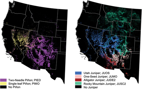
The quantification of PJ AGB on a broad scale is challenging due to its distinctive within-ecosystem heterogeneity and spatiotemporal variability (R. F. Miller et al. 2019; Romme et al. 2009). PJ woodland heterogeneity is, in part, due to the diversity of topography and climate across its range. They range spatially from forest-like conditions with high AGB, large trees, and high stand density to savanna-like conditions with low AGB, small trees, and low stand density (R. F. Miller et al. 2019; Romme et al. 2009). PJ woodlands have a complex history of afforestation and deforestation; they are sensitive to climate fluctuations, with historical wet periods leading to woodland infilling and range expansion (R. F. Miller et al. 2019), and drought periods leading to widespread mortality (Breshears et al. 2005; Shaw, Steed, and Deblander 2005). The proportional abundances and mixtures of piñon pine and juniper species differ regionally and are heavily influenced by the amount and seasonality of precipitation (Jacobs 2008; R. F. Miller et al. 2008; Romme et al. 2009). There are four dominant juniper species and two dominant piñon species in PJ woodlands: Utah juniper (Juniperus osteosperma; hereafter abbreviated as JUOS), one-seed juniper (Juniperus monosperma; JUMO), alligator juniper (Juniperus deppeana; JUDE2), Rocky Mountain juniper (Juniperus scopulorum; JUSC2), two-needle piñon (Pinus edulis; PIED), and single-leaf piñon (Pinus monophylla; PIMO) (Figure 1). Within the extent of PJ woodlands, PIMO and the majority of JUOS are predominantly found in the regions characterized by high winter and spring precipitation but lower summer precipitation. On the other hand, JUSC2 and PIED ranges extend across the North American summer monsoon boundary, meaning that they experience peaks of both summer and winter precipitation. In contrast, JUMO and JUDE2 are prevalent in regions influenced by the summer monsoon (Jacobs 2008; Romme et al. 2009).

PJ woodland heterogeneity is also due to natural and human disturbances that can lead to widespread mortality events. Disturbances such as drought (Breshears et al. 2005; Kannenberg et al. 2021; Shaw, Steed, and Deblander 2005), insect attacks (Anderegg et al. 2015; Gaylord et al. 2013), wildfires (Floyd, Hanna, and Romme 2004), and tree chaining (Ernst-Brock et al. 2019; Redmond et al. 2013) can contribute to PJ mortality. PJ mortality-inducing disturbances are further exacerbated by the impacts of climate change, such as the recent anomalously high temperatures in the western US (Williams, Cook, and Smerdon 2022). The extent and abundance of PJ woodlands makes them important to map, but the diversity of species compositions, disturbances, climate, and topography across space and time makes them especially challenging to quantify.

Direct quantification of PJ AGB can only be achieved through destructive tree harvesting, which is impractical on large scales (Huang et al. 2009). A more feasible approach involves linking field-collected stem measurements to allometric models to yield tree- or plot-level AGB estimates, which can in turn be linked to remotely sensed data, enabling broad-scale AGB estimation (Saarela et al. 2020). Remote sensing techniques offer a faster, less labor-intensive method for broad-scale AGB mapping (Eisfelder, Kuenzer, and Dech 2012). However, applying remote-sensing-based AGB estimation to PJ and dryland woodlands with similar structures presents its own challenges. PJ woodlands, characterized by relatively short trees, low canopy covers, extensive exposure of understory vegetation and soils, and small, nonuniform tree crown shapes, introduce complexities to remote sensing AGB mapping efforts (Campbell et al. 2020; Huang et al. 2009; Smith et al. 2019).

Airborne laser scanning (ALS) is a high-resolution, three-dimensional remote sensing method that has the ability to address the challenges associated with capturing the heterogeneous structure of PJ woodlands by offering more in-depth insights into vegetation structure than passive optical and active radar systems (Lefsky et al. 2002). Robust, quantitative measures of vegetation structure can be derived from ALS point clouds and utilized as AGB predictor variables in statistical and machine learning models, such as random forest (RF) algorithms (Ayrey et al. 2019; Campbell et al. 2021, 2023; Torre-Tojal et al. 2022). RFs are widely used in ecological modeling due to their ability to handle large datasets with numerous predictor variables, flexibility with continuous and discrete variables, and independence from assumptions in parametric modeling approaches (Breiman 2001; Cutler et al. 2007).

Despite the vital role of PJ woodlands in providing ecosystem services in the American Southwest, there are few targeted efforts to map PJ AGB using ALS (Campbell et al. 2021, 2023; Krofcheck et al. 2016; Sankey et al. 2013; Wu et al. 2016). Further, those that exist describe local-scale models which capture only a small fraction of PJ ecosystem diversity. Thus, there remains a high degree of uncertainty surrounding the extent to which results from these studies are transferable to other, ecologically distinct portions of the PJ woodland range. While several US-wide across-ecosystem AGB maps exist (e.g. Neeti and Kennedy 2016), their lack of tailoring to the unique ecosystem characteristics of PJ raises concerns about their potential to misrepresent total PJ AGB. To comprehensively map PJ AGB across its range, it is essential to first quantify the extent to which within-ecosystem heterogeneity influences model transferability.

Transferability, in the context of this study, refers to a model’s ability to make accurate predictions in novel conditions. Transferability, also referred to as generalizability, cross-applicability, or transference (Yates et al. 2018), is assessed and using model performance metrics (Sequeira et al. 2018; Yates et al. 2018). Our definition of transferability is comparable to other definitions of transferability in ecological research. Wenger and Olden (2012) “… define the transferability of a model as the accuracy of its predictions for an independent data set” and Yates et al. (2018) defines transferability as the “… capacity of a model to produce accurate and precise predictions for a new set of predictors that differ from those on which the model was trained.” Further, Sequeira et al. (2018) defines transferability as “… the ability of a model to predict biodiversity metrics in novel environments.” It is worth distinguishing transferability from transfer learning – a related but different concept. Transfer learning is a deep learning technique that uses data pre-trained on one task to improve performance on a related training task (Jiang et al., 2022), while transferability is the degree to which a model built on one dataset can be applied to novel data and is typically expressed in model performance metrics on the test data. Assessing model transferability is an important but often overlooked step in ecological modeling of diverse, wide-ranging ecosystems, particularly when seeking broadly applicable range-wide models (Randin et al. 2006). For example, there could be two PJ woodlands with equal AGB, one in a high-elevation, cooler, moister setting, and one in a low-elevation, warmer, drier setting. The favorable ecological conditions in the former site would tend to promote the growth of higher-biomass trees, whereas the less favorable conditions in the latter site would tend to restrict growth. Thus, for these sites to have the same AGB would likely mean that the former has fewer, larger trees, and the latter has more, smaller trees. ALS may struggle to recognize that the AGB in these two locations is the same, given their structural differences. This would represent a challenge to model transferability – the nature of which we specifically aim to explore in this study. Hence, this research seeks to further the development of a more accurate and regionally representative quantification of PJ AGB across its range. The objectives of this study were to:

1. Evaluate PJ woodland AGB model transferability by constructing ALS-driven RF regression models using two clustering categories: one based on environment and a second based on species composition.

2. Explore factors influencing model transferability by comparing model performance metrics and cluster characteristics.

3. Generate and assess the performance of a field-data-based source-stratified range-wide model of PJ AGB.

2. Methods

2.1. Study area and field data

We utilized field reference data collected within PJ woodlands across the states of Arizona, Colorado, Nevada, New Mexico, and Utah. In the field reference dataset, the recorded PJ tree species included JUOS, JUDE2, JUSC2, JUMO, PIED, and PIMO (Figure 1). We also recorded eight plots within the study area that had the PIMO species variety Arizona piñon pine (Pinus monophylla var. fallax; PIMOF). Due to its small quantity and for the purposes of this study, PIMOF was included within the broader category of the PIMO species.

In this study, we utilized two distinct sets of field data to comprehensively examine the AGB distribution of PJ woodlands. The first set involved dedicated field data collection with the explicit goal of mapping PJ AGB across its entire range. Between 2021 and 2022, the Piñon-Juniper BiOmass Over Space and Time (PJBOOST) dataset was collected (Table 1). PJBOOST consists of 18 separate sites, each containing approximately 10 plots, for a total of 177 30 m × 30 m square plots spread across PJ woodlands in Arizona, Colorado, Nevada, New Mexico, and Utah. We strategically designed the site collection to capture a diverse range of AGB, environmental conditions, and species compositions. Specifically situated in areas with recent, high-quality airborne lidar data, these sites were chosen on accessible public lands predominantly covered by PJ vegetation. Plots within these sites were placed opportunistically to ensure the capture of significant variations in within-site AGB.

For each plot in PJBOOST, we recorded the GPS coordinates for the four plot corners and the plot center. A Trimble R1 or R2 GPS receiver was employed for accurate positioning of our plots, with an average positional accuracy of 0.62 meters among all plot coordinates captured. Additionally, detailed information about each tree within a plot was documented, including tree species, and either the diameter at root collar (DRC) or the diameter at breast height (DBH), depending on tree species and according to the recommendations of the USDA Forest Inventory and Analysis (FIA) program. While PJBOOST intentionally covered a substantial portion of the PJ woodland’s total geographic extent, we opted to compile supplementary field data sourced from a variety of individual researchers, institutes, and agencies to gain a broader and more representative sampling of vegetation conditions (Table 1).

There were multiple requirements of both the ALS data and plot attributes for a plot to be included in the field reference dataset. Akin to the PJBOOST collection procedures, plot locations and dimensions, plot collection date, as well as the species, condition (live vs. dead), and the DRC or the DBH were required for every tree. In terms of the timing of ALS and field plot collection, there were three key requirements: (1) the field data overlaps existing, recent (2013 – present), high-quality (USGS QL1 or QL2), and freely available ALS data, (2) the plot was collected no earlier than 2013, and (3) and there were no significant disturbances between the time of field plot collection and ALS data collection. To determine if a disturbance occurred between the time of field plot collection and ALS data collection, we cross-referenced the data collection dates with the LANDFIRE Vegetation Disturbance data (LANDFIRE 2020). Further, plots needed to exhibit visual agreement between their recent high-resolution aerial imagery and their corresponding AGB values. For example, if a plot had very high canopy cover in imagery but a very low recorded AGB, the plot was removed from the dataset, as canopy cover and AGB tend to be highly correlated in PJ woodlands (Filippelli et al. 2020). In addition, plot AGB density could not exceed the maximum AGB density of 234.4 Mg/ha for PJ-dominated plots, as determined by an analysis of all PJ plots present within the USDA FIA database. Lastly, plots must have an area larger than 200 m² as areas smaller than that may produce unstable AGB estimates, given the spatial heterogeneity and sparseness of PJ woodland structure. In total, the field reference dataset we used for modeling comprised 16,032 live PJ trees within 497 plots from eight sources (Table 1) (Campbell and Eastburn 2024).

Table 1. Summary of field data sources.

Field Dataset Source	Dataset Abbreviation	Number of Plots	Square (S) or Circle (C) Plot Geometry	Square Plot Dimensions, Circle Plot Radius, or Range of Circle Plot Radii (m)	Start Year	End Year
PJBOOST, Campbell and Eastburn	PJBOOST	177	S	30 x 30	2021	2022
Southwestern Lidar Monitoring Network (Blackburn, Buscaglia, and Sánchez Meador 2021; Tenneson et al. 2018)	SLMN	152	C	8.0–16.1	2013	2015
Coupled Natural and Human Systems Program, San Juan County, Kerr and Kannenberg	SJC	70	C	15.0–18.0	2018	2020
Tusayan Fuels Treatment Study, Ecological Restoration Institute (Huffman et al. 2009, 2019)	ERI	40	C	11.3	2017	2017
Carbon Monitoring System Program, Cedar City	CEDAR	19	C	11.4	2020	2020
University of Nevada Reno, (Flake and Weisberg 2019; Greenwood and Weisberg 2008)	UNR	16	C	17.9	2014	2015
San Juan National Forest Transect, Anderegg	AND	15	C	18.0–25.0	2019	2019
Colorado Forest Restoration Institute	CFRI	8	C	11.3	2014	2014

2.2. Allometry from field data

PJ and other dry woodlands have been understudied compared to other tree-dominated systems – particularly those traditionally characterized as being “forest.” This may be attributed to their perceived lower ecological value (i.e. lower biomass), economic value (i.e. lower timber value), and aesthetic value. Whatever the cause, the comparably sparse research on PJ woodlands, in combination with their structural complexity has contributed to a similar sparseness of and inconsistency between PJ allometric models. The existing equations that relied solely on DRC and did not consider other AGB-associated variables like tree height and canopy width were even more limited. While some allometric equations for woodland trees incorporated other tree biometrics, they only existed for some and of the tree species found within our field data (e.g. Grier, Elliott, and McCullough 1992; E. L. Miller, Meeuwig, and Budy 1981). We decided to use generalized allometric equations of Chojnacky et al. (2014) because they could be broadly applied to the PJ species we encountered, rather than compiling disparate, species-specific models from several different studies.

The strength of the Chojnacky et al. (2014) generalized biomass equations lies in their meta-analytical approach, which takes many individual species-level models into account. This approach enhances the applicability of their models, as it considers a broader range of species and conditions. The updated generalized equations by Chojnacky et al. (2014) were chosen over their predecessor, the Jenkins et al. (2003) equations, due to the increased taxonomic division for woodland species. The Chojnacky et al. (2014) generalized biomass equation for woodland Pinaceae (piñons) incorporated allometric data from five studies, with a coefficient of determination (R²) of 0.86, while the woodland Cupressaceae (junipers) generalized biomass equation included data from six studies, with an R² of 0.91. Therefore, we chose the Chojnacky et al. (2014) equations for our allometries for both their meta-analytical approach and the resulting accuracies achieved in their generalized models.

For each plot in the field dataset, we calculated AGB at the individual tree level then aggregated it to the plot level using a multi-step process. First, we used Eq. 1(1) $\begin{array}{c}ln\left(\mathit{AGB}\right)={\beta }_0+{\beta }_1\mathit{d}\end{array}$(1) (Chojnacky, Heath, and Jenkins 2014) to calculate AGB per tree in kg:

(1) $\begin{array}{c}ln\left(\mathit{AGB}\right)={\beta }_0+{\beta }_1\mathit{d}\end{array}$(1)

where $\mathit{AGB}$ is aboveground biomass in kg, ${\beta }_0$ and$\mathit{\hspace{0.17em}}{\beta }_1$ are taxonomic family-specific coefficients (Chojnacky, Heath, and Jenkins 2014), and $\mathit{d}$ is DRC or DBH in cm. Eq. 1(1) $\begin{array}{c}ln\left(\mathit{AGB}\right)={\beta }_0+{\beta }_1\mathit{d}\end{array}$(1) utilized both DRC and DBH as diameter inputs, depending on the tree group and taxa to which the recorded tree species belonged. Table 5 in Chojnacky et al. (2014) specified that woodland tree groups use DRC, while hardwood and conifer groups use DBH as the diameter input. This approach eliminated the need for converting between DRC and DBH. In the case of multi-stemmed trees, we used Eq. 2(2) $\mathit{d}=\sqrt{\sum _{\mathit{i}=1}^n{d}_i^2}$(2) (Chojnacky and Rogers 1999) to derive a single-diameter-equivalent measurement for a multi-stem tree:

(2) $\mathit{d}=\sqrt{\sum _{\mathit{i}=1}^n{d}_i^2}$(2)

where$\mathit{\hspace{0.17em}}\mathit{n}$ is the number of stems measured and $d_i$ is the diameter of a single stem i for each stem within a multi-stemmed tree. We then used the resulting single diameter measurement from Eq. 2(2) $\mathit{d}=\sqrt{\sum _{\mathit{i}=1}^n{d}_i^2}$(2) as the diameter in cm in Eq. 1(1) $\begin{array}{c}ln\left(\mathit{AGB}\right)={\beta }_0+{\beta }_1\mathit{d}\end{array}$(1) to estimate AGB for a single tree. Lastly, we calculated estimates of AGB density per plot in megagrams per hectare (Mg/ha) by computing the sum of the AGB estimates calculated in Eq. 1(1) $\begin{array}{c}ln\left(\mathit{AGB}\right)={\beta }_0+{\beta }_1\mathit{d}\end{array}$(1) and dividing this value by the area of the plot.

2.3. ALS-Derived predictor variables

We acquired ALS data from 24 datasets, collected by the USGS 3D Elevation Program (Sugarbaker et al. 2014) and the National Center for Airborne Laser Mapping (NCALM) (Table 2). In cases where multiple ALS datasets overlapped field plots, we used the most recent ALS dataset. All ALS data underwent the following pre-processing steps, using a combination of LAStools (v230330) (Isenburg 2006) and the R lidR library (v4.0.3) (Roussel and Auty 2023; Roussel et al. 2020) prior to modeling for consistency and quality assurance:

1. Reprojection into the local UTM coordinate system.

2. Noise removal, using the lasnoise function in LAStools.

3. Height normalization, to compute above ground lidar point height relative to an interpolated ground surface.

4. Clipping to the geometry of each field plot that overlapped the ALS data’s extent.

Table 2. Summary of ALS projects. Shown is the project name from either USGS 3D Elevation Program or NCALM, the average pulse density in pulses/m² of each ALS project catalog, the number of field plots acquired from each project, and the project collection start and end dates.

ALS Project Name	Pulse Density (pulses/m^2)	# of Plots	Start Date	End Date
AZ_Coconino_2019_B19	9.9	18	2019/08/16	2019/08/20
AZ_USFS_3DEP_Processing_2019_D20	16.7	63	2013/08/24	2014/10/12
CA_AZ_FEMA_R9_Lidar_2017_D18	6.9	87	2018/01/06	2019/02/24
CO_SanLuisJuanMiguel_2020_D20	6.1	24	2019/09/21	2020/10/04
CO_Southwest_NRCS_2018_D18	6.0	9	2018/10/05	2019/09/24
NM_NorthWest_2018_D19	4.2	10	2018/11/14	2018/11/28
NM_SouthCentral_2018_D19	4.4	27	2018/11/20	2019/06/06
NV_NorthWestElko_2020_D20	4.2	18	2020/10/09	2020/11/08
NV_WestCentral_EarthMRI_2020_D20	4.6	16	2020/10/15	2020/11/04
USGS_LPC_AZ_VerdeKaibab_B1_2018_LAS_2019	12.5	51	2018/08/10	2018/09/07
USGS_LPC_AZ_VerdeKaibab_B2_2018_LAS_2019	5.2	11	2018/08/10	2018/09/08
USGS_LPC_NM_North_Central_B2_2016	6.2	8	2016/11/29	2018/10/31
USGS_LPC_NM_RioSanJose_2016_LAS_2019	3.3	10	2016/12/15	2017/06/11
USGS_LPC_UT_BoxElder_2018_LAS_2019	13.8	7	2018/09/04	2019/03/19
USGS_LPC_UT_Central_QL1_B2_2018_LAS_2019	19.8	16	2018/06/05	2018/09/03
USGS_LPC_UT_MonroeMoutain_2016_LAS_2018	12.8	2	2016/08/27	2016/09/11
USGS_LPC_UT_Southern_B1_2018_LAS_2019	4.4	11	2018/04/27	2018/10/12
USGS_LPC_UT_Southern_B2_2018_LAS_2019	4.0	1	2018/04/27	2018/10/12
USGS_LPC_UT_Southern_QL1_2018_LAS_2019	24	12	2018/04/27	2018/07/29
UT18_Dennison	15.3	67	2018/06/02	2018/06/03
UT_StateWide_2018_A18	22.8	6	2018/09/08	2018/09/09
UT_StatewideCenSouth_2020_A20	4.0	3	2020/09/20	2021/06/26
UT_StatewideKane_2020_A20	4.2	10	2019/10/11	2019/11/16
UT_StatewideSouth_2020_A20	14.9	10	2020/05/02	2020/08/23

To form the basis of AGB predictions in PJ woodlands, we generated a suite of 70 metrics, derived from ALS point clouds, as outlined in Table 3 (Campbell et al. 2021). These metrics, categorized as area-based and tree-based, characterize the vegetation within field plots. The area-based metrics summarize point cloud characteristics across the entire plot. In contrast, tree-based metrics summarize point cloud features within individual tree crowns, delineated from a canopy height model that is derived from the height-normalized point cloud of each plot. Treetop detection was conducted using the lmfauto() function and tree segmentation was conducted using the silva2016() function in the R package lidR (v4.0.3) (Roussel and Auty 2023; Roussel et al. 2020).

Table 3. Area and tree-based metrics derived from field plot coincident ALS point clouds. Adapted from (Campbell et al. 2021).

Abbreviation	Area (A) or Tree (T) Based Metric	Metric
cc	A	Canopy cover: the number of first returns at or above breast height (1.37 m) divided by the total number of first returns
cd	A	Canopy density: the number of all returns at or above breast height (1.37 m) divided by the total number of all returns
p.x	A	xth height percentile of rank-ordered point heights from 5th to 100th at a 5-percentile interval
mh	A	Mean of all point heights
mg.ag	A	Mean of aboveground point heights
sd	A	Standard deviation of all point heights
sd.ag	A	Standard deviation of aboveground point heights
skew	A	Skewness of all point heights
skew.ag	A	Skewness of aboveground point heights
kurt	A	Kurtosis of all point heights
kurt.ag	A	Kurtosis of aboveground point heights
vrd.x.y	A	Vertical relative point densities between heights x and y: the number of points between x and y divided by the total number of points between 0 and 5 m in height (all points in a given area), for all height ranges between 0 and 5 m at an interval of 0.5 m [[x =0, y =0.5], [x =0.5, y =1], […], [x =4.5, y =5]]
vnrd.xy	A	Vertical normalized relative point densities between heights x and y: the number of the number of points between x and y divided by the number of points between 0 and y (only points within height range and below), for all height ranges between 0 and 5 m at an interval of 0.5 m [[x =0, y =0.5], [x =0.5, y =1], […], [x =4.5, y =5]]
cr.num	T	Number of automatically delineated tree crowns within a plot
cr.mh	T	Mean crown height of automatically delineated tree crowns within a plot
cr.ma	T	Mean crown height aboveground of automatically delineated tree crowns within a plot
cr.qh.xx	T	xx’th quantile of crown heights of automatically delineated tree crowns within a plot
cr.qa.xx	T	xx’th quantile of crown heights aboveground of automatically delineated tree crowns within a plot

2.4. Plot clustering

To understand how within-ecosystem diversity influences model transferability, we identified two key categories driving diversity in the PJ woodland ecosystem: environment and species composition. Transferability involves training models on one dataset and then testing them on another distinct dataset to assess its performance in new conditions. To apply this concept with our data, we nonrandomly divided our full field dataset into distinct clusters for each category. A distinct cluster, in the context of this study, represents data that are internally homogeneous but sufficiently different from other clusters, simulating the novel conditions required to assess transferability (Wenger and Olden 2012; Yates et al. 2018). The distinct clusters for each category are hereafter referred to as “environmental clusters” and “species composition clusters.” A nonrandom train/test split splits data into training and testing based on some predetermined criteria, while a random train/test split randomly splits data into training and testing sets, regardless of underlying patterns in the data. Because a random approach cannot guarantee distinct train and test sets, which are necessary for a transferability assessment, it is not a suitable method for dividing data for our transferability models (Wenger and Olden 2012). However, a random training and testing approach would provide an estimate of broader relationships within the data and would thus be more suited to a range-wide modeling approach. Our categorical identification of drivers of ecosystem diversity and subsequent nonrandom clustering approach allows us to use the distinct clusters within each category as proxies for novel conditions, facilitating the direct evaluation of model transferability between each distinct cluster within each category. We note, however, that we not explicitly testing how membership to distinct environmental and species clusters drive variability in AGB; we are testing the degree to which the same ALS metrics can predict the same AGB in distinct clusters.

To form the basis of clustering for the environmental clusters, we utilized PRISM’s 30-year normal datasets from 1991 to 2020 to derive temperature, precipitation, vapor pressure deficit VPD, and elevation for each plot (PRISM Climate Group at Oregon State University 2022). Specifically, we calculated the minimum, maximum, and mean daily temperatures. Additionally, we derived summer and winter minimum and maximum temperatures by averaging mean temperature over the summer months (July – September) and winter months (December – February). Furthermore, we calculated the mean precipitation, the minimum and maximum VPD, and plot elevation. We also derived the summer and winter precipitation for each plot. The second clustering category, hereafter referred to as the species composition category, clustered plots based on their proportional PJ species composition.

We employed the k-means clustering algorithm for both the environmental and species composition categories, choosing it for its simplicity, interpretability, and scalability. The optimal number of clusters was determined through exploration of various k values, considering factors like result interpretability (fewer clusters facilitate a better understanding of factors affecting transferability), cluster homogeneity (differences within clusters should be relatively small in comparison to differences between clusters), and cluster size robustness (too many clusters will yield groupings of plots too few to train or test predictive models) (Jain 2010). To ensure effective separation of clusters, we evaluated the proportion of variance explained (η²) for each k value. The η² was calculated for each k value by dividing the sum of squares between clusters by the total sum of squares. We aimed for a balance between a high η² and sufficient cluster sizes to determine the number of clusters for each category.

2.5. Transferability models

First, we implemented a variable selection procedure using the R package Variable Selection Using Random Forests (VSURF) (v1.2.0) (Core Team 2021; Genuer, Poggi, and Tuleau-Malot 2015). VSURF leverages the capabilities of RF to effectively rank and select the most important predictor variables for model building. Although many other algorithms exist for variable selection (e.g. recursive feature elimination, genetic algorithms, etc.), we chose VSURF for two main reasons. First, it relies solely on RF, which ensures that the variable selection procedure is optimized for the very same machine learning algorithm we used for final modeling. Second, it has been shown to be effective in wide-ranging modeling studies, including several focused on remote sensing-based biomass estimation (e.g. Campbell et al. 2021; Chen et al. 2022; Grüner, Astor, and Wachendorf 2021).

While variable selection procedures like VSURF can potentially remove useful predictors, and thus lead to misinterpretations of variables being deemed “unimportant,” our goal in using VSURF was primarily for improving predictive accuracy. VSURF’s three-step selection procedure iteratively reduces model complexity and variable redundancy in its three-step variable selection procedure. It first removes predictor variables of low importance from consideration, then selects all variables important to the response variable for interpretation purposes, and finally eliminates redundant variables to create a parsimonious set of variables for prediction purposes (Genuer, Poggi, and Tuleau-Malot 2015). Given that the primary objective of this study was to assess model performance, we used the selected variables from the last of the three VSURF steps. Had we been more focused on understanding predictor–response relationships, we might have selected the variables from the second of the three steps.

We then generated RF regression models for each cluster in the two categories using the R ranger package (v0.15.1) (Wright and Ziegler 2017). In ecological research, RF has been shown to be an optimal (Cao et al. 2018), or suitable (Fekety et al. 2018; Gleason and Im 2012; Torre-Tojal et al., 2022), algorithm to predict forest attributes using lidar-derived data. We chose RF models over other machine learning algorithms due to their ability to handle large datasets, numerous predictor variables, complex relationships between variables, and their low sensitivity to hyperparameter tuning, without the pitfall of overfitting. To obtain optimal RF hyperparameters, we tuned each RF model using the R tuneRanger package (v0.5) (Probst, Wright, and Boulesteix 2018). tuneRanger uses a model-based optimization tuning strategy to automatically determine the optimal minimum node size (the fewest number of training samples contained within a tree’s terminal node), sample fraction (the proportion of data used to train the model on each iteration in the bagging process), and mtry (the number of predictor variables tested at each decision tree split) for an RF model (Probst, Wright, and Boulesteix 2018; Wright and Ziegler 2017).

The RF model for a distinct cluster is then tested on one other distinct cluster at a time, with all other clusters withheld from testing. This cross-validation process was repeated for all clusters until the data from each distinct cluster was used to train an RF model, and that model was tested on one other distinct cluster at a time while completely withholding the remaining clusters. We calculated the R² (Eq. 3(3) $R^2=1-\frac{\sum {\left(y_i-{\hat{y}}_{\mathit{i}}\right)}^2}{\sum {\left(y_i-\bar{y}\right)}^2}$(3) ) and relative root mean square error (rRMSE) (Eq. 4(4) $\mathit{rRMSE}=\frac{\sqrt{\frac{\sum {\left(y_i-{\hat{y}}_{\mathit{i}}\right)}^2}{\mathit{n}}}}{\bar{y}}$(4) ) for each cluster to serve as our quantitative measures of transferability.

(3) $R^2=1-\frac{\sum {\left(y_i-{\hat{y}}_{\mathit{i}}\right)}^2}{\sum {\left(y_i-\bar{y}\right)}^2}$(3)

(4) $\mathit{rRMSE}=\frac{\sqrt{\frac{\sum {\left(y_i-{\hat{y}}_{\mathit{i}}\right)}^2}{\mathit{n}}}}{\bar{y}}$(4)

where $y_i$ is the measured value, ${\hat{y}}_{\mathit{i}}$ is the predicted value, $\bar{y}$ is the mean of measured values, and $\mathit{n}$ is the number of observations. To internally assess model performance, we performed a 10-fold cross validation on each cluster. We furthered our investigation of environmental and species composition transferability by comparing model R² and rRMSE results to a thorough examination of cluster characteristics. Our goal was to glean insights into the distinct characteristics of each cluster to discern ecologically driven explanations for transferability model performance. In the environmental category, we examined the distribution of climate and topography variables across clusters. For the species composition category, we examined the proportions of each PJ species within each cluster.

2.7. Range-wide modeling

As our final step in the PJ AGB modeling process, we built a series of bootstrapped, comprehensive, range-wide predictive models of PJ AGB. We used bootstrapping to yield a more broadly representative range of performance metrics rather than a potentially biased set that may result from a singular training/test split (Wager, Hastie, and Efron 2014). To ensure the representation of field data from the range of PJ woodlands and data sources in both training and testing samples, we employed a stratified sampling technique based on the eight field data sources. For each of the 10,000 bootstrap iterations, we randomly selected approximately 70% of the plots from each field data source. The remaining 30% from each source was set aside and used to test the model. For each model, we used the variables selected by the initial VSURF as predictors of AGB. The range-wide model underwent a single tuning process using the tuneRanger package (v0.5) (Probst, Wright, and Boulesteix 2018). Next, we calculated variable importance for the VSURF variables, measured as the increase in mean squared error resulting from the random permutation of predictor variables. Further, we calculated model R² and rRMSE, and the median distributions of each to get measures of central tendency. Lastly, we calculated the 25^th (Q₂₅) and 75^th (Q₇₅) quartiles and the interquartile range (IQR) (IQR = Q₇₅ - Q₂₅) from the bootstrap analysis results to characterize the spread in R² and rRMSE distributions.

3. Results

3.1. Allometry and variable selection

Allometrically derived AGB among the 497 field plots resulted in PJ AGB distribution spanning from 0.003 Mg/ha to 224.7 Mg/ha, with a median AGB of 43.7 Mg/ha (Figure 2). The VSURF reduced the number of potential predictor variables for the RF models from 70 to six (Figure 3), representing approximately 9% of the original suite of predictor variables (Table 3). In order of variable importance, our predictor variables were canopy cover, mean height aboveground, canopy density, mean height, skewness, and vertical relative normalized point density between 0.5 m and 1 m. See Table 3 for further metric descriptions.

Figure 2. Distribution of PJ woodland AGB across 497 field plots, in Mg/ha. The median of plot AGB is 43.7 Mg/ha and is represented by the dashed line. The first quartile (Q₂₅) is 25.1 Mg/ha, and the third quartile (Q₇₅) is 72.9 Mg/ha. Both are represented by solid lines.

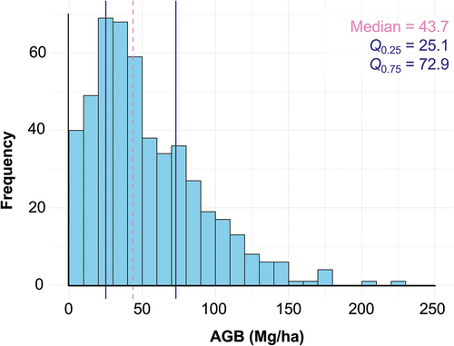
Figure 3. Increase in mean squared error in Mg²/ha² of VSURF-chosen ALS predictor variables. Abbreviations, listed in order of variable importance, stand for canopy cover (cc), mean height aboveground (mh.Ag), canopy density (cd), mean height (mh), skewness (skew), and vertical normalized relative point density between 50cm and 100cm (vnrd.50.100). See Table 3 for further metric descriptions.

3.2. Environmental category clustering

We experimented with k values to find the appropriate number of k-means clusters for the environmental category. Our chosen number of clusters was based on the k value that exhibited both sufficiently large cluster sizes and a high η². Three clusters were deemed insufficient with an η² of 60.9%. Four clusters yielded improvement to 68.6% and five clusters improved the η² marginally to 71.1% (Table 4). Since both four and five k-means clusters were sufficiently large, we decided to divide the environmental category into four clusters (Figure 4) because there was only marginal improvement of the η² from four to five clusters. The four clusters are of sizes 126, 102, 125, and 144 (Table 4).

Table 4. Results of environmental category k-means clustering using different k values.

k Value	Cluster Sizes	η^2
2	141, 356	44.6%
3	225, 143, 129	60.9%
4	126, 102, 125, 144	68.6%
5	126, 43, 140, 121, 67	71.1%

We analyzed the distribution of environmental clustering variables (Figure 5) and characterized the clusters in terms of their temperature, precipitation, VPD, and elevation as follows.

Figure 4. Environmental category clusters and the distribution of their plots across the PJ woodland range. Points represent plot locations and are underlaid by the LANDFIRE EVT defined extent of PJ woodlands (LANDFIRE 2020).

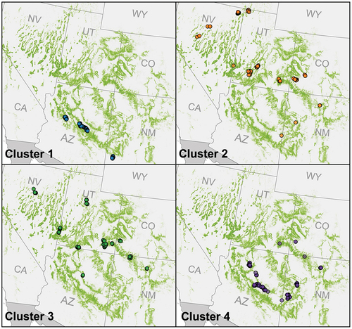
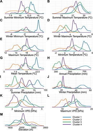
• Cluster 1: high temperature, high precipitation, high VPD, and low elevation.

• Cluster 2: low temperature, moderate precipitation, low VPD, and high elevation.

• Cluster 3: moderate-high temperature, low precipitation, moderate-high VPD, and low-moderate elevation.

• Cluster 4: moderate temperature, moderate precipitation, moderate VPD, and moderate elevation.

Notably high amounts of precipitation and high temperatures distinguished cluster 1 from the other clusters (Figure 5). Additionally, cluster 1 was spatially unique (Figure 4); cluster 1 plots were mainly concentrated in Arizona, with a few plots in southwestern New Mexico, while the other clusters were distributed across four or more states (Figure 4).

Figure 5. Density plots of the temperature, precipitation, VPD, and elevation for each environmental cluster. Values are obtained for each plot based on the geographical plot center. a) Summer minimum temperature. b) Summer maximum temperature. c) Winter minimum temperature. d) Winter maximum temperature. e) Maximum daily temperature. f) Minimum daily temperature. g) Mean annual daily temperature. h) Daily precipitation. i) Summer precipitation. j) Winter precipitation. k) Minimum VPD. l) Maximum VPD. m) Elevation.

3.3. Species composition category clustering

Similar to the environmental category, we experimented with k values and chose the number of k-means clusters for the species composition clustering based on a high η², and sufficiently large cluster sizes. Four clusters yielded significant improvement to an η² of 80.3% from a three cluster η² of 70.5%. Five clusters yielded only a marginal improvement of η² to 81.4% (Table 5). Since cluster sizes for five k values were not all sufficiently large with one cluster consisting of 25 plots, and there was only small improvement of η² between four and five k values, we chose four as our number of species composition clusters (Figure 6). The four clusters are of sizes 152, 142, 145, and 58 (Table 5).

Figure 6. Species composition category clusters and the distribution of their plots across the PJ woodland range. Points represent plot locations and are underlaid by the LANDFIRE EVT defined extent of PJ woodlands (LANDFIRE 2020).

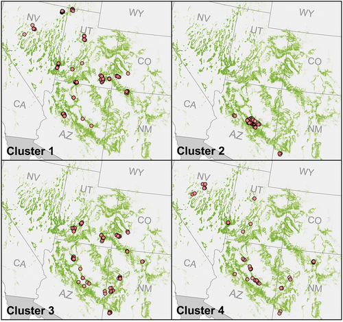
Table 5. Results of species composition category k-means clustering using different k values.

k Value	Cluster Sizes	η^2
2	275, 222	27.9%
3	180, 143, 174	70.5%
4	152, 142, 145, 58	80.3%
5	142, 137, 78, 25, 115	81.4%

As determined by the proportion of PJ species AGB in a plot (Figure 7), we characterized the four species composition clusters as follows.

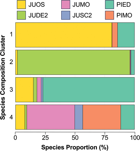
• Cluster 1: JUOS dominated with PIED and some PIMO.

• Cluster 2: JUDE2 dominated with some PIED.

• Cluster 3: PIED dominated with JUOS and some JUMO and JUDE2.

• Cluster 4: JUMO and PIMO dominated with JUOS, JUSC2, and PIED.

Cluster 2, characterized by the dominance of JUDE2 with some PIED (Figure 7), represents a relatively distinct species composition. The JUDE2 species dominance that occurs in Cluster 2 is distinct in that JUDE2 is not found in abundance in any other cluster. Like environmental cluster 1 (Figure 4), cluster 2 is also geographically unique in comparison to other clusters (Figure 6). While other clusters are dominated (>75%) by one PJ species, cluster 4 is has high proportional abundances of both JUMO (40%) and PIMO (32%) (Figure 7).

Figure 7. Proportion of PJ woodland species in each species composition cluster.

3.4. Transferability analysis

When using the environmental clusters as the basis of transferability modeling, we observed similar mean training model performance across clusters. Mean training R² ranged from 0.49 to 0.52 and mean rRMSE ranged from 0.51 to 0.55 (Figure 8). However, the mean testing R² and rRMSE had much wider ranges of model performance: the mean testing R² ranged from 0.43 to 0.65 and mean rRMSE ranged from 0.46 to 0.64 (Figure 8).

Figure 8. Transferability model performance for environmental clusters, containing three subfigures: (a) predicted (y-axis) versus observed (x-axis) AGB for models built using each training cluster (rows) applied to the prediction of each testing cluster (columns), with the solid red line representing a linear regression between predictions and observations, and the dashed black line representing the 1:1 relationship; (b) R² values for each of the transferability models depicted in A, with cells colored according to relative performance; and (c) rRMSE values for each of the transferability models depicted in A, with cells colored according to relative performance. In B and C, the models trained and tested on the same clusters are colored gray, as they do not measure transferability, but are provided for comparison to within-cluster model performance.

As shown in Figure 8, cluster 1 had higher training transferability (mean R² = 0.52; mean rRMSE = 0.55) than testing transferability (mean R² = 0.51; mean rRMSE = 0.64), based on the relatively high mean testing rRMSE. Testing R² and rRMSE values in cluster 2 were consistent between performance metrics and were indicative of high testing transferability. Cluster 2 had a mean testing R² of 0.65 and a complimentary low rRMSE of 0.48. Cluster 3 had comparable training (mean R² = 0.49; mean rRMSE = 0.54) and testing (mean R² = 0.43; mean rRMSE = 0.55) transferability. Like cluster 3, cluster 4 also had comparable training (mean R² = 0.51; mean rRMSE = 0.51) and testing (mean R² = 0.45; mean rRMSE = 0.46) transferability across performance metrics (Figure 8).

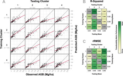
When using the species composition clusters as the basis of transferability modeling, we observed a small range of mean training model performance across clusters. Mean training R² ranged from 0.52 to 0.58 and mean rRMSE ranged from 0.47 to 0.51 (Figure 9). Meanwhile, the mean testing R² and rRMSE had much wider ranges of model performance: the mean testing R² ranged from 0.43 to 0.76 and mean rRMSE ranged from 0.37 to 0.62 (Figure 9).

Figure 9. Transferability model performance for species composition clusters, containing three subfigures: (a) predicted (y-axis) versus observed (x-axis) AGB for models built using each training cluster (rows) applied to the prediction of each testing cluster (columns), with the solid red line representing a linear regression between predictions and observations, and the dashed black line representing the 1:1 relationship; (b) R² values for each of the transferability models depicted in A, with cells colored according to relative performance; and (c) rRMSE values for each of the transferability models depicted in A, with cells colored according to relative performance. In B and C, the models trained and tested on the same clusters are colored gray, as they do not measure transferability, but are provided for comparison to within-cluster model performance.

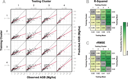
As shown in Figure 9, models tested on species composition cluster 4 exhibit strong model performance (mean R² = 0.76; mean rRMSE = 0.37). However, the inverse is observed, with relatively low transferability of cluster 4 to other clusters (mean R² = 0.52; mean rRMSE = 0.49). Cluster 3 models exhibit both a notable degree of applicability to other clusters (mean R² = 0.58; mean rRMSE = 0.47) and strong performance when subjected to testing from other cluster models (mean R² = 0.58; mean rRMSE = 0.41). Meanwhile, cluster 2 demonstrates high training transferability (mean R² = 0.57; mean rRMSE = 0.48) and low testing transferability (mean R² = 0.44; mean rRMSE = 0.62) across performance metrics. Lastly, cluster 1 has slightly higher training transferability (mean R² = 0.53; mean rRMSE = 0.51) than testing transferability (mean R² = 0.43; mean rRMSE = 0.55) (Figure 9).

3.5. Range-wide modeling

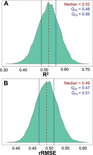
The range-wide model tuning resulted in the following hyperparameters: minimum node size = 7, sample fraction = 0.2977001, and mtry = 5. The bootstrapped accuracy assessment yielded a median R² distribution of 0.52 (Figure 10A) and a median rRMSE distribution of 0.49 (Figure 10B). Notably, both the R² and rRMSE distributions exhibit a low IQR (R² IQR = 0.08; rRMSE IQR = 0.04), suggesting limited variability and high precision across the 10,000 bootstrap iterations.

Figure 10. R² and rRMSE distribution of 10,000 bootstrapping iterations for the range-wide model. a) R² distribution. Dashed line represents median R² of 0.52 and solid lines represent the 25^th and 75^th quartiles of 0.48 and 0.56, respectively. b) rRMSE distribution. Dashed line represents median rRMSE of 0.49 and solid lines represent the represent the 25^th and 75^th quartiles of 0.47 and 0.51, respectively.

4. Discussion

This research represents a substantial effort to quantify ALS-driven PJ woodland AGB model transferability throughout the vast, complex dryland ecosystem. We utilized 24 ALS datasets and coincident field reference data from eight sources, which encompassed 497 plots and 16,032 PJ trees. Despite the challenges of mapping AGB across its complex ecosystem, including variability in measurement methods between data sources and uncertainty from allometric equations, our findings provide valuable insights toward mapping PJ AGB range-wide in a tailored and comprehensive manner. They provide us with an understanding of how range-wide models will perform when trained and applied across various portions of PJ’s wide and diverse range.

We decided to use both R² and rRMSE error metrics to provide a more comprehensive evaluation of model performance. R² gives an indication of how well predictions and observations correlate with other another, while rRMSE directly measures the accuracy of model predictions. By considering both metrics when evaluating a model, we can assess different aspects of the model’s performance. High R² values suggest that prevailing trends in higher or lower AGB can be predicted, even if the predictions and observations do not agree in magnitude. Conversely, low rRMSE values suggest agreement between predictions and observations, but do not necessarily indicate that high predictions correspond to high observations and low predictions correspond to low observations. For example, a model that predicts a random set of values close to the mean of observations may yield a low rRMSE, but also a very low R². Thus, while rRMSE may be a more direct measure of accuracy, R² complements rRMSE by providing additional information on the overall performance, explanatory power, and transferability of the model.

Our research was driven by the fundamental question: how does environmental and species composition variability within the PJ woodland ecosystem influence transferability and our ultimate ability to rigorously map AGB? The distinctiveness of both environmental cluster 1 and species composition cluster 2 within their respective categories offers the opportunity to delve into the influence of distinct environments on model transferability. We identified environmental cluster 1 as distinct due to its notably high temperatures and high precipitation amounts. We consider species composition cluster 2 to be distinct due to the dominance of JUDE2, which is either nonexistent or present in very small quantities in other clusters. Environmental cluster 1 and species composition cluster 2 were very similar; in fact, 84% of the plots in environmental cluster 1 were in species composition cluster 2, and 75% of the plots in species composition cluster 2 were in environmental cluster 1. When models were tested on these clusters, transferability was relatively low for both the environmental (mean testing R² = 0.51; mean testing rRMSE = 0.64) and species composition (mean testing R² = 0.44; mean testing rRMSE = 0.62) clusters. This points to the idea that distinct environments or species compositions could be misrepresented in current US-wide across-ecosystem AGB maps. This misrepresentation arises because across-ecosystem AGB maps often group distinct PJ woodlands together as one homogeneous forest type (Neeti and Kennedy 2016), when they are heterogenous in nature.

However, ecology alone may not be responsible for promoting or limiting transferability; we must also consider the statistical properties of the models. For example, those same distinct clusters (environmental cluster 1 and species composition cluster 2) featured relatively high training transferability in the environmental (mean training R² = 0.52; mean training rRMSE = 0.55) and species composition (mean training R² = 0.57; mean training rRMSE = 0.48) transferability analyses. We attribute this not to the ecological conditions in these clusters, but the fact that these clusters contain a wider representation of AGB values among their field plots. RF, by design, cannot extrapolate when making predictions. Thus, training a model with a wider range in the response variable promotes the ability to make a wider range of predictions. In effect, this will act to increase training R² and reduce training rRMSE, as seen in environmental cluster 1 and species composition cluster 2.

Species composition cluster 4 can provide insight into the impact of species diversity and proportional abundance on model transferability. Clusters 1, 2, and 3 are all composed of one PJ species in greater than 75% proportional abundance, while the remaining 25% is a combination of two to four other PJ species. Cluster 4 is distinct because it is dominated by two species: JUMO (40%) and PIMO (32%). The cluster 4 model exhibits excellent internal performance, with a high R² (0.80) and low rRMSE (0.31). We also observe that cluster 4 has, by far, the highest testing mean R² of 0.76 and the lowest mean testing rRMSE of 0.37. However, the mean training R² (0.52) and mean training rRMSE (0.49) indicate average cluster transferability. Therefore, we can conclude that models of PJ AGB trained on predominantly one species have high transferability to clusters that are diverse in both their number of species and relative abundance.

The range of AGB density in our training clusters notably impacted model performance. Plot AGB densities ranged from 0.003 to 224.7 Mg/ha, however 88.3% of the field plots had AGB density values below 100 Mg/ha, while the remaining 11.7% fell within the range of 100–224.7 Mg/ha. As a result, distributing the 11.7% of plots with very high AGB density across four clusters led to a scarcity of model training data for very high AGB density plots within each cluster. In fact, the maximum AGB density of species composition cluster 4 was 117.1 Mg/ha, with only four plots greater than 100 Mg/ha. Due to RFs inability to extrapolate beyond the range of training data they are provided, AGB density predictions for species composition cluster 4 were capped at their low AGB density maximum, irrespective of testing cluster.

Our range-wide model performed reasonably well regarding both the models R² and rRMSE distributions. The bootstrapped IQR of the rRMSE was relatively small (0.04), which suggests more reliable, consistent estimates of AGB prediction error from the model. However, the range wide model tended to over-predict lower AGB plots and under-predict higher AGB plots. The under-prediction of smaller values and over-prediction of larger values is a known behavior of RF regression models (Zhang and Lu 2012); however, it is partially mitigated through hyperparameter tuning and the collection of more diverse and representative training data. RF exhibits robustness against hyperparameter tuning in our transferability and range-wide models. Hyperparameter tuning results (see Appendix) revealed consistent trends in hyperparameter values across models. The generalized additive model line was mostly flat for all models, suggesting that hyperparameter tuning had minimal impact on model performance. The range of mtry values selected by tuneRanger was narrow, typically ranging between one and six while sample fraction varied widely, ranging from 0.2 to 0.68. Among the tuned hyperparameters, minimum node size showed the most consistent relationship with predictive error, with smaller values leading to lower predictive error.

We selected the RF algorithm for our study due to its well-documented effectiveness in ALS-based AGB modeling. However, it is important to consider the implications of RF’s inherent limitations in the context of our transferability analysis. RF models cannot extrapolate beyond the range of the training data. Therefore, in our transferability models, if the cluster of field data used to train a model had a narrower range of AGB values than the cluster of field data used to test that model, the test accuracy would inherently be lower due to RF’s inability to predict extreme values. While RF’s interpolation-only behavior is generally advantageous as it prevents unrealistic predictions based on extreme values, it may limit a model’s ability to perform well in transferability analysis scenarios. In our study, we observed a few instances where the limited range of training data affected the model’s transferability, highlighting the importance of considering the algorithm’s limitations in such analyses. However, this was not a major limitation, as the AGB ranges for all clusters were quite similar. While other machine learning algorithms, such as extreme gradient boosting and elastic net regression possess many of the same strengths as RF, our focus was on the primary question of model transferability. While it is possible that overall model performance may have varied with a different machine learning algorithm, an algorithm comparison was beyond the scope of this study. We suspect that the fundamental ecological constraints on model transferability would be present irrespective of algorithm choice. Future research may aim to confirm or reject this hypothesis. Our findings highlight the importance of capturing a wide range of AGB values in a training dataset, especially with machine learning models that lack the ability to extrapolate.

Our preliminary range-wide modeling effort provides a starting point for mapping PJ AGB throughout its entire range; however, our ability to apply this model to predict PJ AGB across its entire extent is currently limited due to poor ALS coverage in some regions of PJ woodlands. Enhancements in the coverage of publicly available ALS data are essential for the creation of comprehensive ALS-based range-wide maps of PJ AGB. Critical areas that need ALS data include extensive portions of central and eastern Nevada. ALS-driven predictions of PJ AGB are the keys to mapping PJ across its range at the spatial highest resolution, potentially providing the most accurate estimates of PJ AGB. One approach for range-wide mapping would involve directly linking field data to Landsat and other spatially exhaustive predictors, such as topography and climate data. However, this direct link can be challenging due to the spatial mismatch between field plots and coarse image pixels. Additionally, this approach would limit the model in terms of size and variability captured by the field plot database. Another approach is to use ALS-based predictions to train a secondary model. This approach offers the advantages of producing a virtually unlimited sample of training data and matching the spatial dimensions of predictor and response variables precisely (i.e. ALS pixel to Landsat pixel). However, this approach also introduces errors due to using modeled outputs to train a subsequent model. Nonetheless, a strategic validation procedure using field data can be employed to robustly quantify performance.

There were several challenges to consider when developing transferable models. One such challenge was the uncertainty in AGB estimation propagated through multiple levels of analysis (Chave et al. 2004; Wallach and Genard 1998; Westfall and Woodall 2007). The variable nature of the field and ALS data used in this study highlights additional key drivers of uncertainty. Sources of uncertainty in our field and ALS data include GPS errors, discrepancies in stem diameter measurement methods between field data sources, disparities in ALS data point cloud densities, differing ALS and field data collection dates, and the uncertainty from allometric models. We recognize that accounting for error propagation is crucial in PJ AGB mapping endeavors, and future PJ AGB modeling should seek to account for error propagation throughout all steps of the data collection and modeling process.

In the context of uncertainty in AGB estimation, a fundamental assumption in this research was that allometric equations provide accurate and unbiased estimates of AGB across species and space. The allometric equations we used to derive tree and plot level AGB came from Chojnacky et al. (2014), who aggregated data from a variety of sources to generate genus-level equations for piñon and juniper species. Based on our field observations of the wide range of structural diversity within and between species across the PJ woodland range, it is unlikely that a single coefficient would accurately predict not just the same species in distinct geographic locations, but different species in distinct geographic locations. For example, the species composition clusters with high piñon presence (clusters 3 and 4), had good training transferability, very high testing transferability, and the best internal model performances. We hypothesize that this outcome can be attributed to the higher accuracy of allometries for piñons compared to those for junipers. This is because piñon species exhibit a consistent tree-shaped structure, whereas junipers display intraspecies and interspecies structural variability, ranging from shrub-like to tree-like forms. This variability in junipers introduces a degree of uncertainty into their allometries (Chojnacky, Heath, and Jenkins 2014). Further, the FIA only established a definition for DRC to standardize measurements in the 1980s, and some of the juniper allometries used to create generalized equations in Chojnacky et al. (2014) predate this standardization. Therefore, Chojnacky et al. (2014) notes that juniper allometries specifically are likely underpredicting AGB due to changes in the definition of DRC between when some AGB equations were generated, and how the FIA defines DRC today. The assumption that taxa-specific coefficients can be applied accurately and in an unbiased manner across the extent of a PJ woodland species is an uncertainty; however, it is currently necessary to accept some uncertainty in allometric models due to the absence of some PJ woodland species-specific coefficients (Westfall et al. 2023). While some PJ species’ allometries have been specifically generated (e.g. Cunliffe et al. 2020; Grier, Elliott, and McCullough 1992; McIntire et al. 2022; Sprinkle and Klepac 2015), not all have been quantified, leaving us to use the more general equations of Chojnacky et al. (2014). Alternatively, in place of DRC-based AGB allometries, terrestrial or mobile lidar data could be used to directly link AGB to other structural metrics (Campbell et al. 2023), such as tree height and crown size variables (McTague and Weiskittel 2021).

5. Conclusion

PJ woodlands, though often referred to in aggregate, are a heterogenous, highly unique ecosystem that encapsulates a wide range of diversity that lends itself to challenges in quantifying PJ AGB. Mapping PJ AGB across its range is essential for understanding the spatiotemporal variability of PJ, regional carbon budget estimates, ecosystem management decisions, and for tracking climate change impacts on PJ. By understanding the transferability of PJ AGB models across diverse environments and species compositions, we determined their influence on range-wide mapping. We demonstrated that PJ AGB model transferability can be limited when testing models on distinct environments, such as high temperature and high precipitation climates, and relatively distinct species compositions, such as JUSC2 dominated PJ woodlands. However, PJ AGB can be estimated within a relatively low margin of predictive error even with quite ecologically disparate training and testing samples. Moreover, due to the inability of RFs to extrapolate, it is crucial to include a wide range of PJ AGB in model training data to get predictions across the range of PJ AGB. Understanding the limitations to mapping PJ woodland AGB will inform future range-wide mapping efforts by driving an understanding of where PJ AGB is most likely to be misrepresented, therefore fueling changes in methodological approaches to field reference data collection, uncertainty quantification, AGB prediction error propagation, and the distribution of AGB densities in model training.

Author contributions

Jessie F. Eastburn: Conceptualization, Methodology, Software, Validation, Formal Analysis, Investigation, Data Curation, Writing – Original Draft, Visualization. Michael J. Campbell: Conceptualization, Methodology, Software, Project Administration, Validation, Formal Analysis, Investigation, Data Curation, Writing – Review & Editing, Visualization, Funding Acquisition. Philip E. Dennison: Resources, Writing – Review & Editing. William RL Anderegg, Kevin J. Barrett, Patrick A. Fekety, Samuel W. Flake, David W. Huffman, Steven A. Kannenberg, Kelly L. Kerr, Andrew J. Sánchez Meador, Jody C. Vogeler: Data Curation, Investigation, Writing – Review & Editing.

Acknowledgments

We thank Brett Wolk and the Colorado Forest Restoration Institute for contributing forest monitoring data.

Disclosure statement

No potential conflict of interest was reported by the author(s).

Data availability statement

The field plot data that support the findings of this study are openly available in OSF at http://doi.org/10.17605/OSF.IO/8Q9Y5. All other GIS and remote sensing data were acquired from public sources.

Additional information

Funding

This work was supported by the National Aeronautics and Space Administration grant #80NSSC21K0948. Colorado Forest Restoration Institute field data was funded by the Colorado Department of Natural Resources and the Colorado Forest Restoration Institute.

Appendix

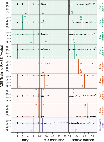
Appendix Figure. Results from the tuneRanger hyperparameter tuning operation. For each of the nine models (four environmental cluster models, four species composition cluster models, and one range-wide model), three hyperparameters were tuned, including the number of predictors evaluated at each decision tree split (mtry), the smallest number of samples in a decision tree’s terminal node (min.node.size), and the proportion of data from which a decision tree sample was built (sample.fraction). For all plots, the y-axis represents the training out-of-bag predictive error, measured as RMSE in Mg/ha. The points represent each of the 100 iterations tuneRanger runs. The dashed line represents a generalized additive model, highlighting the smoothed trend between predictive error and hyperparameter. The vertical solid line and associated numerical value represent the hyperparameter value that was selected.

References

- Ahlström, A., M. R. Raupach, G. Schurgers, B. Smith, A. Arneth, M. Jung, M. Reichstein, et al. 2015. “Carbon Cycle. The Dominant Role of Semi-Arid Ecosystems in the Trend and Variability of the Land CO₂ Sink.” Science 348 (6237): 895–24. https://doi.org/10.1126/SCIENCE.AAA1668.
- Anderegg, W. R. L., J. A. Hicke, R. A. Fisher, C. D. Allen, J. Aukema, B. Bentz, S. Hood, et al. 2015. “Tree Mortality from Drought, Insects, and Their Interactions in a Changing Climate.” New Phytologist 208 (3): 674–683. https://doi.org/10.1111/nph.13477.
- Ayrey, E., D. J. Hayes, S. Fraver, J. A. Kershaw, and A. R. Weiskittel. 2019. “Ecologically-Based Metrics for Assessing Structure in Developing Area-Based, Enhanced Forest Inventories from LiDAR.” Canadian Journal of Remote Sensing 45 (1): 88–112. https://doi.org/10.1080/07038992.2019.1612738.
- Blackburn, R. C., R. Buscaglia, and A. J. Sánchez Meador. 2021. “Mixtures of Airborne Lidar-Based Approaches Improve Predictions of Forest Structure.” Canadian Journal of Forest Research 51 (8): 1106–1116. https://doi.org/10.1139/cjfr-2020-0506.
- Breiman, L. 2001. “Random Forests.” Machine Learning 45 (1): 5–32. https://doi.org/10.1023/A:1010933404324.
- Breshears, D. D., N. S. Cobb, P. M. Rich, K. P. Price, C. D. Allen, R. G. Balice, W. H. Romme, et al. 2005. “Regional Vegetation Die-Off in Response to Global-Change-Type Drought.” Proceedings of the National Academy of Sciences 102 (42): 15144–15148. https://doi.org/10.1073/pnas.0505734102.
- Campbell, M. J., P. E. Dennison, K. L. Kerr, S. C. Brewer, and W. R. L. Anderegg. 2021. “Scaled Biomass Estimation in Woodland Ecosystems: Testing the Individual and Combined Capacities of Satellite Multispectral and Lidar Data.” Remote Sensing of Environment 262 (12511): 112511. https://doi.org/10.1016/j.rse.2021.112511.
- Campbell, M. J., P. E. Dennison, J. W. Tune, S. A. Kannenberg, K. L. Kerr, B. F. Codding, and W. R. L. Anderegg. 2020. “A Multi-Sensor, Multi-Scale Approach to Mapping Tree Mortality in Woodland Ecosystems.” Remote Sensing of Environment 245:111853. https://doi.org/10.1016/J.RSE.2020.111853.
- Campbell, M. J., and J. F. Eastburn. 2024. “Piñon-Juniper Woodland Species-Based Plot-Level Aboveground Biomass Dataset [ dataset]. https://doi.org/10.17605/OSF.IO/8Q9Y5.
- Campbell, M. J., J. F. Eastburn, K. A. Mistick, A. M. Smith, and A. E. L. Stovall. 2023. “Mapping Individual Tree and Plot-Level Biomass Using Airborne and Mobile Lidar in piñon-Juniper Woodlands.” International Journal of Applied Earth Observation and Geoinformation 118 (103232): 103232. https://doi.org/10.1016/j.jag.2023.103232.
- Cao, L., J. Pan, R. Li, J. Li, and Z. Li. 2018. “Integrating Airborne LiDAR and Optical Data to Estimate Forest Aboveground Biomass in Arid and Semi-Arid Regions of China.” Remote Sensing 10 (4): 532. https://doi.org/10.3390/rs10040532.
- Chave, J., R. Condit, S. Aguilar, A. Hernandez, S. Lao, R. Perez, Y. Malhi, and O. L. Phillips. 2004. “Error Propagation and Sealing for Tropical Forest Biomass Estimates.” Philosophical Transactions of the Royal Society B: Biological Sciences 359 (1443): 409–420. https://doi.org/10.1098/rstb.2003.1425.
- Chave, J., S. Davies, O. Phillips, S. Lewis, P. Sist, D. Schepaschenko, J. Armston, T. Baker, D. Coomes, and M. Disney. 2019. “Ground Data Are Essential for Biomass Remote Sensing Missions.” Surveys in Geophysics 40 (4): 863–880. https://doi.org/10.1007/s10712-019-09528-w.
- Chen, L., C. Ren, G. Bao, B. Zhang, Z. Wang, M. Liu, W. Man, and J. Liu. 2022. “Improved Object-Based Estimation of Forest Aboveground Biomass by Integrating LiDAR Data from GEDI and ICESat-2 with Multi-Sensor Images in a Heterogeneous Mountainous Region.” Remote Sensing 14 (12): 2743. https://doi.org/10.3390/rs14122743.
- Chojnacky, D. C., L. S. Heath, and J. C. Jenkins. 2014. “Updated Generalized Biomass Equations for North American Tree Species.” Forestry 87 (1): 129–151. https://doi.org/10.1093/forestry/cpt053.
- Chojnacky, D. C., and P. Rogers. 1999. “Converting Tree Diameter Measured at Root Collar to Diameter at Breast Height.” Western Journal of Applied Forestry 14 (1): 14–16. https://doi.org/10.1093/wjaf/14.1.14.
- Core Team, R. 2021. “R: A Language and Environment for Statistical Computing.” Computer Software. R Foundation for Statistical Computing, Vienna, Austria.https://www.R-project.org/.
- Cunliffe, A. M., C. D. McIntire, F. Boschetti, K. J. Sauer, M. Litvak, K. Anderson, and R. E. Brazier. 2020. “Allometric Relationships for Predicting Aboveground Biomass and Sapwood Area of Oneseed Juniper (Juniperus Monosperma) Trees.” Frontiers in Plant Science 11:94. https://doi.org/10.3389/fpls.2020.00094.
- Cutler, D. R., T. C. Edwards, K. H. Beard, A. Cutler, K. T. Hess, J. Gibson, and J. J. Lawler. 2007. “Random Forests for Classification in Ecology.” Ecology 88 (11): 2783–2792. https://doi.org/10.1890/07-0539.1.
- Dubayah, R., J. B. Blair, S. Goetz, L. Fatoyinbo, M. Hansen, S. Healey, M. Hofton, et al. 2020. “The Global Ecosystem Dynamics Investigation: High-Resolution Laser Ranging of the Earth’s Forests and Topography.” Science of Remote Sensing: 1(1000022. https://doi.org/10.1016/j.srs.2020.100002.
- Eisfelder, C., C. Kuenzer, and S. Dech. 2012. “Derivation of Biomass Information for Semi-Arid Areas Using Remote-Sensing Data.” International Journal of Remote Sensing 33 (9): 2937–2984. https://doi.org/10.1080/01431161.2011.620034.
- Ernst-Brock, C., L. Turner, R. J. Tausch, and E. A. Leger. 2019. “Long-Term Vegetation Responses to Pinyon-Juniper Woodland Reduction Treatments in Nevada, USA.” Journal of Environmental Management 242:315–326. https://doi.org/10.1016/j.jenvman.2019.04.053.
- Fekety, P. A., M. J. Falkowski, A. T. Hudak, T. B. Jain, and J. S. Evans. 2018. “Transferability of Lidar-Derived Basal Area and Stem Density Models within a Northern Idaho Ecoregion.” Canadian Journal of Remote Sensing 44 (2): 131–143. https://doi.org/10.1080/07038992.2018.1461557.
- Filippelli, S. K., M. J. Falkowski, A. T. Hudak, P. A. Fekety, J. C. Vogeler, A. H. Khalyani, B. M. Rau, and E. K. Strand. 2020. “Monitoring Pinyon-Juniper Cover and Aboveground Biomass Across the Great Basin.” Environmental Research Letters 15 (2): 025004. https://doi.org/10.1088/1748-9326/AB6785.
- Flake, S. W., and P. J. Weisberg. 2019. “Fine‐Scale Stand Structure Mediates Drought‐Induced Tree Mortality in Pinyon–Juniper Woodlands.” Ecological Applications 29 (2): e01831. https://doi.org/10.1002/eap.1831.
- Floyd, M. L., D. D. Hanna, and W. H. Romme. 2004. “Historical and Recent Fire Regimes in Piñon-Juniper Woodlands on Mesa Verde, Colorado, USA.” Forest Ecology and Management 198 (1–3): 269–289. https://doi.org/10.1016/j.foreco.2004.04.006.
- Gaylord, M. L., T. E. Kolb, W. T. Pockman, J. A. Plaut, E. A. Yepez, A. K. Macalady, R. E. Pangle, and N. G. Mcdowell. 2013. “Drought Predisposes piñon–Juniper Woodlands to Insect Attacks and Mortality.” New Phytologist 198 (2): 567–578. https://doi.org/10.1111/NPH.12174.
- Genuer, R., J.-M. Poggi, and C. Tuleau-Malot. 2015. VSURF: An R Package for Variable Selection Using Random Forests. http://CRAN.R-project.org/package=VSURF.
- Gleason, C. J., and J. Im. 2012. “Forest Biomass Estimation from Airborne LiDAR Data Using Machine Learning Approaches.” Remote Sensing of Environment 125:80–91. https://doi.org/10.1016/j.rse.2012.07.006.
- Greenwood, D. L., and P. J. Weisberg. 2008. “Density-Dependent Tree Mortality in Pinyon-Juniper Woodlands.” Forest Ecology and Management 255 (7): 2129–2137. https://doi.org/10.1016/j.foreco.2007.12.048.
- Grier, C. C., K. J. Elliott, and D. G. McCullough. 1992. “Biomass Distribution and Productivity ofPinus Edulis—Juniperus Monosperma Woodlands of North-Central Arizona.” Forest Ecology and Management 50 (3–4): 331–350. https://doi.org/10.1016/0378-1127(92)90346-B.
- Grüner, E., T. Astor, and M. Wachendorf. 2021. “Prediction of Biomass and N Fixation of Legume–Grass Mixtures Using Sensor Fusion.” Frontiers in Plant Science 11:603921. https://doi.org/10.3389/fpls.2020.603921.
- Huang, C. Y., G. P. Asner, R. E. Martin, N. N. Barger, and J. C. Neff. 2009. “Multiscale Analysis of Tree Cover and Aboveground Carbon Stocks in Pinyon–Juniper Woodlands.” Ecological Applications 19 (3): 668–681. https://doi.org/10.1890/07-2103.1.
- Huffman, D. W., P. Z. Fulé, J. E. Crouse, and K. M. Pearson. 2009. “A Comparison of Fire Hazard Mitigation Alternatives in Pinyon–Juniper Woodlands of Arizona.” Forest Ecology and Management 257 (2): 628–635. https://doi.org/10.1016/j.foreco.2008.09.041.
- Huffman, D. W., M. T. Stoddard, J. D. Springer, J. E. Crouse, A. J. Sánchez Meador, and S. Nepal. 2019. “Stand Dynamics of Pinyon-Juniper Woodlands After Hazardous Fuels Reduction Treatments in Arizona.” Rangeland Ecology & Management 72 (5): 757–767. https://doi.org/10.1016/j.rama.2019.05.005.
- Isenburg, M. 2006. “LAStools—Efficient LiDAR Processing Software (No. 211112).” Computer Software.
- Jacobs B. F. 2008. “Southwestern, U.S. juniper savanna and pinon-juniper woodland communities: Ecological history and natural range of variability“ In Ecology, Management, and Restoration of Pinon-Juniper and Ponderosa Pine Ecosystems: Combined Proceedings of the 2005 St. George Utah and 2006 Albuquerque, Albuquerque, NM, USA; New Mexico Workshops, St. George, UT, USA. Proceedings RMRS-P-51, edited by G. J. Gottfried, J. D. Shaw, and P. L. Ford, 11–19. Fort Collins, CO, USA: US Deparatment of Agriculture, Forest Service, Rocky Mountain Research Station.
- Jain, A. K. 2010. “Data Clustering: 50 Years Beyond K-Means.” Pattern Recognition Letters 31 (8): 651–666. https://doi.org/10.1016/j.patrec.2009.09.011.
- Jenkins, J. C., D. C. Chojnacky, L. S. Heath, and R. A. Birdsey. 2003. “National-Scale Biomass Estimators for United States Tree Species.” Forest Science 49 (1): 12–35. https://doi.org/10.1093/forestscience/49.1.12.
- Jiang, J., Y. Shu, J. Wang, and M. Long. 2022. “Transferability in Deep Learning: A Survey.” https://doi.org/10.48550/ARXIV.2201.05867.
- Kannenberg, S. A., A. W. Driscoll, D. Malesky, and W. R. L. Anderegg. 2021. “Rapid and Surprising Dieback of Utah Juniper in the Southwestern USA Due to Acute Drought Stress.” Forest Ecology and Management 480 (118639): 118639. https://doi.org/10.1016/j.foreco.2020.118639.
- Krofcheck, D. J., M. E. Litvak, C. D. Lippitt, and A. Neuenschwander. 2016. “Woody Biomass Estimation in a Southwestern U.S. Juniper Savanna Using LiDAR-Derived Clumped Tree Segmentation and Existing Allometries.” Remote Sensing 8 (6): 453. https://doi.org/10.3390/RS8060453.
- LANDFIRE. 2020. LANDFIRE Remap 2016 Existing Vegetation Type (EVT) CONUS [ dataset]. https://landfire.gov/evt.php.
- Lefsky, M. A., W. B. Cohen, G. G. Parker, and D. J. Harding. 2002. “Lidar Remote Sensing for Ecosystem Studies.” BioScience 52 (1): 19–30. https://doi.org/10.1641/0006-3568(2002)052[0019:LRSFES]2.0.CO;2.
- Magargal, K., K. Wilson, S. Chee, M. J. Campbell, V. Bailey, P. E. Dennison, W. R. L. Anderegg, A. Cachelin, S. Brewer, and B. F. Codding. 2023. “The Impacts of Climate Change, Energy Policy and Traditional Ecological Practices on Future Firewood Availability for Diné (Navajo) People.” Philosophical Transactions of the Royal Society B: Biological Sciences 378 (1889): 20220394. https://doi.org/10.1098/rstb.2022.0394.
- McIntire, C. D., A. M. Cunliffe, F. Boschetti, K. J. Sauer, M. Litvak, K. Anderson, and R. E. Brazier. 2022. “Allometric Relationships for Predicting Aboveground Biomass, Sapwood, and Leaf Area of Two-Needle Piñon Pine (Pinus edulis) Amid Open-Grown Conditions in Central New Mexico.” Forest Science 68 (2): 152–161. https://doi.org/10.1093/forsci/fxac001.
- McTague, J. P., and A. Weiskittel. 2021. “Evolution, History, and Use of Stem Taper Equations: A Review of Their Development, Application, and Implementation.” Canadian Journal of Forest Research 51 (2): 210–235. https://doi.org/10.1139/cjfr-2020-0326.
- Miller, R. F., J. C. Chambers, L. Evers, C. J. Williams, K. A. Snyder, B. A. Roundy, and F. B. Pierson. 2019. “The Ecology, History, Ecohydrology, and Management of Pinyon and Juniper Woodlands in the Great Basin and Northern Colorado Plateau of the Western United States.” United States Department of Agriculture, Forest Service: RMRS-GTR-403. https://doi.org/10.2737/RMRS-GTR-403.
- Miller, E. L., R. O. Meeuwig, and J. D. Budy. 1981. Biomass of Singleleaf Pinyon and Utah Juniper (INT-RP-273). U.S. Department of Agriculture, Forest Service, Intermountain Forest and Range Experiment Station. https://doi.org/10.2737/INT-RP-273.
- Miller, R. F., R. J. Tausch, E. D. Mcarthur, D. D. Johnson, and S. C. Sanderson. 2008. “Age Structure and Expansion of Piñon-Juniper Woodlands: A Regional Perspective in the Intermountain West.” United States Department of Agriculture, Forest Service: RMRS-RP-69. https://doi.org/10.2737/RMRS-RP-69.
- Muldavin, E., and F. J. Triepke. 2020. “North American Pinyon-Juniper Woodlands: Ecological Composition, Dynamics, and Future Trends.” InEncyclopedia of the World’s Biomes, edited by M. I. Goldstein and D. A. DellaSella, 516–531. https://doi.org/10.1016/B978-0-12-409548-9.12113-X.
- Neeti, N., and R. Kennedy. 2016. “Comparison of National Level Biomass Maps for Conterminous US: Understanding Pattern and Causes of Differences.” Carbon Balance and Management 11 (1): 19. https://doi.org/10.1186/s13021-016-0060-y.
- PRISM Climate Group at Oregon State University. 2022). [ dataset] https://prism.oregonstate.edu.
- Probst, P., M. N. Wright, and A.-L. Boulesteix. 2018. “Hyperparameters and Tuning Strategies for Random Forest.” Wiley Interdisciplinary Reviews: Data Mining and Knowledge Discovery 9 (3): e1301. https://doi.org/10.1002/widm.1301.
- Randin, C. F., T. Dirnböck, S. Dullinger, N. E. Zimmermann, M. Zappa, and A. Guisan. 2006. “Are Niche-Based Species Distribution Models Transferable in Space?” Journal of Biogeography 33 (10): 1689–1703. https://doi.org/10.1111/j.1365-2699.2006.01466.x.
- Redmond, M. D., N. S. Cobb, M. E. Miller, and N. N. Barger. 2013. “Long-Term Effects of Chaining Treatments on Vegetation Structure in piñon-Juniper Woodlands of the Colorado Plateau.” Forest Ecology and Management 305:120–128. https://doi.org/10.1016/j.foreco.2013.05.020.
- Riley, K. L., I. C. Grenfell, M. A. Finney, and J. M. Wiener. 2021. “TreeMap, a Tree-Level Model of Conterminous US Forests Circa 2014 Produced by Imputation of FIA Plot Data.” Scientific Data 8 (1): 11. https://doi.org/10.1038/s41597-020-00782-x.
- Romme, W. H., C. D. Allen, J. D. Bailey, W. L. Baker, B. T. Bestelmeyer, P. M. Brown, K. S. Eisenhart, et al. 2009. “Historical and Modern Disturbance Regimes, Stand Structures, and Landscape Dynamics in piñon-Juniper Vegetation of the Western United States.” Rangeland Ecology and Management 62 (3): 203–222. https://doi.org/10.2111/08-188R1.1.
- Roussel, J. R., and D. Auty. 2023. Airborne LiDAR Data Manipulation and Visualization for Forestry Applications. R package version 4.0.3. https://cran.r-project.org/package=lidR.
- Roussel, J. R., D. Auty, N. C. Coops, P. Tompalski, T. R. H. Goodbody, A. S. Meador, J. F. Bourdon, F. D. Boissieu, and A. Achim. 2020. “LidR: An R Package for Analysis of Airborne Laser Scanning (ALS) Data.” Remote Sensing of Environment 251 (112061): 112061. https://doi.org/10.1016/j.rse.2020.112061.
- Saarela, S., A. Wästlund, E. Holmström, A. A. Mensah, S. Holm, M. Nilsson, J. Fridman, and G. Ståhl. 2020. “Mapping Aboveground Biomass and Its Prediction Uncertainty Using LiDAR and Field Data, Accounting for Tree-Level Allometric and LiDAR Model Errors.” Forest Ecosystems 7 (1): 1–17. https://doi.org/10.1186/s40663-020-00245-0.
- Sankey, T., R. Shrestha, J. B. Sankey, S. Hardegree, and E. Strand. 2013. “Lidar-Derived Estimate and Uncertainty of Carbon Sink in Successional Phases of Woody Encroachment.” Journal of Geophysical Research: Biogeosciences 118 (3): 1144–1155. https://doi.org/10.1002/JGRG.20088.
- Sequeira, A. M. M., P. J. Bouchet, K. L. Yates, K. Mengersen, M. J. Caley, and J. McPherson. 2018. “Transferring Biodiversity Models for Conservation: Opportunities and Challenges.” Methods in Ecology and Evolution 9 (5): 1250–1264. https://doi.org/10.1111/2041-210X.12998.
- Shaw, J. D., B. E. Steed, and L. T. Deblander. 2005. “Forest Inventory and Analysis (FIA) Annual Inventory Answers the Question: What Is Happening to Pinyon-Juniper Woodlands?” Journal of Forestry 103 (6): 280–285. https://doi.org/10.1093/jof/103.6.280.
- Smith, W. K., M. P. Dannenberg, D. Yan, S. Herrmann, M. L. Barnes, G. A. Barron-Gafford, J. A. Biederman, et al. 2019. “Remote Sensing of Dryland Ecosystem Structure and Function: Progress, Challenges, and Opportunities.” Remote Sensing of Environment 233 (111401): 111401. https://doi.org/10.1016/j.rse.2019.111401.
- Sprinkle, W., and J. Klepac. 2015. “Models of Utah Juniper and Two-Needle Pinyon Biomass for One Site in Southwest Utah.” Forest Science 61 (1): 162–168. https://doi.org/10.5849/forsci.12-541.
- Sugarbaker, L. J., E. W. Constance, H. K. Heidemann, A. L. Jason, V. Lukas, D. L. Saghy, and J. M. Stoker. 2014. “The 3D Elevation Program Initiative—A Call for Action: Geological Survey Circular 1399.” https://doi.org/10.3133/cir1399.
- Tenneson, K., M. Patterson, T. Mellin, M. Nigrelli, P. Joria, and B. Mitchell. 2018. “Development of a Regional Lidar-Derived Above-Ground Biomass Model with Bayesian Model Averaging for Use in Ponderosa Pine and Mixed Conifer Forests in Arizona and New Mexico, USA.” Remote Sensing 10 (3): 442. https://doi.org/10.3390/rs10030442.
- Torre-Tojal, L., A. Bastarrika, A. Boyano, J. M. Lopez-Guede, and M. Graña. 2022. “Above-Ground Biomass Estimation from LiDAR Data Using Random Forest Algorithms.” Journal of Computational Science 58:101517. https://doi.org/10.1016/J.JOCS.2021.101517.
- Wager, S., T. Hastie, and B. Efron. 2014. “Confidence Intervals for Random Forests: The Jackknife and the Infinitesimal Jackknife.” Journal of Machine Learning Research 15 (1): 1625–1651.
- Wallach, D., and M. Genard. 1998. “Effect of Uncertainty in Input and Parameter Values on Model Prediction Error.” Ecological Modelling 105 (2–3): 337–345. https://doi.org/10.1016/S0304-3800(97)00180-4.
- Wenger, S. J., and J. D. Olden. 2012. “Assessing Transferability of Ecological Models: An Underappreciated Aspect of Statistical Validation.” Methods in Ecology and Evolution 3 (2): 260–267. https://doi.org/10.1111/J.2041-210X.2011.00170.X.
- Westfall, J. A., J. W. Coulston, A. N. Gray, J. D. Shaw, P. J. Radtke, D. M. Walker, A. R. Weiskittel, et al. 2023. A National-Scale Tree Volume, Biomass, and Carbon Modeling System for the United States (WO-GTR-104). U.S. Department of Agriculture, Forest Service. https://doi.org/10.2737/WO-GTR-104.
- Westfall, J. A., and C. W. Woodall. 2007. “Measurement Repeatability of a Large-Scale Inventory of Forest Fuels.” Forest Ecology and Management 253 (1–3): 171–176. https://doi.org/10.1016/j.foreco.2007.07.014.
- Williams, A. P., B. I. Cook, and J. E. Smerdon. 2022. “Rapid Intensification of the Emerging Southwestern North American Megadrought in 2020–2021.” Nature Climate Change 12 (3): 232–234. https://doi.org/10.1038/s41558-022-01290-z.
- Wright, M. N., and A. Ziegler. 2017. “Ranger: A Fast Implementation of Random Forests for High Dimensional Data in C++ and R.” Journal of Statistical Software 77 (1): 1–17. https://doi.org/10.18637/jss.v077.i01.
- Wu, Z., D. Dye, J. Vogel, and B. Middleton. 2016. “Estimating Forest and Woodland Aboveground Biomass Using Active and Passive Remote Sensing.” Photogrammetric Engineering and Remote Sensing 82 (4): 271–281. https://doi.org/10.14358/PERS.82.4.271.
- Yates, K. L., P. J. Bouchet, M. J. Caley, K. Mengersen, C. F. Randin, S. Parnell, A. H. Fielding, et al. 2018. “Outstanding Challenges in the Transferability of Ecological Models.” Trends in Ecology and Evolution 33 (10): 790–802. https://doi.org/10.1016/J.TREE.2018.08.001.
- Zhang, G., and Y. Lu. 2012. “Bias-Corrected Random Forests in Regression.” Journal of Applied Statistics 39 (1): 151–160. https://doi.org/10.1080/02664763.2011.578621.