Synthesis and evaluation of seamless, large-scale, multispectral satellite images using Generative Adversarial Networks on land use and land cover and Sentinel-2 data

ABSTRACT

Artificial intelligence (AI) began to make its way into geoinformation science several decades ago and since then has constantly brought forth new cutting-edge approaches for diverse geographic use cases. AI and deep learning methods have become essential approaches for land use and land cover (LULC) classifications, which are important in urban planning and regional management. While the extraction of LULC information from multispectral satellite images has been a well-studied part of past and present research, only a few studies emerged about the recovery of spectral properties from LULC information. Estimates of the spectral characteristics of LULC categories could enrich LULC forecasting models by providing necessary information to delineate vegetation indices or microclimatic parameters. We train two identical Conditional Generative Adversarial Networks (CGAN) to synthesize a multispectral Sentinel-2 image based on different combinations of open-source LULC data sets. Large-scale synthetic multispectral satellite images of the administrative region of Bonn and Rhein-Sieg in Germany are generated with a Euclidean distance-based patch-fusion method. The approach generated a realistic-looking satellite image without noticeable seams between patch borders. Based on several metrics, such as difference calculations, the spectral information divergence (SID), and the Fréchet inception distance (FID), we evaluate the resulting images. The models reach mean SIDs as low as 0.026 for urban fabrics and forests and FIDs below 90 for bands B2 and B5 showing that the CGAN is capable of synthesizing distinct synthetic features matching with features typical for respective LULC categories and manages to mimic multispectral signatures. The method used in this paper to generate large-scale synthetic multispectral satellite images can be used as an approach to support scenario-oriented sustainable urban planning.

KEYWORDS:

• Synthetic satellite images
• Generative Adversarial Network
• Sentinel-2
• patch fusion
• Deep Fake Geography

1. Introduction

Artificial Intelligence (AI) constantly brings forth new cutting-edge approaches for diverse geographic use cases, such as traffic monitoring, urban planning, or building stock extraction (Zhao et al. 2021; Couclelis 1986; Adegun, Viriri, and Tapamo 2023; Mandal et al. 2020; Dongjie; Wang, Lu, and Fu 2022; Wurm et al. 2021). Today, AI tools and associated Deep Learning (DL) packages are easily accessible through several frameworks that even got integrated into Geographic Information Systems (GIS) (ESRI 2020). Object detection (Lang et al. 2021; Z. Li et al. 2022) and image classification, in the broader sense, with semantic segmentation (Y. Liu et al. 2017; Lu et al. 2021; Lv et al. 2023; Wurm et al. 2021) and instance segmentation (Gong et al. 2022; Yang et al. 2021) as more specific approaches emerged from the field of Computer Vision (CV) (Lv et al. 2023) but are extensively used in remote sensing and the derivation of corresponding products. With an essential role in urban planning and regional management, land use and land cover (LULC) data sets are among such products and can be derived using DL methods (Cai et al. 2019; Campos-Taberner et al. 2020). While the extraction of LULC information from multispectral satellite images is a well-studied part of past and present research, the recovery of spectral properties from LULC information has hardly been investigated. However, estimates of the spectral characteristics of LULC categories could enrich the information content of LULC forecasting models and support scenario-oriented urban planning. This paper will explore the potential of a Conditional Generative Adversarial Network (CGAN) for synthesizing such spectral signatures based on open-source LULC information. As one of the most popular generative DL methods, Generative Adversarial Networks (GANs) were found to offer great applicability in many fields of geoscience due to the large available number of data sets to learn from (Mateo-García et al. 2021). GANs were first mentioned by Goodfellow et al. (2014) and are used to generate new data similar to a given training data set using two adversarial networks, usually referred to as generator and discriminator. In general, the generator seeks to deceive the discriminator by giving it synthetic data which is meant to be indistinguishable from the original data. Besides this synthetic data, the discriminator also receives the original data and tries to identify whether the data is real or fake. During the training process, both networks are trained simultaneously against each other (Foster 2020). The first GANs were used to be unsupervised in a manner that the generator only received a random noise vector as an input from which to generate data. The discriminator then tries to distinguish between original and generated images, as mentioned before (Mateo-García et al. 2021). Shortly thereafter, CGANs were developed using an additional feature vector beside or instead of the random noise vector as a generator’s input. The additional input enables the generator to create tailored synthetic data according to the feature vector’s specification but poses the need for paired training data (Mirza and Osindero 2014). Addressing the lack of paired training data for some domains, Isola et al. (2017) developed a Cycle-consistent Generative Adversarial Network (CycleGAN), which manages unpaired image-to-image translation.

In the field of geosciences and especially remote sensing, GANs are deployed for various applications, such as domain adaption (Benjdira et al. 2019; Ji, Wang, and Luo 2021; Soto et al. 2020), change detection (C. He et al. 2022; Hou et al. 2020; Lebedev et al. 2018) and super-resolution (B. Liu et al. 2021; Zhu et al. 2023). However, GANs have also opened up the entirely new field of “Deep Fake Geography,” as it has been coined by B. Zhao et al. (2021) to emphasize the impact of AI on the challenges of erroneous or simplified geospatial data inherent in geography. The authors trained a CycleGAN proposed by Isola et al. (2017), to translate between topographic base maps and Google Earth’s satellite images. Applying the trained model on unseen topographic maps, they created fake red-green-blue (RGB) satellite images to examine methods for detecting such deep-faked images. The CycleGAN managed to generate satellite images with an authentic visual appearance, even though all proposed methods for deep fake detection managed to identify more than 94% of the synthetic satellite images. Even though B. Zhao et al. (2021) brought up the term “Deep Fake Geography,” the authors were not the first to investigate the translation between different data domains. Y. Zhang et al. (2020) investigated the translation of satellite images into topographic base maps, in other words, the inverted approach of B. Zhao et al. (2021), using several GAN architectures based on Pix2Pix and CycleGAN. To reduce noise in the generated images, they enriched the generator’s input data with public GPS data and segmented derivatives of the satellite image. The semantic information originates from a second U-Net generator preceding the actual generator. Even though the combination of satellite images, semantic information, and Global Positioning System (GPS) data improved the generated road maps compared to the other tested architectures, none of the models generated realistic images. Focusing on the same translation problem, a powerful GAN architecture for satellite-to-map translation, called MapGAN, was proposed by J. Li et al. (2020). The model can produce several maps of different styles based on satellite images and auxiliary information referred to as render metrics that are given into the model. This one-to-many translation is made possible by a pre-trained classifier deployed beside the generator and the discriminator. The authors define the generator’s loss term as a combination of a feature render loss, a map classification loss, a perceptual loss, and an adversarial loss and claim that MapGAN outperforms several other state-of-the-art networks.

The feasibility of generating building footprints based on road network maps or land use data was demonstrated by A. N. Wu and Biljecki (2022) using a CGAN. They found that color-coded RGB road map data contributes to a reduction of artifacts in generated images compared to single-band gray scale input data. They applied their model, referred to as GANmapper, to nine cities and received visually compelling results. However, they highlighted the model’s sensibility to the selected zoom level for the training data.

Further application domains, which can also be associated with Deep Fake Geography, are the seasonal and land cover transfer of satellite images and local image splicing. Abady et al. (2020) deployed a NICE-GAN on RGB and near-infrared (NIR) channels of Sentinel-2 (S2) images to translate images of barren land cover into vegetated land cover. While the transfer from vegetated to barren land delivered satisfactory results, the transfer from barren to vegetated land showed deficits in the approach. However, the ProGAN and the NICE-GAN approaches were only validated on a few selected samples. Later, Abady et al. (2022) investigated both full satellite image modification of RGB plus near-infrared (NIR) S2 images and local splicing within RGB S2 images. For the former, they investigated the seasonal transfer between winter and summer images using a Pix2Pix model due to the existence of paired data for this transformation problem. Besides the seasonal transfer, they examined land cover transfer, turning images with dense vegetation into barren landscapes and vice versa using a CycleGAN due to the task’s nature of non-existent paired training data. Regarding local image splicing, the authors used an image generative pre-trained transformer and a vision transformer to fill in partially masked RGB images from the SEN12MS data set. In addition to their investigations about land cover translation, Abady et al. (2020) generated fake Sentinel-2 (S2) images from latent vectors using a ProGAN architecture trained on the SEN12MS data set (Schmitt et al. 2019). They claim to be the first authors using a GAN for multispectral synthetic satellite image generation using 13 bands of S2 and report good results regarding visual authenticity and multispectral properties. However, the approach was only validated on a few selected samples.

Even though several studies have used GANs on remote sensing data, just a few focus on the generation of synthetic satellite data, and the prospects of multispectral image generation have been neither widely investigated nor evaluated in depth, since impartial metrics have not been applied. Furthermore, the usage of LULC information as conditional GAN inputs has, to our knowledge, not been tested but can serve as an essential parameter to receive tailored results, opening new fields of applicability for LULC forecasting models and in scenario-based urban planning. As previous studies have proven, generating realistic patches of satellite images with GANs is possible. However, generating small square image patches only offers a few application possibilities, which raises the need for image stitching methods. This research aims to generate seamless, large-scale, synthetic multispectral satellite images that are supposed to mimic those captured by S2. In this context, we want to address the questions [i] whether open-source LULC data can be an adequate input for a CGAN to generate images with features corresponding to the underlying LULC classes, [ii] whether multispectral properties can be reliably synthesized by a CGAN and [iii] whether the CGAN’s performance differs between different LULC classes and [iv] between the image channels. We will investigate those questions using two training datasets from several federal states in western Germany that differ in terms of the amount of LULC information provided as inputs for the CGAN. The models will be evaluated based on unseen data from the administrative region of Bonn and Rhein-Sieg in Germany.

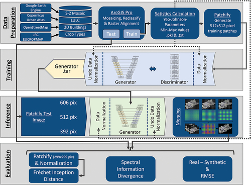
Subsequently, this paper will explain the methodology, including data preparation, data normalization, the model architecture, post-processing measures, and the applied evaluation. We will present the results, followed by their discussion, before we make concluding remarks.

2. Methodology

2.1. Data preparation

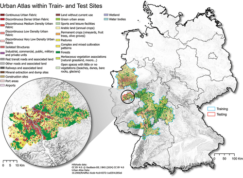
The training and validation data sets contain open-source data from different providers. We will refer to the data sets passed into the generator as input data and the data we are trying to replicate as target data. Spatially independent input and target data sets were created for training and testing. Training data were collected from various administrative districts in western Germany (cf. Figure 1). Due to its spatial proximity to the training sites and its diverse land use in proportion to its relatively small area, we tested the model on the administrative unit of Bonn and the surrounding Rhein-Sieg region, as illustrated in Figure 1.

Figure 1. Map of training and testing sites in Germany.

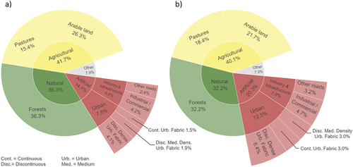
Two different sets of input data were used to train the network. The first input data set uses information from the Urban Atlas, a LULC product developed under the Copernicus Project, building footprints as vector files from OpenStreetMap and a no-data mask (European Commission 2020; European Environment Agency 2020). We will refer to this training data set as Training Set A. In addition to the inputs used in Training Set A, Training Set B uses crop-type information from the European Union Crop-Type Map provided by the Joint Research Centre of the European Commission (JRC 2021). The additional crop-type information is supposed to enhance the synthetic satellite image, assuming that it can assist the model in understanding agricultural land cover patterns. The crop type data set differentiates between several crop types that the Urban Atlas subsumes into a single class. Subsuming could result in the model’s inability to provide a differentiated picture for such vegetated areas. We trained a model for each training data set under identical architectures and will accordingly refer to these models as Model A and Model B. The land use classes from the Urban Atlas were reclassified into equal intervals of positive signed int16 values. No-data values were set to −32768 before rasterizing the vector file and resampling it onto the target satellite image. It must be mentioned that the Urban Atlas class 25,000 (orchards at the fringe of urban classes) is not represented in the training data set, and the classes 24,000 (complex and mixed cultivation patterns), 25000 (orchards at the fringe of urban classes) and 33,000 (open spaces with little or no vegetations, e.g. beaches, dunes, bare rocks, glaciers) are not present in the testing area and are thus not present in the testing data set. Nevertheless, we kept the classes as placeholders to ensure transferability during fine-tuning on other regions and did not set those classes to no-data values. The distribution of LULC classes is shown in Figure 2. The building footprint layer was also classified (building = max(signed int16), no building = min(signed int16)) and rasterized onto the target satellite image. The no-data mask was generated from the no-data regions in the Urban Atlas data set and inherited the analog classification scheme used for the building footprints. The crop-type data set is provided in raster data format and was aligned with the target satellite image and reclassified into equal intervals of positive signed int16 values, just like we did for the Urban Atlas land use classes. The Urban Atlas and the crop-type data were generated for 2018 (European Environment Agency 2020).

Figure 2. Distribution of class shares of land use and land cover in (a) training and (b) test area.

The target data contains the S2 Level-2A bands B2, B3, B4, B5, B6, B7, B8, B8A, B11 and B12. As suggested by Rosentreter, Hagensieker, and Waske (2020), C. Qiu et al. (2019), and C. Qiu et al. (2020), who worked on the application of S2 scenes to extract local climate zones, which we consider a potential field of application for synthetic images, we omitted bands 1 (coastal aerosol), 9 (water vapor) and 10 (SWIR – cirrus) due to their little contribution to such segmentation tasks. Image statistics of the selected channels are listed in Table 1. We created cloud-free mosaics within the bounds of the LULC data set using the Google Earth Engine (GEE) (Gorelick et al. 2017). In accordance with the input data’s year of acquisition, the mosaic contains S2 images from June to August 2018 and from the same months in 2017 and 2019 to fill in gaps. All bands were resampled to 10-meter spatial resolution.

Table 1. Image statistics of S2 training images.

	B2	B3	B4	B5	B6	B7	B8	B8A	B11	B12
mean	415,0	650,4	605,8	1071,4	2436,0	2975,0	3121,0	3246,4	1981,3	1167,6
median	360	631	481	1042	2477	3009	3182	3320	1910	1090
sd	289,0	333,9	468,1	463,9	568,9	749,0	827,8	800,8	615,3	557,8
min	1	1	1	1	1	1	1	1	32	14
max	18272	17280	16576	16282	16024	15888	15794	15726	15158	15103

Both input and target data were cut into square patches of several initial sizes (256, 320, 384, 448, 512, 576, 640, 704, 768, 832, 896, 960, 1024 pixels) that were resampled to 512 pixels if not already the case. The patches overlap between 25% and 50%, depending on their initial size. We allowed a no-data percentage of up to 50%. Each input patch contains 31 bands within Training Set A and 32 bands within Training Set B, including the grayscale crop-type band. The other bands are a binary no-data mask, binary building footprints, the Urban Atlas LULC as a grayscale, each LULC class as a binary representation, and a band with a constant value for the native patch size. Both training data sets contain roughly 30,000 image pairs.

2.2. Data normalization

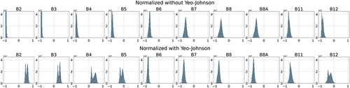
Considering the extensive value range for reflectance values in satellite images, normalizing the data becomes essential to minimize the model’s loss function efficiently. However, most land cover classes are not homogeneously distributed across the training area. For example, industrial parks, dense urban structures, or water bodies are spatially centered and are, therefore, not present in every training patch. Hence, we calculated the overall parameters for the normalization based on the whole images and not on the individual patches. While the input data consists of evenly distributed classes, the continuous target data contains several skewed channels, making it difficult to train the model. To reduce the skewness, we applied a Yeo-Johnson transformation on the target data preceding the actual data normalization. We calculated image statistics, such as Yeo – Johnson’s transformer parameters and the transformed minimum and maximum values of each channel of the target data, while considering the untransformed minimum and maximum values for the input data. Those statistics are based on the whole input and target images and are used within the model’s data loader to normalize each input and target patch. Hence, each patch is normalized just before being pushed through the model.

Within the data loader, the Yeo – Johnson transformation is applied on the target patch, followed by a rescaling and shifting to a value range between −0.95 and 0.95 with no data values being set to −1. Figure 3 shows the difference between the rescaled and shifted distributions of the satellite images with and without a prior Yeo – Johnson transformation.

Figure 3. Difference between scaled and shifted reflectance values with and without a prior Yeo-Johnson transformation.

Considering the categorical character of land cover information, we did not apply the Yeo – Johnson transformation to the input data but rescaled and shifted their distribution to a value range between − 0.95 and 0.95 with no data values set to −1 as represented in Formula 1(1) $\mathit{Norm}\left(x_{\mathit{i},\mathit{j}}\right)=\left\{\begin{array}{cc}\frac{{\mathit{x}}_{\mathit{i},\mathit{j}}-min\left(x_j\right)}{max\left(x_j\right)-min\left(x_j\right)}\ast 1.9-0.95& x_{\mathit{i},\mathit{j}}\ne \mathrm{\varnothing }\\ -1& x_{\mathit{i},\mathit{j}}=\mathrm{\varnothing }\end{array}\right.$(1) .

(1) $\mathit{Norm}\left(x_{\mathit{i},\mathit{j}}\right)=\left\{\begin{array}{cc}\frac{{\mathit{x}}_{\mathit{i},\mathit{j}}-min\left(x_j\right)}{max\left(x_j\right)-min\left(x_j\right)}\ast 1.9-0.95& x_{\mathit{i},\mathit{j}}\ne \mathrm{\varnothing }\\ -1& x_{\mathit{i},\mathit{j}}=\mathrm{\varnothing }\end{array}\right.$(1)

$x_{\mathit{i},\mathit{j}}$ is the pixel value at position i in channel j and $\mathrm{\varnothing }$ denotes the no-data value.

While the target data required more complex data normalization, the input data was just scaled into a value range between − 0.95 and 0.95 using the minimum and maximum values and no-data values were set to − 1.

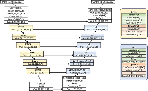
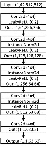
2.3. Model architecture

We adapted the concept and the rough architecture from the Pix2Pix network (Isola et al. 2016; Persson 2021). However, several changes to the architecture were made. The generator has a U-NET architecture with eight down- and up-sampling blocks and a skip connection between each corresponding block. Besides the first and last block in the downward part, each down-sampling block consists of an intermediate block, which only changes the depth of the tensor but keeps its height and width, followed by the actual down-sampling block, which reduces the width and height by a stride of two. Both parts of the down-sampling block use instance normalization and a leaky rectified linear unit. The upward part makes use of a similar structure, except for transposed convolutions and rectified linear unit activation functions. The last block uses a transposed convolution to retrieve the original width and height, followed by a convolution with an increased kernel size of eight-by-eight before a rectified hyperbolic tangent function (ReTanh) is applied. The ReTanh is intended to ensure that the value range of the normalized training satellite images is reconstructed by setting no-data pixels to −1 and valid pixels between −0.95 and 1. The function is defined as

(2) $\mathit{ReTanh}\left(\mathit{x}\right)=\left\{\begin{array}{cc}\tanh \left(\mathit{x}\right)& \tanh \left(\mathit{x}\right)\ge -0.95\\ -1& \tanh \left(\mathit{x}\right)<-0.95\end{array}\right.$(2)

Where tanh(x) is defined as

(3) $\tanh \left(\mathit{x}\right)=\frac{\exp \left(x\right)-\exp \left(-\mathit{x}\right)}{\exp \left(x\right)+\exp \left(-\mathit{x}\right)}$(3)

Figure 4 shows the architecture of the generator based on the input dimensions of Training Set B.

Figure 4. U-NET Architecture of the generator with downsampling and upsampling blocks and skip connections. In- and output dimensions are based on Training Set B input data. Kernel sizes are provided for convolutional layers.

The discriminator is a Patch GAN with a receptive field of 70 pixels and consists of five down-sampling convolutional layers with a stride of two, except for the last two convolutions, which only have a stride of one. Figure 5 illustrates the discriminator’s architecture.

Figure 5. PatchGAN Architecture of the discriminator within the CGAN. In- and output dimensions are based on Training Set B input data. Kernel sizes are provided for convolutional layers.

We combined a Binary Cross-Entropy (BCE) and an L1 loss function and applied an Adam solver, as suggested by Isola et al. (2016). The BCE is calculated on the discriminator’s output and added to the L1 loss, which is multiplied by a constant of 100. Addressing the issue of an unstable training process, we used different learning rates for the adversarial networks, using 4.05E–05 for the generator and 2.02E–05 for the discriminator in combination with exponential learning rate schedulers driven by a γ of 0.99. We tested over 40 versions of the model architecture under different hyperparameters and manually compared the results during training. The tendency of GANs to exhibit training instability, mode collapse, and vanishing gradients has led to the decision against employing automated hyperparameter tuning. We trained a CGAN on each training data set for 50 epochs (roughly 135 hours) on a server with an NVIDIA A40 (48GB) Graphics Processing Unit and 500 GB of Random Access Memory.

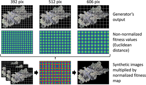
2.4. Post-processing – patch blending

Since the generation of simple square synthetic satellite images offers little added value for users, we have used the patch blending method suggested by Siracusa, Seychell, and Bugeja (2021) to create large-scale images within the model’s inference. Because of a GAN’s lack of awareness about adjacent patches, artifacts can occur on the edges of individual patches due to differently rendered objects. Therefore, we ran the validation inputs several times through the generator, each time using a different tile division to split the input image into patches. The exact size of the patches was calculated by the adjacent prime number divisors above and below the nearest prime number of the input image size divided by the original patch size (512 pixels). Thus, the input image was cut into the patch sizes of 392, 512, and 606 pixels in our use case. Prime numbers were used to calculate these values to avoid overlapping patch boundaries in the large-scale image. We will refer to the three cut images (by 392, 512, and 606 pixels) as tile layers. Each patch within each tile layer was filled with fitness values corresponding to the Euclidean distance from the center of each patch to its outer bounds, as illustrated in Figure 6. The fitness values are then normalized across the channels as shown in Formula 4(4) ${\mathit{\omega }}_{\left(\mathit{x},\mathit{y},\mathit{z}\right)}=\frac{{\mathrm{\Phi }}_{\left(\mathit{x},\mathit{y},\mathit{z}\right)}-\mathit{mi}{n}_{\mathrm{\Phi }\left(\mathit{x},\mathit{y},0\dots \mathit{n}-1\right)}}{\sum _{\mathit{z}=0}^{\mathit{n}-1}({\mathrm{\Phi }}_{\left(\mathit{x},\mathit{y},\mathit{z}\right)}-\mathit{mi}{n}_{\mathrm{\Phi }\left(\mathit{x},\mathit{y},0\dots \mathit{n}-1\right)})}$(4) , resulting in per-pixel sums of 1, while the lowest contributing fitness value was set to 0 (Siracusa, Seychell, and Bugeja 2021).

Figure 6. Blending process of differently sized patches to a seamless large-scale image with the help of Euclidean distance masks.

(4) ${\mathit{\omega }}_{\left(\mathit{x},\mathit{y},\mathit{z}\right)}=\frac{{\mathrm{\Phi }}_{\left(\mathit{x},\mathit{y},\mathit{z}\right)}-\mathit{mi}{n}_{\mathrm{\Phi }\left(\mathit{x},\mathit{y},0\dots \mathit{n}-1\right)}}{\sum _{\mathit{z}=0}^{\mathit{n}-1}({\mathrm{\Phi }}_{\left(\mathit{x},\mathit{y},\mathit{z}\right)}-\mathit{mi}{n}_{\mathrm{\Phi }\left(\mathit{x},\mathit{y},0\dots \mathit{n}-1\right)})}$(4)

Where ${\mathit{\omega }}_{\left(\mathit{x},\mathit{y},\mathit{z}\right)}$ is the normalized fitness value of the pixel at position $\mathit{x},\mathit{y}$ in channel $\mathit{z},$ and n is the number of layers depending on the prime number neighbors. ${\mathrm{\Phi }}_{\left(\mathit{x},\mathit{y},\mathit{z}\right)}$ is the fitness value, or Euclidean distance, which is defined as

(5) ${\mathrm{\Phi }}_{\left(\mathit{x},\mathit{y},\mathit{z}\right)}=\sqrt{{\left(P_x-X_x\right)}^2+{\left(P_y-X_y\right)}^2}$(5)

Where $P_x$ and $P_y$ are the pixel’s x- and y-coordinate and $X_x$ and $X_y$ are the coordinates of the center of the patch (Siracusa, Seychell, and Bugeja 2021). Before being passed into the generator, input patches with a size unequal to the original patch size were resampled with a nearest neighbor algorithm to fit into the generator and resampled to their initial size afterward. The final blended image is the sum of the output image multiplied by their corresponding normalized tile layer. The blending process is displayed in Figure 6.

2.5. Evaluation

The similarity between the synthetic and the real image was evaluated by calculating the difference between the images, the difference between the z-transformed images, the root mean squared error (RMSE), and the spectral information divergence (SID). Furthermore, we applied the Fréchet inception distance (FID) to measure the realism of the synthetic image. The applied metrics are listed in Table 2. Unlike other studies, we calculated all metrics based on the large-scale merged synthetic satellite image we generated for the Bonn and Rhein-Sieg administrative regions. Using the whole image instead of the spatially independent square output patches ensures that the applied merging approach is considered during evaluation.

Table 2. Applied metrics to evaluate and compare the synthetic images generated by the two models.

Metric	Input data	Analysis Focus
Difference calculation & RMSE	Real satellite image Synthetic satellite image	Image bands
Z-transformed difference calculation & RMSE	Z-transformed real satellite image Z-transformed synthetic satellite image	Image bands
Spectral information divergence (SID)	Real satellite image Synthetic satellite image Urban Atlas LULC data set	LULC classes
Fréchet inception distance (FID)	Real satellite image Synthetic satellite image	Image bands and band combinations

We calculated the difference between the real and the synthetic image along the channels, thus receiving differentiated information about the absolute error in reflectance values, helping to identify channels in which the CGAN lacks performance. Although training and testing sites are in spatial proximity to each other, and we created the S2 mosaics under identical parameters, we cannot eliminate brightness differences in the reflectance values between the training and testing images. While a simple calculation of the difference between the images can provide information about the absolute errors committed by the CGAN, there is a need to consider brightness effects in those error values, which must not be attributed to the CGAN’s performance. In order to remove the brightness contribution to the error committed by the CGAN, we applied a z-transformation along all channels to set their mean reflectance value to zero before calculating the difference between the images. The difference of z-transformed images can be expressed as

(6) $\mathrm{\Delta }{z}_{\mathit{i},\mathit{j}}=\frac{{\mathit{x}}_{\mathit{i},\mathit{j}}-x_j}{\mathit{\sigma }(x_j)}-\frac{{\hat{x}}_{\mathit{i},\mathit{j}}-{\overline{\stackrel{ˆ}{x}}}_{\mathit{j}}}{\mathit{\sigma }({\hat{x}}_{\mathit{j}})}$(6)

where $x_{\mathit{i},\mathit{j}}$ and ${\hat{x}}_{\mathit{i},\mathit{j}}$ are the pixel values i in channel j, ${\bar{x}}_{\mathit{j}}$ and ${\overline{\stackrel{ˆ}{x}}}_{\mathit{j}}$ are the means of channel j and $\mathit{\sigma }(x_j)$ and $\mathit{\sigma }({\hat{x}}_{\mathit{j}})$ denote the standard deviation in channel j in the respective image. For both original and z-transformed images, we calculated the RMSE.

While the difference between the images and the calculation of the RMSE can provide insights into the model’s errors made per channel, it does not consider the spectral signature of a pixel along the channels. The SID is an index developed by Chang (1999) to measure the similarity between hyperspectral signatures based on their probabilistic discrepancy, considering each pixel spectrum as a random variable. The SID can be described as

(7) $\mathit{SID}=\sum _{\mathit{j}=1}^J{p}_i\mathit{log}\left(\frac{p_i}{q_i}\right)+\sum _{\mathit{j}=1}^J{q}_i\mathit{log}\left(\frac{q_i}{p_i}\right),$(7)

where $p_i$ and $q_i$ are the normalized reflectance values calculated by

(8) $p_i=x_{\mathit{i},\mathit{j}}/\sum _{\mathit{j}=1}^J{x}_{\mathit{i},\mathit{j}}\mathit{and}{q}_i={\hat{x}}_{\mathit{i},\mathit{j}}/\sum _{\mathit{j}=1}^J{\hat{x}}_{\mathit{i},\mathit{j}},$(8)

representing the desired probability vectors from the pixels $\mathit{x}$ and $\hat{x}$. As the SID assumes nonnegative reflectance values, a z-transformation was not applied. Making use of the relative entropy, the SID can be used to evaluate the spectral similarities between two spectral signatures (Chang 1999, 2000). A lower SID indicates a high similarity between the signatures. For a differentiated assessment, we grouped the SID by the underlying Urban Atlas LULC class.

Besides the numerical similarity between the two images, the realism of the synthetic image to the human eye needs to be evaluated. A variety of metrics that are supposed to assess the realism of synthetic images have been developed in recent years (Borji 2022). One of those metrics that has also been used for similar tasks is the FID (Wu and Biljecki 2022). The FID, introduced by Heusel et al. (2017), assesses the quality of synthetic images generated by a GAN using an Inception-v3 model to compare the feature vectors of the real and the synthetic image. Lower FID scores tend to correlate with realistic-looking synthetic images (Heusel et al. 2017; Szegedy et al. 2015). The inception model is trained on three-channel images with a size of 299 by 299 pixels and can process either float values (range = [0,1]) or uint8 values (range = [0,255]). Therefore, we used a min-max normalization to scale the int16 values into a range between 0 and 1. We accepted up to 50% no data pixels in the patches and thus replaced the no data value by −1 before normalization. The minimum and maximum values were calculated for each channel using the combined real and synthetic images to exploit the available value range while considering relative differences between the images. We used 2,048 features of the inceptionV3 model to evaluate our results. Given the inception model’s architecture, the entire image with its 10 channels cannot be assessed. We, therefore, calculated the FID for each channel by duplicating the individual channels into three-channel images and using a true (RGB) and a false color (NirRG) image on a total of 266 non-overlapping image patches. The whole workflow from data preparation to evaluation is summarized in Figure 7. All processing steps after the data preparation in ArcGIS Pro are implemented with Python. A breakdown of the software and packages used can be found in the supplements under Table 4.

Figure 7. Applied workflow for data preparation, training, model inference, and the evaluation of the resulting large-scale images. Dotted lines represent input paths of statistical parameters for data normalization and denormalization. Continuous lines represent image data paths.

3. Results

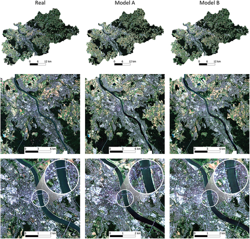
This chapter will describe the results of the synthetic images obtained using the methodology described above. After a brief visual analysis and an illustrated presentation of the resulting images, we will outline the results of the difference and z-transformed difference calculations and subsequently focus on the model’s ability to mimic spectral signatures by breaking down the SID by underlying LULC classes and show exemplary signatures of selected pixels. In the last part of the chapter, we present the results of the FID analysis. Based on a visual evaluation of the resulting synthetic images, the CGAN combined with the patch fusion approach generates artifact-free images on both training data sets. The large-scale synthetic images do not exhibit any seams or irregularities that indicate the edges of individual patches. With a decreasing scale, it becomes evident that Model B creates more crisp and detailed results than Model A, trained on the data set without crop-type information. However, on a very small scale, even Model B cannot reconstruct the original image’s sharpness and richness of detail. Figure 8 compares the original S2 satellite image with the synthetic images created under the two training data sets.

Figure 8. Comparison of resulting synthetic images and the real image under different spatial scales.

3.1. Difference calculation

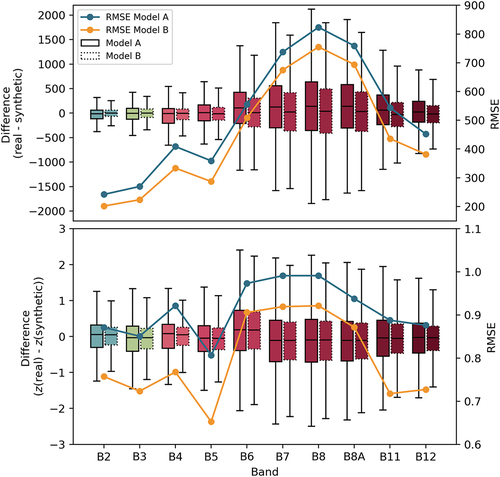
Apart from the visual inspection of the results, several metrics were calculated to measure the image quality compared to the real image. Calculating the difference between the two domains revealed a differentiated curve of errors along the channels under both training data sets, as illustrated in Figure 9. Starting with considerable low RMSE values between 242.1 to 358.9 with Model A and 201.6 to 333.5 under Model B for the bands B2 to B5, the error increased with increasing wavelengths from B6 onwards, reaching the highest uncertainties with RMSE values of 823.5 under Model A and 755.2 under Model B in B8 before decreasing again. Throughout all channels, Model B reaches better error values. A z-transformation preceding the difference calculation, which is intended to remove the influence of brightness deviations to the error, results in a less distinct error distribution along the channels. While band B2 exhibited the lowest error values before the transformation, band B5 showed the lowest RMSE after the transformation, with 0.81 under Model A and 0.65 under Model B. Although the amplitude of the RMSE curve is lower after the transformation, bands B6 to B8A still have the highest errors. Model B remains to provide better RMSEs after the z-transformation throughout all channels.

Figure 9. Difference and z-transformed difference between real and synthetic images.

3.2. Spectral information divergence

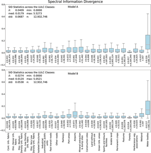
While the difference between the synthetic and the real image’s channels can provide insights into the performance of each individual channel, we utilize the SID to evaluate the model’s capabilities to synthesize the spectral signature for each underlying LULC class, as depicted in Figure 10. Except for wetlands and airports, Model B outperforms Model A in all LULC classes. While Model A has an average SID of 0.041 across all LULC classes, Model B reaches 0.027. Both models reach exceptionally low SIDs for forest areas (mean SID of 0.014 under Model B and 0.017 under Model A) and equally low SIDs for all noncommercial urban classes (0.030–0.04 under Model A and 0.023–0.027 under Model B) in comparison with the average SID value. However, both models suffer from high SIDs in port areas (0.072, 0.052), airports (0.061, 0.073), and water bodies (0.229, 0.217). Based on the variance within the SID scores depending on the underlying LULC classes, we face a class-depending performance difference.

Figure 10. Spectral information divergence boxplots for each LULC class.

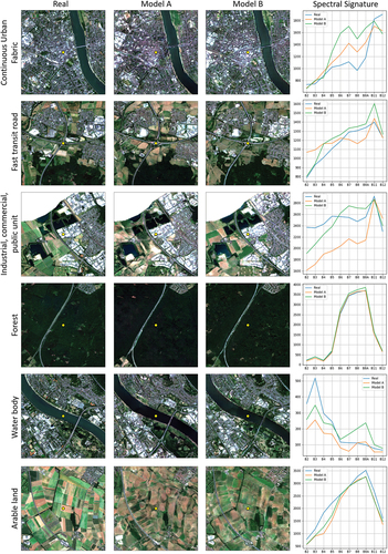
Considering that the SID can provide insights into the similarity between real and synthetic spectral curves between different domains but does not directly depict the spectral signature, we selected some image segments from the large-scale images and plotted the center pixel’s spectral signature of the real and synthetic images. Figure 11 demonstrates that both models mimic the spectral curve’s rough shape. However, signatures of vegetated pixels, e.g. forests or arable land, tend to be closer to the actual curve. Even though the distance between the curves increases within the near-infrared channels for a continuous urban fabric pixel, the curves’ shapes still tend to mimic the local minimums and maximums of the actual signature but shifted in reflectance intensity. In contrast, the models exhibit deficits within the shorter wavelengths over industrial buildings and fail to synthesize the relative constant reflectances between B2 and B8A.

Figure 11. Spectral signatures of exemplary pixels.

3.3. Fréchet inception distance

To prevent subjectivity in the optical evaluation described at the beginning of this section, we calculated the FID and present its results in Table 3. According to the FID, the two models only exhibit minor differences regarding the degree of realism. Analog to the previous z-transformed difference calculation, B8 again stands out with the highest FIDs (Model A: 153.4, Model B: 156.1) and, thus, the poorest performance across all tested channels and channel combinations. Conversely, B2 and B5, which achieved decent results in the previous observations, also achieve low and, therefore, good FID values. Unlike B11 and B12, which exhibit similar good FIDs (<100), B3 and B4 are recognized as being less realistic according to the FID. Besides the individual bands, we also calculated the FID for an RGB and a near-infrared, red and green (NIRRG) band combination. While Model B reached a better FID (117.7) for the RGB combination, Model A performed better on the NIRRG combination with an FID of 118.6 compared to 128.0.

Table 3. FID for different channels and channel combinations. Better performance is highlighted in bold.

Channels	FID Model A	FID Model B
B2	96.5	80.2
B3	117.5	110.4
B4	120.7	114.5
B5	90.9	85.3
B6	104.2	103.5
B7	111.2	110.9
B8	153.4	156.1
B8A	110.5	111.6
B11	98.7	99.4
B12	97.8	90.8
RGB	127.7	117.7
NIRRG	118.6	128.0

According to the similar FID values between the different channel combinations, true- and false-color representations also achieve an equally realistic visual impression.

4. Discussion

During the evaluation of the models’ per-band performance, we discovered that the models have difficulties synthesizing some of the red edge and near-infrared channels, especially B8. Even though those channels predominantly differ in their native resolution, a connection between poor performance and a courser resolution cannot be drawn, as B5, B11, and B12, which also have a resolution of 20 meters, showed promising results.

In line with the results of Abady et al. (2020), the observation of individual spectral signatures indicates certain capabilities of GANs to mimic spectral signatures. However, by using LULC information as conditional inputs to the generator, we are also able to detect and evaluate performance differences for distinct Urban Atlas LULC classes. The SID analysis reveals that besides the band-dependent performance differences, we also face performance differences depending on underlying LULC classes and, thus, on the conditions we feed into the generator. The share of LULC classes is neither balanced within the train nor the test data set. Although this circumstance is inherent in the natural land cover, it manifests itself in poor image textures and unrealistic spectral signatures in under-represented LULC categories, which could be reduced with more balanced training data sets. Even though the Urban Atlas has a high spatial resolution compared to other LULC data sets, some classes, such as airports or forests, exhibit a high degree of generalization. Those areas are represented as a single class, even if several subclasses exist, such as runways and green areas between runways. This insufficient differentiation led to poor results for airport areas. Similarly, the deficits for water bodies can presumably be linked to a lack of differentiation between watercourses, natural lakes, and quarry ponds. While the results indicate that more detailed information about a LULC class (as shown between Model A and B using additional crop type information) eventuates in better model performance for the respective class, there is a need to investigate additional input variables for all classes. However, this study did not cover all existing Urban Atlas classes within the research area, which are thus missing in the evaluation of the model. Even though placeholders instead of no-data values were used for those classes, we did not observe any irregularities in adjacent classes. A training data set that utilizes more regions of the Urban Atlas would close this gap but simultaneously entails quantities of data that are difficult to handle for the hardware used in this study. As the GAN’s inputs are mainly delineated from remote sensing data and thus suffer from uncertainties, a certain amount of error is propagated into the neural network. Taking the Urban Atlas LULC data as an example, the authors report a minimum overall accuracy of 80% for all classes (European Commission 2020). Despite precise pre-processing of the training data during rasterization and transformation in ArcGIS Pro, the individual LULC layers exhibit deficits in their spatial co-registration. This discrepancy between the input data sets, especially between the Urban Atlas LULC and the crop-type data, can be attributed to aleatoric or epistemic uncertainties. Such data uncertainties have also been investigated by W. He et al. (2022), W. He and Jiang (2023) and Elmes et al. (2020). Our method is in line with the procedure recommended by W. He and Jiang (2023) for using CGANs to quantify such uncertainties.

Considering that the FID was initially developed for RGB images, the results of this analysis must be interpreted with caution. Furthermore, the lack of a fixed scale hinders an unambiguous categorization of the results. In order to apply the FID reliably to synthetic multispectral satellite images, the underlying model must be retrained on multispectral images.

During the conceptualization of this study and initial test runs, we used three input bands to generate the 10-channel satellite image. Thereby, we detected numerous artifacts in the synthetic images. We observed a considerable decrease in these artifacts by providing additional input bands, such as a binary band for each Urban Atlas LULC class. The finding that splitting categorical data into several channels can lead to a reduction in artifacts is consistent with the findings of A. N. Wu and Biljecki (2022). Furthermore, the necessity of a band with information about the native size of the patch became apparent during the inference of the model, as the approach used in our study to fuse the patches requires different-sized patches. Applying this approach without encoding the native size of the patch led to substantial irregularities.

Previous studies on synthetic satellite images discussed their role in the initiated debate on Deep Fake Geography in terms of their detection (Zhao et al. 2021) or did not discuss their use in a broader sense (Abady et al. 2020). Even though there is a certain risk of misuse inherent in synthesizing satellite data, the results show the CGAN’s capabilities to reconstruct multispectral images from LULC data. They can, therefore, serve as a useful element in LULC-based application domains, not just as a tool for creating false data in the world of Deep Fake Geography.

5. Conclusion

In this paper, we created a workflow to generate a seamless, large-scale, synthetic multispectral satellite image of the administrative region of Bonn and Rhein-Sieg in North Rhine-Westphalia, Germany. The workflow includes the generation of training data, data normalization with Yeo – Johnson transformation and min-max normalization, CGAN training, the blending of predicted patches to a large-scale image, and its evaluation with several metrics. Even though three of the Urban Atlas classes have not been evaluated due to their absence in the testing area, we conclude that [i] open-source LULC data can provide enough information to a CGAN to generate distinct synthetic features matching with features typical for its LULC category. The provision of additional LULC information, such as crop types, significantly improves the synthetic image regarding its spectral signature and visual perception. Therefore, we conclude [ii] that a CGAN can also synthesize multispectral signatures based on LULC information, although the reliability is strongly dependent on the manifoldness and the categorical and spatial resolution of the provided input data. Regarding the model’s performance on different LULC classes [iii], we deduce that the amount of training pixels per LULC class and the degree of subsummation have a strong influence on the visual realism and the spectral accuracy. Performance differences along the synthetic image’s channels [iv] are apparent but are of ambiguous origin. While this research investigated a U-NET architecture for the generator and a Patch GAN as a discriminator, several alternative architectures are available and might provide better results. However, as pre-trained models for this task are nonexistent, we were not able to compare the results to other publications. The generation of multispectral synthetic satellite images with Transformer Neural Networks should be tested in future studies. As we used a small percentage of the available Urban Atlas in Europe for training, there is still a vast potential to improve the model’s performance through larger training data sets. This study used S2 images captured during the summer months. However, through the implementation of a one-to-many translation, it might be possible to generate synthetic images for each season. The fact that most metrics for the evaluation of synthetic multispectral images are dimensionless, but an exact quantification and classification of the results is necessary emphasizes the need for metrics with fixed scales. We argue that synthetic satellite images can enrich LULC forecasting models and can support scenario-oriented urban planning. However, it must be noted that synthesized satellite images can be misused for disinformation campaigns and thus require well-trained models to expose manipulated or synthetic images.

6. Supplements

6.1. Software

Table 4. Relevant Software and Python packages used in different stages of the research.

Stage	Software/Language	Packages
Data Preparation	ArcGIS Pro
	QGIS
	Google Earth Engine
	Python	numpy, tifffile, scikit-learn, pandas, joblib, patchify, rasterio, random
Training & Inference	Python	torch, torchvision, albumentations, numpy, tifffile,natsort, tqdm, rasterio, csv, sympy, math, pandas
Evaluation & Figure Design	ArcGIS Pro
	GIMP
	Python	numpy, tifffile, matplotlib, pandas, torch, torchmetrics, patchify, numpy, csv

Acknowledgments

We acknowledge support by the DFG Open Access Publication Funds of the Ruhr-Universität Bochum. This study was conducted at and with the infrastructure provided by the Institute of Geography, Ruhr University Bochum, Germany. We want to thank Prof. Dr. Carsten Jürgens and Stefanie Steinbach for their valuable feedback as we finalized the manuscript and Jan-Philipp Langenkamp for the competent professional discussions.

Disclosure statement

No potential conflict of interest was reported by the author(s).

Data availability statement

Data available on request from the authors.

Additional information

Funding

No additional funding was received.

References

- Abady, L., M. Barni, A. Garzelli, and B. Tondi. 2020. “GAN Generation of Synthetic Multispectral Satellite Images.” Image and Signal Processing for Remote Sensing XXVI, edited by C. Notarnicola, F. Bovenga, L. Bruzzone, F. Bovolo, J. A. Benediktsson, E. Santi, and N. Pierdicca. 19. SPIE. https://www.spiedigitallibrary.org/conference-proceedings-of-spie/11533/2575765/GAN-generation-of-synthetic-multispectral-satellite-images/10.1117/12.2575765.full.
- Abady, L., J. Horváth, B. Tondi, E. J. Delp, and M. Barni. 2022. “Manipulation and Generation of Synthetic Satellite Images Using Deep Learning Models.” Journal of Applied Remote Sensing 16 (4). https://doi.org/10.1117/1.JRS.16.046504.
- Adegun, A., S. Viriri, and J. Tapamo. 2023. “Review of Deep Learning Methods for Remote Sensing Satellite Images Classification: Experimental Survey and Comparative Analysis.” Journal of Big Data 10 (1). https://doi.org/10.1186/s40537-023-00772-x.
- Benjdira, B., Y. Bazi, A. Koubaa, and K. Ouni. 2019. “Unsupervised Domain Adaptation Using Generative Adversarial Networks for Semantic Segmentation of Aerial Images.” Remote Sensing 11 (11): 1369. https://doi.org/10.3390/rs11111369.
- Borji, A. 2022. “Pros and Cons of GAN Evaluation Measures: New Developments.” Computer Vision and Image Understanding 215:103329. https://doi.org/10.1016/j.cviu.2021.103329.
- Cai, G., H. Ren, L. Yang, N. Zhang, M. Du, and C. Wu. 2019. “Detailed Urban Land Use Land Cover Classification at the Metropolitan Scale Using a Three-Layer Classification Scheme.” Sensors (Basel, Switzerland) 19 (14): 14. https://doi.org/10.3390/s19143120.
- Campos-Taberner, M., F. Javier García-Haro, B. Martínez, E. Izquierdo-Verdiguier, C. Atzberger, G. Camps-Valls, and M. Amparo Gilabert. 2020. “Understanding Deep Learning in Land Use Classification Based on Sentinel-2 Time Series.” Scientific Reports 10 (1): 17188. https://doi.org/10.1038/s41598-020-74215-5.
- Chang, C.-I. 1999. “Spectral Information Divergence for Hyperspectral Image Analysis.” IEEE 1999 International Geoscience and Remote Sensing Symposium. IGARSS’99 (Cat. No. 99CH36293), 509–11. IEEE.
- Chang, C.-I. 2000. “An Information-Theoretic Approach to Spectral Variability, Similarity, and Discrimination for Hyperspectral Image Analysis.” IEEE Transactions on Information Theory 46 (5): 1927–20. https://doi.org/10.1109/18.857802.
- Couclelis, H. 1986. “Artificial Intelligence in Geography: Conjectures on the Shape of Things to Come.” The Professional Geographer 38 (1): 1–11. https://doi.org/10.1111/j.0033-0124.1986.00001.x.
- Elmes, A., H. Alemohammad, R. Avery, J. E. Kelly Caylor, L. Fishgold, M. Friedl, M. Friedl, et al. 2020. “Accounting for Training Data Error in Machine Learning Applied to Earth Observations.” Remote Sensing 12 (6): 1034. https://doi.org/10.3390/rs12061034.
- ESRI. 2020. “Deep Learning Libraries Installers for ArcGIS.” Accessed January 30, 2024. Unpublished manuscript. https://github.com/Esri/deep-learning-frameworks.
- European Commission. 2020. Mapping Guide V6.3 for a European Urban Atlas. Accessed 25 October. https://land.copernicus.eu/en/technical-library/urban_atlas_2012_2018_mapping_guide/@@download/file.
- European Environment Agency. 2020. “Urban Atlas Land Cover/Land Use 2018 (Vector).” Europe. Jul, 6–Yearly.
- Foster, D. 2020. Generatives Deep Learning: Maschinen Das Malen, Schreiben Und Komponieren Beibringen. 1. Auflage. Heidelberg: O’Reilly.
- Gong, Y., F. Zhang, X. Jia, Z. Mao, X. Huang, and D. Li. 2022. “Instance Segmentation in Very High Resolution Remote Sensing Imagery Based on Hard-To-Segment Instance Learning and Boundary Shape Analysis.” Remote Sensing 14 (1): 23. https://doi.org/10.3390/rs14010023.
- Goodfellow, I., J. Pouget-Abadie, M. Mirza, B. Xu, D. Warde-Farley, S. Ozair, A. Courville, and Y. Bengio. 2014. “Generative Adversarial Networks.” stat.ML 1–9. https://doi.org/10.48550/arXiv.1406.2661.
- Gorelick, N., M. Hancher, M. Dixon, S. Ilyushchenko, D. Thau, and R. Moore. 2017. “Google Earth Engine: Planetary-Scale Geospatial Analysis for Everyone.” Remote Sensing of Environment 202:18–27. https://doi.org/10.1016/j.rse.2017.06.031.
- He, W., and Z. Jiang. 2023. “Uncertainty Quantification of Deep Learning for Spatiotemporal Data: Challenges and Opportunities.” cs.LG 1–5. https://doi.org/10.48550/arXiv.2311.02485.
- Heusel, M., H. Ramsauer, T. Unterthiner, B. Nessler, and S. Hochreiter. 2017. “GANs Trained by a Two Time-Scale Update Rule Converge to a Local Nash Equilibrium.” https://doi.org/10.48550/arXiv.1706.08500.
- He, C., Y. Zhao, J. Dong, and Y. Xiang. 2022. “Use of GAN to Help Networks to Detect Urban Change Accurately.” Remote Sensing 14 (21): 5448. https://doi.org/10.3390/rs14215448.
- He, W., J. Zhe, K. Marcus, X. Yiqun, J. Xiaowei, Y. Da, and Z. Yang. 2022. “Quantifying and Reducing Registration Uncertainty of Spatial Vector Labels on Earth Imagery.” In Proceedings of the 28th ACM SIGKDD Conference on Knowledge Discovery and Data Mining, edited by A. Zhang and H. Rangwala, 554–564. New York, NY, USA: ACM.
- Hou, B., Q. Liu, H. Wang, and Y. Wang. 2020. “From W-Net to CDGAN: Bi-Temporal Change Detection via Deep Learning Techniques.” IEEE Transactions on Geoscience & Remote Sensing 58 (3): 1790–1802. https://doi.org/10.48550/arXiv.2003.06583.
- Isola, P., J. Zhu, T. Park, and A. Efros. 2017 “Unpaired Image-To-Image Translation Using Cycle-Consistent Adversarial Networks.” In IEEE International Conference on Computer Vision (ICCV), 2242–2251. https://doi.org/10.1109/ICCV.2017.244.
- Isola, P., J.-Y. Zhu, T. Zhou, and A. E. Alexei. 2016. “Image-To-Image Translation with Conditional Adversarial Networks” cs.CV 1–17. https://doi.org/10.48550/arXiv.1611.07004.
- Ji, S., D. Wang, and M. Luo. 2021. “Generative Adversarial Network-Based Full-Space Domain Adaptation for Land Cover Classification from Multiple-Source Remote Sensing Images.” IEEE Transactions on Geoscience & Remote Sensing 59 (5): 3816–3828. https://doi.org/10.1109/TGRS.2020.3020804.
- JRC. 2021. Eurocropmap 2018. Accessed January 16, 2024. Unpublished manuscript. https://publications.jrc.ec.europa.eu/repository/handle/JRC125312.
- Lang, L., K. Xu, Q. Zhang, and D. Wang. 2021. “Fast and Accurate Object Detection in Remote Sensing Images Based on Lightweight Deep Neural Network.” Sensors (Basel, Switzerland) 21 (16): 5460. https://doi.org/10.3390/s21165460.
- Lebedev, M. A., Y. V. Vizilter, O. V. Vygolov, V. A. Knyaz, and A. Y. Rubis. 2018. “Change Detection in Remote Sensing Images Using Conditional Adversarial Networks.” The International Archives of the Photogrammetry, Remote Sensing and Spatial Information Sciences XLII-2:565–571. https://doi.org/10.5194/isprs-archives-XLII-2-565-2018.
- Li, J., Z. Chen, X. Zhao, and L. Shao. 2020. “MapGAN: An Intelligent Generation Model for Network Tile Maps.” Sensors (Basel, Switzerland) 20 (11): 3119. https://doi.org/10.3390/s20113119.
- Liu, B., Z. Li, J. Li, H. Zhao, W. Liu, Y. Li, Y. Wang, H. Chen, and W. Cao. 2021. “Saliency-Guided Remote Sensing Image Super-Resolution.” Remote Sensing 13 (24): 5144. https://doi.org/10.3390/rs13245144.
- Liu, Y., D. Minh Nguyen, N. Deligiannis, W. Ding, and A. Munteanu. 2017. “Hourglass-ShapeNetwork Based Semantic Segmentation for High Resolution Aerial Imagery.” Remote Sensing 9 (6): 522. https://doi.org/10.3390/rs9060522.
- Li, Z., Y. Wang, N. Zhang, Y. Zhang, Z. Zhao, D. Xu, G. Ben, and Y. Gao. 2022. “Deep Learning-Based Object Detection Techniques for Remote Sensing Images: A Survey.” Remote Sensing 14 (10): 2385. https://doi.org/10.3390/rs14102385.
- Lu, H., Q. Liu, X. Liu, and Y. Zhang. 2021. “A Survey of Semantic Construction and Application of Satellite Remote Sensing Images and Data.” Journal of Organizational and End User Computing 33 (6): 1–20. https://doi.org/10.4018/JOEUC.20211101.oa29.
- Lv, J., Q. Shen, M. Lv, Y. Li, L. Shi, and P. Zhang. 2023. “Deep Learning-Based Semantic Segmentation of Remote Sensing Images: A Review.” Frontiers in Ecology and Evolution: 11. https://doi.org/10.3389/fevo.2023.1201125.
- Mandal, V., A. Rashid Mussah, P. Jin, and Y. Adu-Gyamfi. 2020. “Artificial Intelligence-Enabled Traffic Monitoring System.” Sustainability 12 (21): 9177. https://doi.org/10.3390/su12219177.
- Mateo-García, G., V. Laparra, C. Requena-Mesa, and L. Gómez-Chova. 2021. “Generative Adversarial Networks in the Geosciences.” In Deep Learning for the Earth Sciences: A Comprehensive Approach to Remote Sensing, Climate Science, and Geosciences, edited by G. Camps-Valls, D. Tuia, X. X. Zhu, and M. Reichstein, 24–36. S.l: JOHN WILEY.
- Mirza, M., and S. Osindero. 2014. “Conditional Generative Adversarial Nets.” cs.LG 1–7. https://doi.org/10.48550/arXiv.1411.1784.
- Persson, A. 2021. GitHub Repository - Aladdin Persson.” Unpublished manuscript, last modified December 19, 2023. https://github.com/aladdinpersson.
- Qiu, C., L. Mou, M. Schmitt, and X. X. Zhu. 2019. “Local Climate Zone-Based Urban Land Cover Classification from Multi-Seasonal Sentinel-2 Images with a Recurrent Residual Network.” ISPRS Journal of Photogrammetry and Remote Sensing: Official Publication of the International Society for Photogrammetry and Remote Sensing (ISPRS) 154:151–162. https://doi.org/10.1016/j.isprsjprs.2019.05.004.
- Qiu, C., X. Tong, M. Schmitt, B. Bechtel, and X. X. Zhu. 2020. “Multilevel Feature Fusion-Based CNN for Local Climate Zone Classification from Sentinel-2 Images: Benchmark Results on the So2Sat LCZ42 Dataset.” IEEE Journal of Selected Topics in Applied Earth Observations & Remote Sensing 13:2793–2806. https://doi.org/10.1109/JSTARS.2020.2995711.
- Rosentreter, J., R. Hagensieker, and B. Waske. 2020. “Towards Large-Scale Mapping of Local Climate Zones Using Multitemporal Sentinel 2 Data and Convolutional Neural Networks.” Remote Sensing of Environment 237:111472. https://doi.org/10.1016/j.rse.2019.111472.
- Schmitt, M., L. Haydn Hughes, C. Qiu, and X. Xiang Zhu. 2019. “SEN12MS: A Curated Dataset of Georeferenced Multi-Spectral Sentinel-1/2 Imagery for Deep Learning and Data Fusion.” http://arxiv.org/pdf/1906.07789.pdf.
- Siracusa, G., D. Seychell, and M. Bugeja. 2021. “Blending Output from Generative Adversarial Networks to Texture High-Resolution 2D Town Maps for Roleplaying Games.” In 2021 IEEE Conference on Games (CoG), University of Copenhagen (virtual), 1–8. IEEE.
- Soto, P. J., G. A. O. P. Costa, R. Q. Feitosa, P. N. Happ, M. X. Ortega, J. Noa, C. A. Almeida, and C. Heipke. 2020. “Domain Adaptation with CYCLEGAN for Change Detection in the Amazon Forest.” International Archives of the Photogrammetry, Remote Sensing and Spatial Information Sciences XLIII-B3-2020:1635–1643. https://doi.org/10.5194/isprs-archives-XLIII-B3-2020-1635-2020.
- Szegedy, C., V. Vanhoucke, S. Ioffe, J. Shlens, and Z. Wojna. 2015. “Rethinking the Inception Architecture for Computer Vision” cs.CV 1–10. https://doi.org/10.48550/arXiv.1512.00567.
- Wang, D., C.-T. Lu, and Y. Fu. 2022. “Towards Automated Urban Planning: When Generative and ChatGPT-Like AI Meets Urban Planning.” ACM Transactions on Spatial Algorithms and Systems 1 (1): 1–19. https://doi.org/10.48550/arXiv.2304.03892.
- Wu, A. N., and F. Biljecki. 2022. “GANmapper: Geographical Data Translation.” International Journal of Geographical Information Science 36 (7): 1394–1422. https://doi.org/10.1080/13658816.2022.2041643.
- Wurm, M., A. Droin, T. Stark, C. Geiß, W. Sulzer, and H. Taubenböck. 2021. “Deep Learning-Based Generation of Building Stock Data from Remote Sensing for Urban Heat Demand Modeling.” IJGI 10 (1): 23. https://doi.org/10.3390/ijgi10010023.
- Yang, F., X. Yuan, J. Ran, W. Shu, Y. Zhao, A. Qin, and C. Gao. 2021. “Accurate Instance Segmentation for Remote Sensing Images via Adaptive and Dynamic Feature Learning.” Remote Sensing 13 (23): 4774. https://doi.org/10.3390/rs13234774.
- Zhang, Y., Y. Yin, R. Zimmermann, G. Wang, J. Varadarajan, and S. Ng. 2020. “An Enhanced GAN Model for Automatic Satellite-To-Map Image Conversion.” IEEE Access 8:176704–176716. https://doi.org/10.1109/ACCESS.2020.3025008.
- Zhao, B., S. Zhang, C. Xu, Y. Sun, and C. Deng. 2021. “Deep Fake Geography? When Geospatial Data Encounter Artificial Intelligence.” Cartography and Geographic Information Science 48 (4): 338–352. https://doi.org/10.1080/15230406.2021.1910075.
- Zhu, F., C. Wang, B. Zhu, C. Sun, and C. Qi. 2023. “An Improved Generative Adversarial Networks for Remote Sensing Image Super-Resolution Reconstruction via Multi-Scale Residual Block.” The Egyptian Journal of Remote Sensing and Space Science 26 (1): 151–160. https://doi.org/10.1016/j.ejrs.2022.12.008.