
 ?Mathematical formulae have been encoded as MathML and are displayed in this HTML version using MathJax in order to improve their display. Uncheck the box to turn MathJax off. This feature requires Javascript. Click on a formula to zoom.
ABSTRACT
Time series analysis of medium-resolution multispectral satellite imagery is critical to investigate forest disturbance dynamics at the landscape scale. In particular, the spatial, temporal, and radiometric consistency of Landsat time series data provides unprecedented insight into past disturbances that occurred over the last four decades. Several Landsat time series-based algorithms have been developed to automate the detection of forest disturbances. However, automated detection of non-stand-replacing disturbances based on Landsat time series remains a challenging task due to the difficulty of effectively separating them from spectral noise. Here, we present the High-dimensional detection of Landscape Dynamics (HILANDYN) algorithm, which exploits spatial and spectral information provided by Landsat time series to detect forest disturbance dynamics retrospectively. A novel and unsupervised procedure for changepoint detection in high-dimensional time series allows HILANDYN to perform the temporal segmentation of inter-annual time series into linear trends. The algorithm embeds a noise filter to remove spurious changepoints caused by residual spectral noise in the time series. We tested HILANDYN to detect disturbances that occurred in the forests of the European Alps over a period of 39 years, i.e. between 1984 and 2022, and evaluated its accuracy using a validation dataset of 3000 plots randomly located inside and outside the disturbed patches. We compared HILANDYN with the Bayesian Estimator of Abrupt change, Seasonality, and Trend (BEAST), which is a well-established and high-performing time series-based algorithm for changepoint detection. The quantitative results highlighted that the number of bands, i.e. original Landsat bands and spectral indices, included in the high-dimensional time series and the threshold controlling the significance of changepoints strongly influenced the user’s accuracy (UA). Conversely, changes in the combinations of bands primarily affected the producer’s accuracy (PA). HILANDYN achieved an F1 score of 0.801, which increased to 0.833 when we activated the noise filter, allowing the algorithm to balance UA (83.1%) and PA (83.5%). The qualitative results showed that disturbed forest patches detected by HILANDYN were characterized by a high spatio-temporal consistency, regardless of the disturbance severity. Furthermore, our algorithm was able to detect forest patches associated with secondary disturbances, such as salvage logging, that occur in close succession with respect to the primary event. The comparison with BEAST evidenced a similar sensitivity of the algorithms to non-stand-replacing events, as both achieved comparable PA. However, BEAST struggled to balance UA and PA when using a single parameter set, achieving a maximum F1 score of 0.717. Moreover, the computational efficiency of BEAST in processing high-dimensional time series was very limited due to its univariate nature based on the Bayesian approach. The adaptability of HILANDYN to detect a wide range of disturbance severities using a single parameter set and its computational efficiency in handling high-dimensional time series promotes its scalability to large study areas characterized by heterogeneous ecological conditions.
1. Introduction
Disturbances such as wildfires, windthrows, and insect or pathogen outbreaks are key components of forest ecosystems (Turner Citation2010). They alter the state and trajectories of ecosystems and generate heterogeneity in space and time. The intensification of climate-driven changes in disturbance regimes has been observed globally, with negative impacts on the structure, functions, and composition of forests (Forzieri et al. Citation2021; Seidl et al. Citation2017). Shifts in disturbance patterns toward more frequent, larger and more severe events can drastically impair the resilience of forests and trigger transitions to a non-forest state (Johnstone et al. Citation2016; Seidl et al. Citation2016). Besides stand-replacing disturbances, long-term studies based either on field (Andrus et al. Citation2021; Camarero et al. Citation2015) or remote sensing data (Cohen et al. Citation2016; Senf et al. Citation2018) highlighted increasing trends in tree mortality rates, associated with gradual, non-stand-replacing disturbances. Warming temperatures and increases in severe and prolonged droughts driven by climate change resulted in extensive forest decline globally (Allen, Breshears, and McDowell Citation2010, Citation2015). Apart from the direct effects of climate change, modifications of the interactions between disturbance agents (Seidl et al. Citation2017) and land-use change patterns, such as land abandonment (Mantero et al. Citation2020), further drove shifts in disturbance regimes. Identifying changes in disturbance regimes that occurred over the last decades has crucial implications for current and future management policies (Leverkus et al. Citation2021).
Satellite-based remote sensing is a fundamental data source for forest ecologists as it enables a comprehensive understanding of ecological processes both in the spatial and temporal dimensions (Kennedy et al. Citation2014; Senf Citation2022). In particular, continuously acquired data by Landsat satellites over the last four decades provide a unique opportunity to reconstruct long-term forest disturbance dynamics at the landscape scale (Senf Citation2022; Wulder et al. Citation2019). The opening of the U.S. Geological Survey (USGS) Landsat archive in 2008 prompted a rapid increase in the use of time series for analyzing forest ecosystem dynamics from regional to global scales (Banskota et al. Citation2014; Wulder et al. Citation2012).
Several Landsat time series-based change detection algorithms have been developed so far, either to explicitly map forest dynamics or target a broader range of land cover changes (Zhu Citation2017). Some of these algorithms, such as LandTrendr (Landsat-based Detection of Trends in Disturbance and Recovery; Kennedy, Yang, and Cohen Citation2010) and CCDC (Continuous Change Detection and Classification; Zhu and Woodcock Citation2014), gained considerable popularity, thanks also to their implementation in the Google Earth Engine platform (Pasquarella et al. Citation2022). Both LandTrendr and CCDC perform a temporal segmentation, i.e. they partition time series into discrete intervals based on the similarity between consecutive observations, at the pixel level (Pasquarella et al. Citation2022). Whilst, based on a similar theoretical framework, these algorithms present fundamental differences in the characteristics of the input time series and the mathematical approaches they rely on. LandTrendr is an offline algorithm, i.e. it operates on completely available time series, that segments inter-annual data into linear trends. Conversely, CCDC is an online algorithm, i.e. it processes continuously acquired data, that fits harmonic functions for modeling intra-annual phenological cycles. LandTrendr is univariate as it can segment one band, i.e. original reflectance bands and spectral indices, sensu Cohen et al. (Citation2020), at each run, while CCDC is multivariate as it simultaneously analyzes multiple bands (Zhu Citation2017). C2C (Composite2Change; Hermosilla et al. Citation2015) and VeRDET (Vegetation Regeneration and Disturbance Estimates through Time; Hughes, Kaylor, and Hayes Citation2017) are among the algorithms that share characteristics with LandTrendr, as they are offline, univariate, and segment inter-annual time series into linear trends. On the contrary, EWMACD (Exponentially Weighted Moving Average Change Detection; Brooks et al. Citation2014) and COLD (COntinuous monitoring of Land Disturbance; Zhu et al. Citation2019) are similar to CCDC, as they model phenological cycles using continuously acquired data.
The sensitivity of Landsat time series-based algorithms to non-stand-replacing disturbances, i.e. those causing partial canopy loss, has been reported to be somewhat limited compared, for example, to visual interpretation of spectral-temporal profiles (Cohen et al. Citation2017) or bi-temporal burn severity indices (Rodman et al. Citation2021). Indeed, extracting the weak signals associated with non-stand-replacing disturbances is hindered by noise in Landsat time series, which is generated by uncertainties in pre-processing operations like georeferencing and atmospheric correction (Cohen et al. Citation2017; Rodman et al. Citation2021; Vogelmann et al. Citation2016). A key issue when targeting non-stand-replacing disturbances is the proper optimization of the parameters of an algorithm in order to balance omission and commission errors (Cohen et al. Citation2017; Ye et al. Citation2021).
Various ensemble approaches have been proposed in the context of Landsat time series-based algorithms as they improved the accuracy of disturbance maps, primarily by increasing the sensitivity to low-severity events (Cohen et al. Citation2018; Healey et al. Citation2018; Schultz et al. Citation2016). Algorithm ensembles are built by aggregating results from multiple change detection algorithms that are executed in parallel (Cohen et al. Citation2020; Healey et al. Citation2018; Hislop et al. Citation2019). Conversely, multispectral ensembles (Cohen et al. Citation2018; Marzo et al. Citation2021; Schultz et al. Citation2016) involve the analysis of several bands through parallel runs of a univariate algorithm, which outputs are then dissolved into a single result using a supervised classifier, e.g. random forest. Considering individual algorithms, BEAST (Bayesian Estimator of Abrupt change, Seasonality, and Trend; Zhao et al. Citation2019) employs an ensemble learning technique termed Bayesian model averaging (BMA). BMA involves combining the estimates of many candidate models by quantifying their usefulness according to a Bayesian posterior probability. This approach allows BEAST to explicitly quantify model uncertainty and deal with complex nonlinear signals in the seasonal and trend components. BEAST exhibited solid performance in detecting both stand-replacing and non-stand-replacing disturbances using time series of medium-resolution satellite data, such as Landsat (Hu et al. Citation2021; Moreno-Fernández et al. Citation2021) and Sentinel-2 (Giannetti et al. Citation2021; Mulverhill, Coops, and Achim Citation2023).
Spectral information from the spatial context has been integrated into Landsat time series-based algorithms, either before or after temporal segmentation (Hermosilla et al. Citation2015; Hughes, Kaylor, and Hayes Citation2017; Meng et al. Citation2021). Moving window-based approaches have been employed before temporal segmentation to increase the accuracy of forest disturbance (Hamunyela, Verbesselt, and Herold Citation2016) and recovery (Meng et al. Citation2021) maps. Object-based image analysis (OBIA) is another effective approach for analyzing change processes in forest landscapes at different spatial scales (Gómez, White, and Wulder Citation2011). In this sense, the VeRDET algorithm (Hughes, Kaylor, and Hayes Citation2017) spatially segments individual bands into patches of constant values to reduce the heterogeneity within the same land cover class prior to perform temporal segmentation. Applying spatial context approaches after temporal segmentation is also effective for enhancing forest disturbance maps. The C2C algorithm (Hermosilla et al. Citation2015), for example, performs postprocessing operations based on moving windows to improve the spatial-temporal consistency of disturbance patches. In a similar fashion, spatial filtering operations allowed Senf and Seidl (Citation2020) and Ye et al. (Citation2021) to reduce omission and commission errors associated with small patches in the disturbance maps. Recently, Ye et al., (Citation2023) have integrated OBIA into a COLD-like algorithm for identifying change objects, i.e. regions of homogeneous change in space and time, at different spatial scales.
A marked increase in the availability of statistical methods for changepoint detection in multivariate and high-dimensional time series, i.e. time series with dimensions of the same order of magnitude of the observations or even larger, has been observed in recent years (Cho et al. Citation2021; Truong, Oudre, and Vayatis Citation2020). To deal with the complexity associated with multivariate time series, one common approach is to aggregate a test statistic (Groen, Kapetanios, and Price Citation2013) or project the time series to a single dimension and then process the data with a univariate method (Wang and Samworth Citation2018). Assumptions on the proportion of time series that undergo a change determine the most appropriate aggregation method (Groen, Kapetanios, and Price Citation2013). For example, the widely used CUSUM statistic for detecting structural changes (Brown, Durbin, and Evans Citation1975) has been aggregated across time series using either the average or the maximum (Groen, Kapetanios, and Price Citation2013; Jirak Citation2015). Generally, the average of a test statistic performs better when a change occurs in the majority of the time series, i.e. a dense change, while the maximum is more appropriate for changes occurring only in a fraction of them, i.e. a sparse change (Groen, Kapetanios, and Price Citation2013; Jirak Citation2015). Changepoint methods have primarily focused on detecting changes in the mean associated with constant signals, though some approaches use piecewise polynomial models to segment time series (Cho et al. Citation2021).
Here, we aimed to develop a Landsat time series-based algorithm for retrospectively mapping forest disturbance and recovery dynamics that overcomes some of the major limitations posed by existing approaches. These include the ability to simultaneously analyze all the dimensions of Landsat data, i.e. spatial, temporal, and spectral, the need for extensive parametrization tuning, and the balancing of omission and commission errors while targeting non-stand-replacing events. The algorithm, named High-dimensional detection of Landscape Dynamics (HILANDYN), harnesses an offline and unsupervised temporal segmentation procedure for detecting changes in linear trends derived from high-dimensional time series containing multispectral and spatial context information. Though HILANDYN can detect changes associated with forest disturbances and recovery processes, here, we focused only on disturbance detection. In particular, we aimed to (i) assess the sensitivity of HILANDYN to stand-replacing and non-stand-replacing disturbances both quantitatively and qualitatively, and (ii) to compare the proposed approach with the BEAST algorithm.
The remainder of the article is organized as follows. In Section 2, we provide details on the study area and a technical description of the algorithm. In Section 3, we present quantitative and qualitative results on forest disturbance detection obtained with HILANDYN, including the comparison with a recent time series-based algorithm. In Section 4, we discuss the strengths and weaknesses of the proposed algorithm and how it compares to state-of-the-art change detection algorithms.
2. Materials and methods
2.1. Study area
Our study area encompasses the core mountainous area of the European Alps as defined by the Alpine Convention (Plangger Citation2020); its area is 190,706 km2, of which 51% is covered by forests according to the Copernicus Dominant Leaf Type 2018 map (European Environmental Agency Citation2020; ). Elevation ranges between 0 and 4807 m a.s.l. (Mont Blanc), with an average altitude of 1293 m a.s.l. According to the official European biogeographical regions (European Environment Agency Citation2016), the study area includes Alpine, Continental, and Mediterranean regions. Climate ranges from oceanic to dry, with mean temperatures ranging from less than 0° to 10° (Nigrelli and Chiarle Citation2023) and annual precipitation from 400 to 3000 mm (Isotta et al. Citation2014). Forests dominated by broadleaved species occupy 45,088 km2, while those dominated by conifers amount to 52,694 km2, according to the Dominant Leaf Type 2018 map (European Environmental Agency Citation2020). Oaks (Quercus spp.) dominate the forests at lower elevations, while silver fir (Abies alba Mill.), beech (Fagus sylvatica L.), and Scots pine (Pinus sylvestris L.) dominate in the montane belt. The most common species in the subalpine belt are European larch (Larix decidua Mill.), Norway spruce (Picea abies (L.) H. Karst.), and Swiss stone pine (Pinus cembra L.).
Figure 1. Geographic location of the study area and validation plots with information from the Dominant Leaf Type 2018 forest cover layer (European Environmental Agency Citation2020) and Landsat Path/Row coverage (World Reference System 2). The base layer corresponds to the hill shade derived from the 25 m EU-DEM digital surface model.
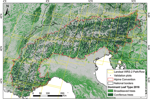
Natural disturbances in the European Alps mainly include windthrows, wildfires, insect outbreaks, and snow avalanches (Bebi et al. Citation2017). Windthrows are by far the most important disturbances in terms of size and severity (Kulakowski et al. Citation2016) and are usually associated with winter storms. Wildfires, which occur primarily in the southern and central Alps, are largely driven by the land abandonment of rural areas, which has led to fuel accumulation and increased connectivity (Bebi et al. Citation2017). Bark beetle outbreaks are the most important biotic disturbances in the European Alps and typically occur shortly after a windthrow. A strong increasing trend in damage to timber volume caused by bark beetles has been observed in the Alps over the last decades due to favorable climatic conditions, such as warming temperatures and prolonged drought periods (Patacca et al. Citation2023).
2.2. Landsat data
Our Landsat dataset included Collection 2 imagery acquired in 30 scenes () between 1984 and 2022 by the Thematic Mapper (TM), Enhanced Thematic Mapper + (ETM+), and Operational Land Imager (OLI) sensors. We retrieved all Level 2 Tier 1 imagery with <80% cloud cover acquired between May and October from the U.S. Geological Survey EarthExplorer tool. We removed pixels contaminated by clouds, cloud shadows, and snow using the Quality Assessment (QA) band bundled with each Landsat image and produced through the C Function of Mask (CFmask) algorithm (Foga et al. Citation2017).
We created a total of 39 pixel-based annual reflectance composites using the weighted geometric median (Morresi et al. Citation2022; Roberts, Wilford, and Ghattas Citation2019) based on the six reflectance bands (Blue, Green, Red, NIR, SWIR1, and SWIR2) of the TM/ETM+ sensors and the corresponding OLI bands relative to the growing season, i.e. from June 1 to September 30. Following Morresi et al. (Citation2022), the compositing time window iteratively widened up to 20 days on both of its sides until at least three clear observations were found in order to minimize data gaps. To reduce the presence of artifacts generated by residual clouds and cloud shadows in reflectance composites, we computed pixel-wise weights relative to the NDVI value () and the Euclidean distance to clouds and cloud shadows (
) for each valid observation within the compositing time window. In particular, the compositing algorithm prioritized observations with a high NDVI, as these were typically not contaminated by clouds or cloud shadows (Qiu et al. Citation2023). Furthermore,
increased the importance of those observations acquired close to the peak of the growing season, when NDVI typically reaches its maximum. The inclusion of
in the compositing algorithm limited the influence of undetected cloud shadows, which can exhibit high NDVI values due to low reflectance of both the Red and NIR. To compute
, we used the sigmoid function proposed by Frantz et al. (Citation2017), which can assume values in the interval [0, 1] depending on the requested distance (
) parameter. We set
equal to 1500 m, i.e. 50 Landsat pixels, as proposed by White et al. (Citation2014).
We tested HILANDYN using the six Landsat bands included in the annual reflectance composites and eight spectral indices ().
Table 1. List of the spectral indices used in this study.
2.3. Overview of the algorithm
HILANDYN aims to map forest patches characterized by disturbance and recovery dynamics through a changepoint analysis based on linear trends derived from high-dimensional Landsat time series. Specifically, a procedure called High-dimensional Trend Segmentation (HiTS, Maeng Citation2019, publicly available at https://github.com/hmaeng/HiTS) is at the core of our algorithm. The HiTS procedure is a generalization to higher dimensions of the TrendSegment procedure (Maeng and Fryzlewicz Citation2023), which was developed to detect multiple changepoints in linear trends for univariate data sequences.
HILANDYN builds high-dimensional time series by extracting data from time-ordered sequences of raster cubes using a three-dimensional spatial kernel (). The number of variables in the high-dimensional time series corresponds to the product between the number of pixels in the spatial kernel and the number of bands. Here, we employed a three-by-three kernel, i.e. nine connected Landsat pixels. Our preliminary tests showed that this kernel dimension was adequate to provide spatial context information when detecting forest dynamics with Landsat data. Other studies (Hermosilla et al. Citation2015; Meng et al. Citation2021) used the same kernel dimension with Landsat time series-based change detection algorithms. Although not specified in the HiTS procedure, we recommend that high-dimensional time series contain at least six valid observations for the algorithm to work properly.
Figure 2. Flowchart of the main operations performed by HILANDYN. Input data consist of four-dimensional raster cubes where bands and time form the third and fourth dimensions, respectively. A three-dimensional spatial kernel is employed on a pixel basis to build -dimensional time series with a matrix form of the dimension
. The core operations performed by HILANDYN on
-dimensional time series are described in the orange box.
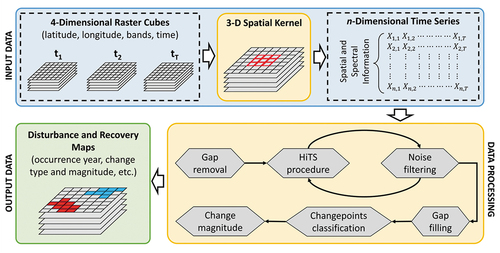
Initially, HILANDYN removes gaps with one-year length from high-dimensional time series while discards those with longer gaps. It then employs an iterative procedure to discern between changepoints associated with forest dynamics and those caused by impulsive noise, i.e. outliers in the spectral signal that are caused, for example, by undetected clouds, cloud shadows, or haze (Hermosilla et al. Citation2015; Kennedy, Yang, and Cohen Citation2010, ). If changepoints and gaps co-occur in a multispectral time series, HILANDYN updates the corresponding year of change depending on the number of gaps preceding each changepoint. It imputes data gaps using values of linear segments previously estimated by the HiTS procedure. Specifically, gaps located at the vertices of segments of at least 3 years in length are imputed using linear extrapolation based on the two preceding values. Otherwise, gaps are filled using the preceding value. Gaps located in the middle of a segment are filled using linear interpolation.
HILANDYN classifies changepoints as disturbances or growth events if at least half of the bands () in the focal pixel follow the pattern of the spectral change associated with that event. In particular, the algorithm evaluates only those bands whose original and estimated values feature the same direction of spectral change. The spectral change magnitude of each event corresponds to the median of the relative change magnitudes among bands, using all the pixels in the spatial kernel. Following Cohen et al. (Citation2016), change magnitudes are relativized using pre-disturbance values.
The implementation of HILANDYN in the C++ language through the Application Programming Interface (API) provided by the Armadillo open-source linear algebra library (Sanderson and Curtin Citation2016) ensured computational efficiency even when the number of variables in high-dimensional time series was high, e.g. more than 100.
2.4. HiTS procedure
The changepoint model proposed in the HiTS procedure (Maeng Citation2019) considers a high-dimensional time series data containing variables of length
as follows:
where is the piecewise linear signal of the time series
and
is the independent Gaussian random error with mean zero and variance
. The model assumes that the signal vectors
have the form of a piecewise linear function and share
distinct changepoints at unknown locations
in the sense that at each changepoint, at least one signal vector undergoes a change in its linear trend, whether in the intercept or the slope or both. HiTS was designed to work well in detecting multiple changepoints corresponding to linear trend changes or point anomalies, which are large deviations of the signal from its neighboring segments. It consists of four main steps: (1) High-dimensional Tail-Greedy Unbalanced Wavelet (HiTGUW) transform, (2) thresholding, (3) inverse HiTGUW transformation, and (4) post-processing.
The standard deviation of the error, σ, can vary across the time series, and it is estimated using the median absolute deviation (Hampel Citation1974), which is adjusted for achieving asymptotic normal consistency (EquationEquation 2
(2)
(2) ).
At the beginning of the processing, the HiTS procedure normalizes each time series by its estimated standard deviation
. Values are transformed back to their original scales at the end of the processing.
The core ingredient of the HiTS procedure is the HiTGUW transform, which employs a bottom-up approach to construct a data-driven wavelet basis common to all the variables in the high-dimensional time series. Starting from the finest scale, i.e. using raw input data of dimension ×
, the HiTGUW transform recursively merges neighboring regions of the data from bottom to top and is completed after
− 2 local orthonormal transformations that result in a multiscale decomposition of the input matrix with
× (
− 2) detail-type coefficients and
× 2 smooth-type coefficients. The detail coefficient plays an important role in deciding which region should be merged first, as its size indicates the strength of local linearity; the detail coefficient becomes zero only when the raw observations in the corresponding merged region have a perfect linear trend. The merges are performed by giving priority to the region whose aggregated detail coefficient has the smallest size, as they unlikely contain changepoints. The aggregation strategy of detail coefficients at a given time step is computed as the column-wise maximum value over
variables. Thanks to its bottom-up approach, the HiTGUW transform encodes the bulk of the variance of the input data in only a few detail coefficients obtained at later merges, thus enabling the sparse representation of the data. This latter justifies thresholding as a way of deciding the significance of each aggregated detail coefficient, i.e. the strength of the local deviation from linearity.
In the thresholding step, the × (
− 2) detail coefficient matrix produced by the HiTGUW transform is aggregated column-wise using the maximum value over the
time series. A changepoint is detected when, at a given time step, the size of the aggregated detail coefficient is greater than a pre-specified threshold. The threshold used to detect significant deviations from linearity is computed as follows:
where is the number of time series,
is their length and
is a constant value.
Next, the inverse HiTGUW transformation performs inverted, i.e. transposed, orthonormal transformations in reverse order to that in which they were initially performed. This step uses the thresholded detail coefficients to produce the estimated piecewise linear signal composed of best linear regression fits (i.e. minimizing the sum of squared errors) for each estimated segment. Lastly, in the post-processing step, non-significant changepoints are removed by performing the first three steps of the HiTS procedure using the estimated functions computed by the inverse HiTGUW transformation as input data.
The outputs of the procedure include ×
estimated values of the high-dimensional time series, the position of changepoints in time, and a matrix of dimension
×
with the position of changepoints among
variables. This latter is obtained by applying the threshold (EquationEquation 3
(3)
(3) ) to the detail coefficients of each variable in the high-dimensional time series. The reader is referred to Maeng (Citation2019) for more details on the HiTS procedure.
2.5. Modifications of the HiTS procedure
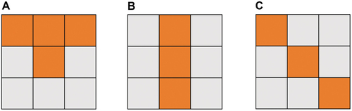
The original HiTS procedure prioritizes the detection of high-magnitude and possibly ephemeral changes that are highly sparse across the time series (Maeng Citation2019). This characteristic is mainly related to the aggregation strategy of the detail coefficients in the HiTGUW transform and thresholding steps (Section 2.4). To detect forest patches characterized by disturbance and recovery dynamics, HILANDYN accounts for the similarity in spectral-temporal information from adjacent Landsat pixels. Indeed, within the spatial kernel, changes may occur in a subset of pixels, for example, when the focal pixel lies at the edges of a disturbed forest patch () or belongs to a linear feature (). We have therefore modified the HiTS procedure to fully exploit the spectral information in the spatial neighborhood included in high-dimensional Landsat time series.
Figure 3. Examples of the spatial arrangement of disturbed pixels (orange) within the spatial kernel used by HILANDYN where the focal pixel is surrounded by non-disturbed pixels (grey).
First, in the HiTGUW transformation, we modified the aggregation strategy of the detail coefficients so that the merging order of the time intervals depends on the sum of their maximum and average. This procedure delays the merging of those time intervals that contain both large and dense deviations from linearity among the variables of the high-dimensional time series, thus favoring the detection of true changepoints in the thresholding step.
Second, in order to preserve the spatial pattern of disturbed patches, we embedded the spectral-temporal information provided by the neighboring pixels in the HiTGUW transformation. Specifically, the wavelet basis is constructed by prioritizing the detail coefficients of those neighboring pixels that are more similar to the focal pixel, taking into account the spectral and temporal characteristics. In particular, for each band, we computed the spectral angle mapper (SAM; EquationEquation 4(4)
(4) ; Kruse et al. Citation1993) between vectors
and
, corresponding to one neighboring and focal Landsat pixel, respectively, and having length
, i.e. the length of time series.
The weight assigned to each neighboring pixel, , falls in the interval [0, 1] and is computed as the sum of the SAM values obtained for each band (EquationEquation 5
(5)
(5) ).
Where is the number of bands and
is the number of neighboring pixels, i.e. eight.
Third, the column-wise aggregation of the detail coefficient matrix in the thresholding step of the HiTS procedure is performed using two alternative strategies, depending on which one produces the highest aggregated detail coefficient. One approach is based on the mean of the detail coefficients relative to all the
variables in the high-dimensional time series, where each band is weighted using the pixel-wise weights, computed as in EquationEquation 5.
(5)
(5) The alternative approach involves computing the mean of the detail coefficients considering only the bands in the focal pixel. HILANDYN can use these two approaches interchangeably, as the threshold for evaluating the significance of the deviation from linearity depends solely on the number of bands included in the high-dimensional time series (EquationEquation 3
(3)
(3) ). Finally, we applied the finite sample bias correction factor proposed by Park et al. (Citation2019) to the MAD (EquationEquation 2
(2)
(2) ) to improve the estimation of the standard deviation.
2.6. Noise filter
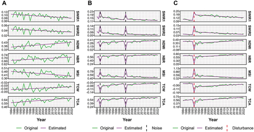
HILANDYN typically ignores impulsive noise caused by artifacts in reflectance composites when it is sparse among the time series () thanks to the modifications to the HiTS procedure. Nevertheless, changepoints caused by dense impulsive noise () can be confounded with those associated with real changes such as forest disturbances (). Therefore, we designed a two-stage noise filter that is iteratively applied to remove spurious changepoints (). At each iteration, the noise filter first identifies candidate changepoints, i.e. changepoints potentially caused by impulsive noise, and then processes them. The activation of the noise filter and the maximum number of iterations allowed for processing impulsive noise are controlled through the parameter.
Figure 4. Example of time series of three focal pixels containing sparse noise (a), dense noise (b) or spectral changes caused by a wildfire (c). HILANDYN ignored sparse noise (a) while detected the dense ones in 1986 and 2002 (b). The wildfire occurred in 1991 (c) caused a changepoint characterised by a spike similar to impulsive noise though some bands, i.e. SWIR1, SWIR2 and TCW, did not exhibit a rapid spectral recovery.
During the initial stage (), the noise filter searches for spurious changepoints by analyzing individual intervals, , which include one or multiple consecutive changepoints and the preceding time point. When
is at the beginning of the time series, HILANDYN evaluates the reliability of changepoints in the interval through condition
(EquationEquation 6
(6)
(6) , ).
Figure 5. Diagram of the operations performed by the noise filter during the screening stage for each interval. The number of observations per year and the parameter are required for evaluating condition
. Original and estimated spectral values are required for evaluating conditions
and
. Time points at the beginning of the time series are first processed through condition
. Conditions
and
are checked on time points that exhibit the maximal spectral deviation from a reference value. Blue boxes indicate input data, black boxes indicate processing and green boxes indicate outputs.
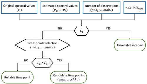
Where and
are the number of observations available at
and
, and
is a constant corresponding to the minimum number of clear observations required for producing reflectance composites. The number of clear observations available for each time point is computed as the median of the per-pixel clear observations within the spatial kernel. The value assigned to
should maximize the reliability of reflectance composites while not exceeding the maximum number of observations theoretically available for a given location and time period. Therefore,
primarily depends on the compositing approach, on the temporal frequency of Landsat data at the beginning of the time series, i.e. 8 or 16 days, and whether the study area is located where Landsat tiles overlap.
When condition is not satisfied, the noise filter finds a time point,
, in each band, whose values in the spatial kernel differ the most from the reference ones. For a single band, given a set of
vectors,
=
, where
, with
corresponding to the number of pixels in the spatial kernel, the noise filter finds the vector
that maximizes the Euclidean distance to the reference vector
(EquationEquation 7
(7)
(7) ).
Where denotes the Euclidean norm and
contains the spectral values estimated by the HiTS procedure at the time point preceding
or at that following
, depending on the position of
. The vectors in the set
contain values fitted through the HiTS procedure except for
, which contains original input values.
A time point becomes a candidate time point,
, if at least one band at that location satisfies both conditions
(EquationEquation 8
(8)
(8) ) and
(EquationEquation 9
(9)
(9) ).
where , with
corresponding to the number of pixels within the spatial kernel, and
is the sign function.
Condition (EquationEquation 8
(8)
(8) ) requires that the spectral distance between the time points preceding and following
is lower than that between
and the following time point. Condition
(EquationEquation 9
(9)
(9) ) requires that at least one pixel in the spatial kernel has to form a spike at
.
During the processing stage, the noise filter analyzes candidate time points individually, by iteratively reprocessing a subset of the high-dimensional time series (). The algorithm removes all the data at and selects the variables relative to those bands that exhibited a significant change. Specifically, we deemed a changepoint in a specific band significant if the number of changed pixels within the spatial kernel is equal to or greater than the median number of changed pixels among all the bands. A changepoint is labeled as an actual change if a new changepoint is detected at the beginning of the interval. Spectral values within unreliable intervals are replaced with the average of the two observations following the interval, while time points associated with spurious changepoints are replaced through linear interpolation.
2.7. Accuracy assessment
Our definition of forest disturbance was as broad as possible and included changes associated with either stand-replacing, e.g. high-severity crown fires and windthrows, or non-stand-replacing events, e.g. drought-induced mortality and defoliating insect outbreaks. We considered individual events in space, i.e. at the scale of a Landsat pixel, and time, i.e. per year, following other studies (Bullock, Woodcock, and Holden Citation2020; Cohen et al. Citation2017). Therefore, we treated consecutive disturbances, e.g. windthrows followed by salvage logging, as separate events. Our validation dataset included 3000 plots (, ), each corresponding to a Landsat pixel, that were forested at any time during the analysis period. To locate validation plots, we used a stratified random sampling based on two strata delineated for each disturbed patch detected using an initial version of HILANDYN. Each stratum corresponded to either detected disturbed patches, i.e. the inner stratum, or a two-pixel positive buffer around these patches, i.e. the outer stratum. We classified disturbance events as stand-replacing or non-stand-replacing using the relative TCW change magnitude and a threshold of 50%, as proposed by Cohen et al. (Citation2018). The number of stand-replacing disturbance events in the inner stratum was noticeably higher than that in the outer stratum (, Figure S2).
Table 2. Information on the validation dataset based on the validation strata. We discriminated between stand-replacing and non-stand-replacing events using a threshold of 50% of the relative TCW change magnitude.
Using a buffer stratum was recommended for applications involving classifying rare phenomena such as forest disturbances (Olofsson et al. Citation2020). To discriminate between noise and disturbances, we considered only those events that occurred until the second-last year of the time series, i.e. until 2021.
Operationally, one operator determined the occurrence of a disturbance by simultaneously visualizing temporal profiles of annual Landsat time series at the plot-level and raster data in QGIS software, using the RasterDataPlotting and RasterTimeseriesManager plugins (https://raster-data-plotting.readthedocs.io/en/latest/index.html). Raster data comprised RGB false-color composites derived from Landsat yearly reflectance data (R = SWIR2, G = NIR, B = Red), nationwide aerial orthophotos, and high-resolution satellite imagery provided free-of-charge by Google, Bing, and Esri. By evaluating individual years for each plot, we obtained 111,000 sample units, of which 2802 were disturbance events as some plots were disturbed multiple times. Using a confusion matrix, we computed three accuracy metrics relative to the disturbed class: user’s accuracy (UA; EquationEquation 10(10)
(10) ), i.e. precision, producer’s accuracy (PA; EquationEquation 11
(11)
(11) ), i.e. recall, and F1 score (EquationEquation 12
(12)
(12) ).
2.8. Algorithm parametrization
HILANDYN requires a few parameters for processing high-dimensional Landsat time series. The primary ones are the bands to include in the time series and the constant factor (EquationEquation 3
(3)
(3) ). The constant factor
and the number of bands influence the threshold λ (Figure S1; Section 2.5), which controls the sensitivity toward deviations from linearity in the HiTS procedure. Furthermore, the selection of bands is crucial as they are characterized by different sensitivities to forest disturbances (Cohen et al. Citation2018; DeVries et al. Citation2016; Schultz et al. Citation2016). We assessed how the parameters required by HILANDYN () affected the accuracy metrics across the two validation strata (Section 2.7). Specifically, we first searched for the best performing combination of input bands () and constant
in terms of F1 score and then tested the parameters for configuring the noise filter. The latter is controlled by the parameters
and
(Section 2.6).
Table 3. List of the main parameters required by HILANDYN and values tested for the sensitivity analysis.
2.9. Comparison with BEAST
We selected BEAST (Zhao et al. Citation2019) to perform a comparison with HILANDYN based on our validation dataset. BEAST builds additive models by considering time series as linear combinations of seasonality, trend, abrupt changes, and noise, similar to BFAST (Breaks For Additive Seasonal and Trend; Verbesselt et al. Citation2010). Here, we employed the beast123 function provided in the Rbeast (version 0.9.9) R package to analyze the annual Landsat time series (Section 2.2) that included data from the spatial and spectral dimensions. Specifically, we tested time series that included data relative to one band and one pixel, one band and nine pixels, i.e. within a three-by-three spatial kernel, multiple bands and one pixel, and multiple bands and nine pixels. Input time series included either NBR due to its effectiveness in disturbance detection, e.g. Cohen et al. (Citation2020), or those bands that achieved the best F1 score in the sensitivity analysis of HILANDYN (Section 2.8).
Since our time series have annual frequency, we excluded the seasonal component, forcing BEAST to estimate linear trends, i.e. a polynomial order of one. As pointed out by Zhao et al. (Citation2019), BEAST is sensitive to two hyperparameters: the maximum number of seasonal and trend changepoints and the minimum distance in time between two neighboring changepoints in a model. We therefore tested the maximum number of trend changepoints (trendMaxKnotNum) for values in the interval [1, 10], while we set 1 year as the minimum distance in time between two neighboring changepoints. This latter parameter allowed us to make a direct comparison with HILANDYN. We used the pre-defined values of the algorithm for all the other parameters.
Though BEAST can handle high-dimensional time series, being a univariate algorithm, it computes the probability distributions associated with the number of trend changepoints (ncpPr) and their position in time (cpOccPr) separately for each variable. Therefore, we used the mean to summarize these probability distributions among the variables in the high-dimensional time series. To find the position of the most probable changepoints, we followed the approach proposed by the authors of the algorithm. That is, we first obtained the mean number of changepoints, ncp, using the corresponding mean probability distribution. We then selected a set of changepoints, whose number was equal to ncp, among those with the highest mean occurrence probability. Finally, we used the same approach employed by HILANDYN (Section 2.3) for identifying trend changepoints associated with disturbances.
We compared BEAST and HILANDYN in terms of computation time by including from 1 to 14 bands in the high-dimensional time series within a three-by-three spatial kernel. Each combination of bands included those that performed best with HILANDYN in terms of producer’s accuracy when the constant factor was equal to one (Table S1).
3. Results
3.1. Quantitative assessment: detection capabilities and sensitivity analysis of the parameters
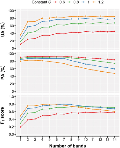
The constant factor and the number of bands included in the high-dimensional Landsat time series influenced the accuracy metrics noticeably (, Table S1). Increasing the value of
and the number of bands markedly gained UA while partly reduced PA, though this latter remained stable until the number of bands was equal or lower than seven. The highest increase in UA occurred when more than one band was included in the high-dimensional time series (, Table S1). Without the noise filter, HILANDYN achieved the highest PA (93.3%) with the constant
equal to 0.6 and seven bands in the high-dimensional time series, while it achieved the highest UA (85.5%) with
equal to 1.2 and 12 band. The algorithm achieved the highest F1 score (0.802) when we set
equal to 1 and included seven bands (, Table S1).
Figure 6. Maximum values of user’s accuracy (UA), producer’s accuracy (PA) and F1 score based on the validation dataset and computed from all the unique combinations of bands with lengths from one to 14. The value of the constant ranged from 0.6 to 1.2. The noise filter was deactivated.
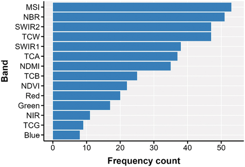
The selection of bands to include in the high-dimensional time series influenced primarily the PA, while the UA was mainly determined by their number (). Considering the results obtained with the constant factor in the interval [0.6, 1.2] and all the unique combinations of bands, seven of them were included most often in the best-performing combinations in terms of PA (). Specifically, MSI, NBR, SWIR2, TCW, SWIR1, TCA, and NDMI emerged as the most effective bands for forest disturbance detection (). Differences with the remaining bands in terms of selection frequency were noticeable.
Figure 7. Distribution of values of user’s accuracy (UA), producer’s accuracy (PA) and F1 score based on the validation dataset and computed from all the unique combinations of bands with lengths from one to 14. The value of the constant factor was equal to one. The noise filter was deactivated.
Figure 8. Frequency count relative to the number of times each band was in the best-performing combination in terms of PA, using from one to 14 bands in the high-dimensional time series. Results obtained with values of the constant factor ranging from 0.6 to 1.2 were pooled together. The noise filter was deactivated.
Using the configuration that produced the best performance in terms of F1 score, i.e. the combination of SWIR1, SWIR2, NDMI, NBR, MSI, TCW, and TCA, and equal to one (, Table S1), the noise filter significantly increased UA while marginally decreased PA (Figure S3, Table S2). Specifically, UA increased up to 9.7%, i.e. from 73.7% to 83.4%, while PA decreased up to 4.6%, i.e. from 87.8% to 83.2%. The noise filter increased the F1 score slightly, from 0.801 to 0.833 when
was equal to four and
was equal to five (Figure S3, Table S2). HILANDYN achieved a substantial balance between UA and PA when we activated the noise filter, and this was consistent across the different validation strata (). The increase in UA caused by the noise filter was greater in the outer stratum than in the inner one, with a variation of 13% and 6.6%, respectively (). Similarly, the reduction in PA caused by the noise filter was greater in the outer stratum than in the inner one, with a reduction of 6.5% and 3.3%, respectively (). HILANDYN achieved comparable accuracies in validation plots dominated by either broadleaf or conifer tree species (Table S3).
Table 4. User’s accuracy (UA), producer’s accuracy (PA), and F1 score achieved by HILANDYN with the noise filter activated or not. Accuracy metrics were computed using either both strata of the validation dataset or a single one. High-dimensional Landsat time series included data from seven bands (SWIR1, SWIR2, NDMI, NBR, MSI, TCW, and TCA) within a three-by-three spatial kernel. We parametrized the algorithm using = 1,
= 4, and
= 5.
Overall, the noise filter allowed HILANDYN to reduce the influence of spurious changepoints caused by impulsive noise, as highlighted by the decrease from 23.5% to 14.9% in the median relative TCW change magnitude of commission errors (, Table S4). For omission errors, the noise filter did not change the median relative TCW change magnitude, as this latter slightly decreased from 46.6% to 45.3% when we filtered noise (, Table S4).
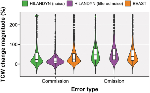
Figure 9. Distribution of the relative TCW change magnitude of commission (100 – UA) errors and omission (100 – PA) errors for HILANDYN and BEAST. High-dimensional Landsat time series included data of seven bands (SWIR1, SWIR2, NDMI, NBR, MSI, TCW and TCA) within a three-by-three spatial kernel. We parametrised each algorithm using the settings that provided the best results in terms of F1 score. We constrained the relative TCW change magnitude between −50% and 250% by assigning these values to those outside that range.
3.2. Comparison with BEAST
The accuracy of BEAST, especially the PA and F1 score, increased when we added both spectral and spatial data in the input time series ().
Table 5. User’s accuracy (UA), producer’s accuracy (PA), and F1 score achieved by BEAST with the validation dataset as a function of the maximum number of trend changepoints (trendMaxKnotNum) and the data in the time series. Input time series included either data of one band (NBR), or seven bands (SWIR1, SWIR2, NDMI, NBR, MSI, TCW, and TCA) of one or nine pixels, i.e. within a three-by-three spatial kernel. The highest value of each accuracy metric for every input data type is highlighted in bold.
In particular, the PA peaked at 85.8% and the F1 score at 0.717, when we used high-dimensional time series that included data of the seven best-performing bands in terms of PA (SWIR1, SWIR2, NDMI, NBR, MSI, TCW, and TCA; ) extracted using a three-by-three spatial kernel. The maximum number of trend changepoints markedly influenced the accuracy of BEAST as changes in its values between 1 and 10 caused significant variations of UA and PA up to approximately 23% (). In particular, the PA increased when we raised the maximum number of trend changepoints, while the UA followed the opposite trend. Therefore, we achieved the highest F1 score by setting the maximum number of trend changepoints equal to three ().
Overall, the best F1 score provided by BEAST (0.717) was lower than that provided by HILANDYN (0.801) when the noise filter was deactivated. With regard to the best F1 score, the UA achieved by BEAST (67.2%, ) was lower than that of HILANDYN (73.7%, Table S2). Similarly, differences in PA between the algorithms were noticeable, with BEAST and HILANDYN achieving 76.9% () and 87.8% (Table S2), respectively.
The distribution of commission, i.e. 100 – UA, and omission, i.e. 100 – PA, errors in terms of relative TCW change magnitude highlighted slight differences between HILANDYN and BEAST (, Table S4). The median relative TCW change magnitude of commission errors was 23.5% for HILANDYN (noise filter deactivated) and 25.1% for BEAST. Conversely, for omission errors, these values were 46.6% for HILANDYN (noise filter deactivated) and 37.6% for BEAST.
BEAST required considerably more time to process Landsat time series of the validation dataset compared to HILANDYN (, Table S5).
Figure 10. Execution time required by HILANDYN and BEAST to process the 39-year high-dimensional time series of the validation dataset. The total number of variables in each time series was equal to the product of the number of bands and nine, i.e. the number of pixels within a three-by-three spatial kernel. The bands selected in each combination were those that gave the best results in terms of PA with HILANDYN when the constant was equal to one (Table S1). We configured the noise filter of HILANDYN by setting the
to four and
to five. For BEAST, we used the predefined prior parameters except for trendMaxknotnum and trendMinsepdist that we set to eight and one, respectively. Each process ran on a single core of an AMD Ryzen 9 5950X processor.
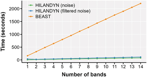
In particular, differences between the two algorithms increased with the number of bands in high-dimensional time series, as BEAST required proportionally higher computational time compared to HILANDYN. For instance, processing high-dimensional time series with 63 variables, i.e. the values of seven bands extracted from nine connected pixels, required 40 and 1117 seconds for HILANDYN and BEAST, respectively (, Table S5). When we activated the noise filter, the computation time required by HILANDYN increased to 64 seconds.
3.3. Qualitative assessment of the detection capabilities
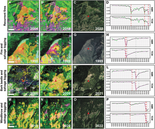
HILANDYN was sensitive to a wide range of disturbance severities as it detected forest patches disturbed by stand-replacing events, such as wildfires, windthrow, and sleet damage, and non-stand-replacing events, such as tree crown dieback caused by defoliating insects and severe drought and heat waves (). The spatio-temporal pattern of disturbed forest patches detected by HILANDYN exhibited a high degree of contiguity among pixels, which was consistent across different disturbance agents and severities (). Moreover, HILANDYN effectively detected forest patches that were repeatedly disturbed, either a few years apart or in close succession, i.e. one year apart (). Secondary disturbances occurring shortly after the main event were often associated with salvage logging in our study area. In particular, the temporal profiles of NBR and TCW highlighted different sensitivities to the complete removal of tree cover associated with salvage logging when it occurred shortly after the natural disturbance ().
Figure 11. Examples of stand-replacing and non-stand-replacing forest disturbances detected by HILANDYN in the study area between 1985 and 2022. Panels A-F depict the following disturbance events: (a) dieback induced by defoliating insect outbreak (Asian chestnut gall wasp, Dryocosmus kuriphilus) in 2011; (b) dieback caused by a severe drought and heatwave in 2003; (c) wildfires in 1990, 1991, 2003, and 2017; (d) windthrow in 2007; (e) ice storm in 2014; (f) windthrow in 2018. The grey background in the central panel indicates the presence of forest cover either in 1990 or 2018 according to the Corine Land Cover within the European Alps borders (blue line).
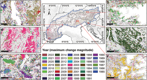
Figure 12. Examples of disturbed forest patches detected by HILANDYN and characterised by different disturbance agents and severities. Please refer to the legend in for the colour corresponding to each year in panels a-e. Clearcuts (a, f; 5°45‘18,102“E; 44°3’9,791“N), debris flows (b, g; 8°1‘54,389“E; 46°46’4,057“N), defoliating insect outbreak (c, h; 7°35‘10,709“E; 45°22’18,178“N), wildfire (d, i; 13°16‘54,707“E; 46°28’25,202“N), windthrow (e, j; 7°21‘17,61“E; 44°39’31,641“N). The grey background indicates the presence of forest cover either in 1990 or 2018 according to the Corine Land Cover.
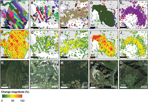
Figure 13. Examples of forest patches, depicted in yellow, that were disturbed multiple times during the analysis period. Each row shows results from HILANDYN, recent high-resolution satellite imagery, and temporal profiles of NBR and TCW. We parametrised the algorithm according to the configuration that achieved the highest F1 score (Section 3.1). Recurrent wildfires (a-d; 7° 9’1.02“E; 45° 9’35.57“N). Wildfire followed by salvage logging (e-h; 9°39’23.26“E; 46°11’59.51“N). Bark beetle attack followed by salvage logging (i-l; 14°42’0.63“E; 46°16’1.43“N). Windthrow followed by salvage logging (m-p; 11°21’13.93“E; 46°17’41.66“N).
4. Discussion
4.1. Key features of HILANDYN
Here, we presented a novel, unsupervised algorithm for retrospectively mapping forest disturbance dynamics, although its capabilities are not limited to any specific land cover. In the context of Landsat time series-based algorithms, the novelty introduced by HILANDYN lies in its ability to temporally segment high-dimensional Landsat time series containing multispectral information from adjacent pixels. By integrating information from the spectral and spatial domains into the time series, HILANDYN was able to achieve satisfactory accuracy () while providing spatio-temporal consistency of disturbed forest patches (). These results are made possible by the modified HiTS procedure, which provides a computationally sound approach to reduce the dimensionality of high-dimensional time series in the early stages of the analysis. The construction of a unique, data-driven wavelet basis from all the variables in the time series (Section 2.4) and the aggregation strategy of the detail coefficients (Section 2.5) are key elements for detecting changepoints by exploiting the spectral and spatial domains. Widely used algorithms that can harness information from multiple bands, such as CCDC (Zhu and Woodcock Citation2014) and COLD (Zhu et al. Citation2019), primarily work in parallel, processing data in a band-wise manner and combining univariate tests to detect changepoints in later stages of the analysis. This results in high computational requirements and the need to run the algorithms on geospatial cloud computing platforms, such as Google Earth Engine, to analyze large areas (Bullock, Woodcock, and Holden Citation2020; Pasquarella et al. Citation2022).
Algorithms designed to exploit the spatial correlation between adjacent pixels via OBIA, e.g. VeRDET (Hughes, Kaylor, and Hayes Citation2017) and OB-COLD (Ye, Zhu, and Cao Citation2023), typically perform temporal segmentation either after or before the spatial analysis. In addition to increasing computational and algorithmic complexity, sequential approaches require appropriate parametrization for each stage of the analysis, such as setting the optimal scale for spatial segmentation. Conversely, the inclusion of spectral information from the spatial context in high-dimensional time series enhanced the capabilities of HILANDYN by extending the spatial scale of the analysis without increasing the number of parameters. Indeed, the pixel-wise weighting scheme and the thresholding approach in the modified HiTS procedure (Section 2.5) allowed the algorithm to take advantage of the spatial context while maintaining its sensitivity to changes occurring at the individual Landsat pixel.
The bottom-up, i.e. agglomerative, approach employed by the HiTS procedure to construct the adaptive wavelet basis has proved to be effective for the temporal segmentation of high-dimensional time series, as demonstrated by the accuracy metrics achieved by HILANDYN (). When applied to the segmentation of different types of signals, bottom-up approaches outperform those based on sliding windows and top-down algorithms (Keogh et al. Citation2004). They have also been successfully used for temporal segmentation in other Landsat time series-based algorithms, such as in C2C (Hermosilla et al. Citation2015). The HiTGUW transformation, i.e. the first stage of the HiTS procedure, focuses on local features in its early stages before identifying global features, which enables HILANDYN to perform well in detecting abrupt local changes, including point anomalies, e.g. , and consecutive disturbances occurring in close succession, e.g. . Bottom-up temporal segmentation also proved to be useful in the first stage of the noise filter built into HILANDYN, i.e. to find changepoints potentially caused by spectral noise. Indeed, when the noise filter was activated, the UA increased significantly () and the change magnitude associated with commission errors decreased ().
4.2. Algorithm parametrization
HILANDYN proved to scale well to a considerably large study area when configured with a single set of parameters that maximized the F1 score (, ). Indeed, we achieved an overall balance between UA and PA while detecting forest patches disturbed by different agents and a wide range of severity. Landsat time series-based algorithms typically require to fine-tune the main parameters to adapt to different study areas (Pasquarella et al. Citation2022) and specific disturbance agents (Ye et al. Citation2021). HILANDYN mostly missed non-stand-replacing events when using the best performing set of parameters, as shown by the relative TCW change magnitude for omission errors (, Table S4). This behavior is common among Landsat time series-based automated algorithms, as the detection of low-severity disturbances is typically hindered by residual spectral noise in Landsat time series (Cohen et al. Citation2017; Rodman et al. Citation2021). Nevertheless, the high PA achieved by HILANDYN in the outer validation stratum, i.e. 78.9% with the noise filter deactivated (), evidenced its overall sensitivity to non-stand-replacing events.
Since the threshold used by the modified HiTS procedure depends directly on the number of bands and the constant
(EquationEquation 3
(3)
(3) ), the optimization of these parameters is critical to discriminate between low-severity disturbances and spurious changepoints. In fact, increasing the value of
reduces the sensitivity of HILANDYN to low-severity disturbances, which are typically characterized by small and transient deviations from linearity in the linear trends. It is worth noting that the optimization of
in HILANDYN allows the user to maximize the balance between UA and PA (, Table S1), thus reducing the need to post-process the disturbance metrics generated by the algorithm. In contrast, other temporal segmentation algorithms such as LandTrendr, C2C, and BEAST require setting a predefined maximum number of changepoints or linear segments.
When we included the best performing bands in the high-dimensional time series, their number and the constant had a significant effect on UA, whereas PA was less sensitive to their variations (, Table S1). As observed with other Landsat time series-based algorithms, such as LandTrendr (Cohen et al. Citation2018, Citation2020; Pasquarella et al. Citation2022) and COLD (Cohen et al. Citation2020), the use of a single band introduces a significant amount of uncertainty in temporal segmentation, primarily due to increased commission errors. The heterogeneity of spectral changes across wavelengths associated with disturbance events (Pasquarella et al. Citation2022), and the difficulty of effectively distinguishing between low-severity disturbances and noise are the main sources of uncertainty. Secondary classification models that combine the results of multispectral ensembles obtained from univariate algorithms, e.g. LandTrendr, were primarily aimed to increase UA of disturbance maps (Cohen et al. Citation2018, Citation2020; Senf and Seidl Citation2020). HILANDYN benefited from the increase in the number of bands in terms of UA (; ) because this likely reduced the influence of band-dependent noise, as shown in . The latter can be caused by several factors, such as the presence of cirrus clouds, which alter the surface reflectance unevenly across wavelengths, with a smaller effect on the SWIR bands than on the others (Qiu, Zhu, and Woodcock Citation2020). Conversely, forest disturbances and band-independent noise typically cause dense changes in high-dimensional time series () and further processing is required to correctly separate them (Section 2.6).
Regarding the selection of bands, their effectiveness in detecting forest disturbances largely depends on the residual information they carry after the normalization by the estimated standard deviation of the random error (EquationEquation 3
(3)
(3) ). In this study, the best-performing bands in terms of PA () were seven and, except for TCA, they were based on the SWIR wavelengths, either the original reflectance bands, i.e. the SWIR2 and SWIR1 bands of the Landsat sensors, or the spectral indices contrasting the NIR and the SWIR bands (MSI, NBR, TCW, and NDMI). The effectiveness of the SWIR bands for forest disturbance detection has been reported for different forest ecosystems and different change detection algorithms (Cohen et al. Citation2018; DeVries et al. Citation2016; Hislop et al. Citation2019). In particular, algorithms that use one image per year appear to rely mostly on SWIR bands to detect forest disturbance (Cohen et al. Citation2018, Citation2020). Conversely, algorithms that fit harmonic functions to all the available Landsat images, such as COLD, rely primarily on information in the NIR band due to its effectiveness in reconstructing forest phenology (Cohen et al. Citation2020). Results in also highlighted the usefulness of the TCA band, as it complemented the information provided by the SWIR-based bands. Consistent with previous studies (Cohen et al. Citation2018, Citation2020), our results showed that TCA outperformed the widely used NDVI in detecting forest disturbances when using one image per year due to its greater sensitivity at high levels of vegetation cover (Cohen et al. Citation2016).
Optimizing the two parameters required by the integrated noise filter, i.e. and
, further improved the balance between UA and PA (Table S2, Figure S4), as HILANDYN effectively discriminated between noise and trustworthy changes (, ). The
parameter is aimed to reduce over-segmentation at the beginning of the time series, which is caused by residual noise in the reflectance composites due to data scarcity. Indeed,
strictly depends on the compositing algorithm, as this latter can significantly affect the quality of the reflectance composites (Qiu et al. Citation2023).
4.3. Comparison with BEAST
Despite being a univariate algorithm, BEAST benefited from the use of multispectral information and from the inclusion of spatial context information in the time series, achieving the best results when we combined this information (). In fact, increasing the number of variables in high-dimensional time series increased both UA and PA to values similar to those achieved by HILANDYN (Section 3.1). Nevertheless, BEAST struggled to achieve a balance between UA and PA, as evidenced by the relatively low F1 score (). This was determined by the strong dependence of UA and PA on the maximum number of trend changepoints, which are inversely correlated with this parameter. In particular, the relatively low UA achieved by BEAST, i.e. around 55% or less, when we set the maximum number of trend changepoints higher than three (), seems to confirm the larger proportion of commission over omission errors initially reported by Zhao et al. (Citation2019). The analysis of the relative TCW change magnitude associated with commission and omission errors showed that BEAST and HILANDYN had comparable sensitivity to disturbances in terms of severity (, Table S4). Nevertheless, the relative TCW change magnitude of omission errors evidenced that BEAST was slightly more sensitive to non-stand-replacing events compared to HILANDYN (, Table S4). This highlighted the effectiveness of the Bayesian approach in detecting subtle trend changepoints in Landsat time series. Overall, the main limitations associated with this approach stem primarily from the significant computing power required, which increases linearly with the number of variables included in the time series (). This can be a significant challenge for applications over large areas or when using high spatial resolution data, unless high-performance computing platforms are used.
4.4. Limitations and future developments
Compared to other Landsat time series-based algorithms, such as BFAST Monitor (DeVries et al. Citation2015) and COLD (Zhu et al. Citation2019), we developed HILANDYN to analyze forest disturbance dynamics retrospectively. Therefore, the algorithm lacks crucial features dedicated to real-time monitoring . First, the HiTS procedure is a complete offline approach; thus, a reanalysis of the entire time series is required when new data is added. A possible solution could come from online approaches such as SWAB (Keogh et al. Citation2001), which combine sliding windows and bottom-up methods by applying the latter within sliding windows of constant size . Notably, a sliding window approach has been adopted by Mulverhill et al. (Citation2023) to add monitoring capabilities to BEAST. We note that online algorithms, such as CCDC and COLD, need to reinitialize the time series model after a disturbance event, which may result in the omission of consecutive disturbances occurring in close succession. For this reason, backward fitting of the data has been proposed after a disturbance event for the OB-COLD algorithm (Ye, Zhu, and Cao Citation2023).
Second, the annual frequency of the time series employed by HILANDYN hinders the timely detection of forest disturbances, which is a fundamental requirement for monitoring purposes. While using time series with evenly spaced observations is required by the HiTS procedure, seasonal reflectance composites could increase the number of observations available during the year, as proposed by some studies based on LandTrendr (Meng et al. Citation2021). Similarly, approaches for normalizing phenological variations offer the opportunity to model intra-annual time series through linear trends (Yang et al. Citation2023). An increase in the temporal frequency of high-dimensional time series from inter- to intra-annual would also limit the reduction in PA caused by the noise filter (). A higher temporal frequency would reduce the omission of low-severity disturbances caused by the masking effect of post-disturbance vegetation recovery (Yang et al. Citation2023). However, Giannetti et al. (Citation2021) reported that the optimal time interval required to achieve the highest accuracy of disturbance maps, regardless of the algorithm, was between 7 and 12 months.
Third, linear trends may be suboptimal for modeling satellite time series as nonlinear trends may be better suited to represent forest dynamics (Moisen et al. Citation2016; Senf, Müller, and Seidl Citation2019). A possible improvement to HILANDYN could be the extension to piecewise-quadratic signals, as proposed by Maeng and Fryzlewicz (Citation2023) for the TrendSegment procedure, i.e. the univariate version of the HiTS procedure. Nevertheless, changes in linear trends have been found to be useful for detecting non-stand-replacing disturbances and forest dieback in general (Moreno-Fernández et al. Citation2021; Mulverhill, Coops, and Achim Citation2023).
5. Conclusions
As changes in disturbance regimes are critical to understand the effects of climate change on forest ecosystems, automated and accurate methods are needed to reconstruct regional-scale forest disturbance dynamics from long-term satellite time series. HILANDYN offers new opportunities to study forest disturbance dynamics retrospectively by exploiting the temporal, spatial, and spectral domains provided by Landsat data. In fact, temporal segmentation of high-dimensional time series through the modified HiTS procedure is the key element of our algorithm. It ensures an accurate detection of disturbance events and guarantees computational efficiency by reducing the dimensionality of the time series in the early stages of the processing by locating deviations from linearity that are common between variables. The comparison with BEAST confirms the robustness of HILANDYN for the detection of stand-replacing and non-stand-replacing disturbances. Its scalability to large study areas is supported by the high computational efficiency and flexibility to heterogeneous conditions when using a single set of parameters. The methods implemented in HILANDYN are general enough to analyze time series of optical satellite imagery other than Landsat, such as that acquired by the Sentinel-2 satellites.
Supplementary material R1.docx
Download MS Word (285.1 KB)Acknowledgments
We acknowledge the U.S. Geological Survey for distributing Landsat imagery and Dr Andreas Rabe for providing the Raster Timeseries Manager plugin for QGIS.
Disclosure statement
No potential conflict of interest was reported by the author(s).
Data availability statement
The code of the algorithm is implemented in the R package “hilandyn” publicly available via the GitHub repository of the first author at https://github.com/donatomorresi/hilandyn.
Supplementary material
Supplemental data for this article can be accessed online at https://doi.org/10.1080/15481603.2024.2365001
Additional information
Funding
References
- Allen, C. D., D. D. Breshears, and N. G. McDowell. 2015. “On Underestimation of Global Vulnerability to Tree Mortality and Forest Die-Off from Hotter Drought in the Anthropocene.” Ecosphere 6 (8): 1–25. https://doi.org/10.1890/ES15-00203.1.
- Allen, C. D., A. K. Macalady, H. Chenchouni, D. Bachelet, N. McDowell, M. Vennetier, T. Kitzberger, et al. 2010. “A Global Overview of Drought and Heat-Induced Tree Mortality Reveals Emerging Climate Change Risks for Forests.” Forest Ecology & Management 259 (4): 660–684. https://doi.org/10.1016/j.foreco.2009.09.001.
- Andrus, R. A., R. K. Chai, B. J. Harvey, K. C. Rodman, T. T. Veblen, and G. Battipaglia. 2021. “Increasing Rates of Subalpine Tree Mortality Linked to Warmer and Drier Summers.” The Journal of Ecology 109 (5): 2203–2218. https://doi.org/10.1111/1365-2745.13634.
- Banskota, A., N. Kayastha, M. J. Falkowski, M. A. Wulder, R. E. Froese, and J. C. White. 2014. “Forest Monitoring Using Landsat Time Series Data: A Review.” Canadian Journal of Remote Sensing 40 (5): 362–384. https://doi.org/10.1080/07038992.2014.987376.
- Bebi, P., R. Seidl, R. Motta, M. Fuhr, D. Firm, F. Krumm, M. Conedera, C. Ginzler, T. Wohlgemuth, and D. Kulakowski. 2017. “Changes of Forest Cover and Disturbance Regimes in the Mountain Forests of the Alps.” Forest Ecology and Management 388:43–56. https://doi.org/10.1016/j.foreco.2016.10.028.
- Brooks, E. B., R. H. Wynne, V. A. Thomas, C. E. Blinn, and J. W. Coulston. 2014. “On-The-Fly Massively Multitemporal Change Detection Using Statistical Quality Control Charts and Landsat Data.” IEEE Transactions on Geoscience and Remote Sensing: A Publication of the IEEE Geoscience and Remote Sensing Society 52 (6): 3316–3332. https://doi.org/10.1109/TGRS.2013.2272545.
- Brown, R. L., J. Durbin, and J. M. Evans. 1975. “Techniques for Testing the Constancy of Regression Relationships Over Time.” Journal of the Royal Statistical Society Series B Statistical Methodology 37 (2): 149–163. https://doi.org/10.1111/j.2517-6161.1975.tb01532.x.
- Bullock, E. L., C. E. Woodcock, and C. E. Holden. 2020. “Improved Change Monitoring Using an Ensemble of Time Series Algorithms.” Remote Sensing of Environment 238:111165. https://doi.org/10.1016/j.rse.2019.04.018.
- Camarero, J. J., A. Gazol, G. Sangüesa-Barreda, J. Oliva, S. M. Vicente-Serrano, and D. Gibson. 2015. “To Die or Not to Die: Early Warnings of Tree Dieback in Response to a Severe Drought.” The Journal of Ecology 103 (1): 44–57. https://doi.org/10.1111/1365-2745.12295.
- Cho, H., C. Kirch, J. Lin, I. M. Paul, L. L. Birch, J. S. Savage, and M. E. Marini. 2021. “Constructing a Polygenic Risk Score for Childhood Obesity Using Functional Data Analysis.” Econometrics and Statistics 25:66–86. https://doi.org/10.1016/j.ecosta.2021.10.008.
- Cohen, W. B., S. P. Healey, Z. Yang, S. V. Stehman, C. K. Brewer, E. B. Brooks, N. Gorelick, et al. 2017. “How Similar are Forest Disturbance Maps Derived from Different Landsat Time Series Algorithms?” Forests 8 (4): 1–19. https://doi.org/10.3390/f8040098.
- Cohen, W. B., S. P. Healey, Z. Yang, Z. Zhu, and N. Gorelick. 2020. “Diversity of Algorithm and Spectral Band Inputs Improves Landsat Monitoring of Forest Disturbance.” Remote Sensing 12 (10): 1–15. https://doi.org/10.3390/rs12101673.
- Cohen, W. B., Z. Yang, S. P. Healey, R. E. Kennedy, and N. Gorelick. 2018. “A LandTrendr Multispectral Ensemble for Forest Disturbance Detection.” Remote Sensing of Environment 205:131–140. https://doi.org/10.1016/j.rse.2017.11.015.
- Cohen, W. B., Z. Yang, S. V. Stehman, T. A. Schroeder, D. M. Bell, J. G. Masek, C. Huang, and G. W. Meigs. 2016. “Forest Disturbance Across the Conterminous United States from 1985–2012: The Emerging Dominance of Forest Decline.” Forest Ecology and Management 360:242–252. https://doi.org/10.1016/j.foreco.2015.10.042.
- Crist, E. P. 1985. “A TM Tasseled Cap Equivalent Transformation for Reflectance Factor Data.” Remote Sensing of Environment 17 (3): 301–306. https://doi.org/10.1016/0034-4257(85)90102-6.
- DeVries, B., A. K. Pratihast, J. Verbesselt, L. Kooistra, M. Herold, and K. P. Vadrevu. 2016. “Characterizing Forest Change Using Community-Based Monitoring Data and Landsat Time Series.” PLOS ONE 11 (3): e0147121. https://doi.org/10.1371/journal.pone.0147121.
- DeVries, B., J. Verbesselt, L. Kooistra, and M. Herold. 2015. “Robust Monitoring of Small-Scale Forest Disturbances in a Tropical Montane Forest Using Landsat Time Series.” Remote Sensing of Environment 161:107–121. https://doi.org/10.1016/j.rse.2015.02.012.
- European Environment Agency. 2016. “Biogeographical Regions [WWW Document]. https://www.eea.europa.eu/data-and-maps/data/biogeographical-regions-europe-3.
- European Environmental Agency. 2020. “Copernicus Land Monitoring Service – Dominant Leaf Type 2018 [WWW Document]. URL https://land.copernicus.eu/pan-european/high-resolution-layers/forests/dominant-leaf-type.( Accessed June 1, 2021).
- Foga, S., P. L. Scaramuzza, S. Guo, Z. Zhu, R. D. Dilley, T. Beckmann, G. L. Schmidt, J. L. Dwyer, M. Joseph Hughes, and B. Laue. 2017. “Cloud Detection Algorithm Comparison and Validation for Operational Landsat Data Products.” Remote Sensing of Environment 194:379–390. https://doi.org/10.1016/j.rse.2017.03.026.
- Forzieri, G., M. Girardello, G. Ceccherini, J. Spinoni, L. Feyen, H. Hartmann, P. S. A. Beck, et al. 2021. “Emergent Vulnerability to Climate-Driven Disturbances in European Forests.” Nature Communications 12 (1): 1–12. https://doi.org/10.1038/s41467-021-21399-7.
- Frantz, D., A. Röder, M. Stellmes, and J. Hill. 2017. “Phenology-Adaptive Pixel-Based Compositing Using Optical Earth Observation Imagery.” Remote Sensing of Environment 190:331–347. https://doi.org/10.1016/j.rse.2017.01.002.
- García, M. J. L., and V. Caselles. 1991. “Mapping Burns and Natural Reforestation Using Thematic Mapper Data.” Geocarto International 6 (1): 31–37. https://doi.org/10.1080/10106049109354290.
- Giannetti, F., M. Pecchi, D. Travaglini, S. Francini, G. D’amico, E. Vangi, C. Cocozza, and G. Chirici. 2021. “Estimating Vaia Windstorm Damaged Forest Area in Italy Using Time Series Sentinel-2 Imagery and Continuous Change Detection Algorithms.” Forests 12 (6): 1–16. https://doi.org/10.3390/f12060680.
- Gómez, C., J. C. White, and M. A. Wulder. 2011. “Characterizing the State and Processes of Change in a Dynamic Forest Environment Using Hierarchical Spatio-Temporal Segmentation.” Remote Sensing of Environment 115 (7): 1665–1679. https://doi.org/10.1016/j.rse.2011.02.025.
- Groen, J. J. J., G. Kapetanios, and S. Price. 2013. “Multivariate Methods for Monitoring Structural Change.” Journal of Applied Econometrics 28 (2): 250–274. https://doi.org/10.1002/jae.1272.
- Hampel, F. R. 1974. “The Influence Curve and Its Role in Robust Estimation.” Journal of the American Statistical Association 69 (346): 383–393. https://doi.org/10.1080/01621459.1974.10482962.
- Hamunyela, E., J. Verbesselt, and M. Herold. 2016. “Using Spatial Context to Improve Early Detection of Deforestation from Landsat Time Series.” Remote Sensing of Environment 172:126–138. https://doi.org/10.1016/j.rse.2015.11.006.
- Healey, S. P., W. B. Cohen, Z. Yang, C. Kenneth Brewer, E. B. Brooks, N. Gorelick, A. J. Hernandez, et al. 2018. “Mapping Forest Change Using Stacked Generalization: An Ensemble Approach.” Remote Sensing of Environment 204:717–728. https://doi.org/10.1016/j.rse.2017.09.029.
- Hermosilla, T., M. A. Wulder, J. C. White, N. C. Coops, and G. W. Hobart. 2015. “An Integrated Landsat Time Series Protocol for Change Detection and Generation of Annual Gap-Free Surface Reflectance Composites.” Remote Sensing of Environment 158:220–234. https://doi.org/10.1016/j.rse.2014.11.005.
- Hislop, S., S. Jones, M. Soto-Berelov, A. Skidmore, A. Haywood, and T. H. Nguyen. 2019. “A Fusion Approach to Forest Disturbance Mapping Using Time Series Ensemble Techniques.” Remote Sensing of Environment 221:188–197. https://doi.org/10.1016/j.rse.2018.11.025.
- Hughes, M. J., S. D. Kaylor, and D. J. Hayes. 2017. “Patch-Based Forest Change Detection from Landsat Time Series.” Forests 8 (5): 1–22. https://doi.org/10.3390/f8050166.
- Hu, T., E. Myers Toman, G. Chen, G. Shao, Y. Zhou, Y. Li, K. Zhao, and Y. Feng. 2021. “Mapping Fine-Scale Human Disturbances in a Working Landscape with Landsat Time Series on Google Earth Engine.” ISPRS Journal of Photogrammetry and Remote Sensing 176:250–261. https://doi.org/10.1016/j.isprsjprs.2021.04.008.
- Hunt, E. R., Jr, and B. N. Rock. 1989. “Detection of Changes in Leaf Water Content Using Near-And Middle-Infrared Reflectances.” Remote Sensing of Environment 30 (1): 43–54. https://doi.org/10.1016/0034-4257(89)90046-1.
- Isotta, F. A., C. Frei, V. Weilguni, M. Perčec Tadić, P. Lassègues, B. Rudolf, V. Pavan, et al. 2014. “The Climate of Daily Precipitation in the Alps: Development and Analysis of a High-Resolution Grid Dataset from Pan-Alpine Rain-Gauge Data.” International Journal of Climatology 34 (5): 1657–1675. https://doi.org/10.1002/joc.3794.
- Jirak, M. 2015. “Uniform Change Point Tests in High Dimension.” Annals of Statistics 43 (6): 2451–2483. https://doi.org/10.1214/15-AOS1347.
- Johnstone, J. F., C. D. Allen, J. F. Franklin, L. E. Frelich, B. J. Harvey, P. E. Higuera, M. C. Mack, et al. 2016. “Changing Disturbance Regimes, Ecological Memory, and Forest Resilience.” Frontiers in Ecology and the Environment 14 (7): 369–378. https://doi.org/10.1002/fee.1311.
- Kennedy, R. E., S. Andréfouet, W. B. Cohen, C. Gomez, P. Griffiths, M. Hais, S. P. Healey, et al. 2014. “Bringing an Ecological View of Change to Landsat-Based Remote Sensing.” Frontiers in Ecology and the Environment 12 (6): 339–346. https://doi.org/10.1890/130066.
- Kennedy, R. E., Z. Yang, and W. B. Cohen. 2010. “Detecting Trends in Forest Disturbance and Recovery Using Yearly Landsat Time Series: 1. LandTrendr — Temporal Segmentation Algorithms.” Remote Sensing of Environment 114 (12): 2897–2910. https://doi.org/10.1016/j.rse.2010.07.008.
- Keogh, E., S. Chu, D. Hart, and M. Pazzani. 2001. “An Online Algorithm for Segmenting Time Series.” Proc. 2001 IEEE Int. Conf. Data Min, 289–296. https://doi.org/10.1109/ICDM.2001.989531.
- Keogh, E., S. Chu, D. Hart, and M. Pazzani. 2004. Segmenting Time Series: A Survey and Novel Approach: 1–21. https://doi.org/10.1142/9789812565402_0001.
- Kruse, F. A., A. B. Lefkoff, J. W. Boardman, K. B. Heidebrecht, A. T. Shapiro, P. J. Barloon, and A. F. H. Goetz. 1993. “The Spectral Image Processing System (SIPS)—Interactive Visualization and Analysis of Imaging Spectrometer Data.” Remote Sensing of Environment 44 (2–3): 145–163. https://doi.org/10.1016/0034-4257(93)90013-N.
- Kulakowski, D., R. Seidl, J. Holeksa, T. Kuuluvainen, T. A. Nagel, M. Panayotov, M. Svoboda, et al. 2016. “A Walk on the Wild Side: Disturbance Dynamics and the Conservation and Management of European Mountain Forest Ecosystems.” Forest Ecology and Management 388:2–7. https://doi.org/10.1016/j.foreco.2016.07.037.
- Leverkus, A. B., S. Thorn, L. Gustafsson, R. Noss, J. Müller, J. G. Pausas, and D. B. Lindenmayer. 2021. “Environmental Policies to Cope with Novel Disturbance Regimes–Steps to Address a World scientists’ Warning to Humanity.” Environmental Research Letters 16 (2): 021003. https://doi.org/10.1088/1748-9326/abdc5a.
- Maeng, H. 2019. Adaptive Multiscale Approaches to Regression and Trend Segmentation. London: The London School of Economics and Political Science (LSE).
- Maeng, H., and P. Fryzlewicz. 2023. “Detecting Linear Trend Changes in Data Sequences.” Statistical Papers. https://doi.org/10.1007/s00362-023-01458-5.
- Mantero, G., D. Morresi, R. Marzano, R. Motta, D. J. Mladenoff, and M. Garbarino. 2020. “The Influence of Land Abandonment on Forest Disturbance Regimes: A Global Review.” Landscape Ecology 35 (12): 2723–2744. https://doi.org/10.1007/s10980-020-01147-w.
- Marzo, T. D., D. Pflugmacher, M. Baumann, E. F. Lambin, I. Gasparri, T. Kuemmerle, T. De Marzo, et al. 2021. “Characterizing Forest Disturbances Across the Argentine Dry Chaco Based on Landsat Time Series.” International Journal of Applied Earth Observation and Geoinformation 98:102310. https://doi.org/10.1016/j.jag.2021.102310.
- Meng, Y., X. Liu, Z. Wang, C. Ding, and L. Zhu. 2021. “How Can Spatial Structural Metrics Improve the Accuracy of Forest Disturbance and Recovery Detection Using Dense Landsat Time Series?” Ecological Indicators 132:108336. https://doi.org/10.1016/j.ecolind.2021.108336.
- Moisen, G. G., M. C. Meyer, T. A. Schroeder, X. Liao, K. G. Schleeweis, E. A. Freeman, and C. Toney. 2016. “Shape Selection in Landsat Time Series: A Tool for Monitoring Forest Dynamics.” Global Change Biology 22 (10): 3518–3528. https://doi.org/10.1111/gcb.13358.
- Moreno-Fernández, D., A. Viana-Soto, J. J. Camarero, M. A. Zavala, J. Tijerín, and M. García. 2021. “Using Spectral Indices as Early Warning Signals of Forest Dieback: The Case of Drought-Prone Pinus Pinaster Forests.” Science of the Total Environment 793:148578. https://doi.org/10.1016/j.scitotenv.2021.148578.
- Morresi, D., R. Marzano, E. Lingua, R. Motta, and M. Garbarino. 2022. “Mapping Burn Severity in the Western Italian Alps Through Phenologically Coherent Reflectance Composites Derived from Sentinel-2 Imagery.” Remote Sensing of Environment 269:112800. https://doi.org/10.1016/j.rse.2021.112800.
- Mulverhill, C., N. C. Coops, and A. Achim. 2023. “Continuous Monitoring and Sub-Annual Change Detection in High-Latitude Forests Using Harmonized Landsat Sentinel-2 Data.” ISPRS Journal of Photogrammetry and Remote Sensing 197:309–319. https://doi.org/10.1016/j.isprsjprs.2023.02.002.
- Nigrelli, G., and M. Chiarle. 2023. “1991–2020 Climate Normal in the European Alps: Focus on High-Elevation Environments.” Journal of Mountain Science 20 (8): 2149–2163. https://doi.org/10.1007/s11629-023-7951-7.
- Olofsson, P., P. Arévalo, A. B. Espejo, C. Green, E. Lindquist, R. E. McRoberts, and M. J. Sanz. 2020. “Mitigating the Effects of Omission Errors on Area and Area Change Estimates.” Remote Sensing of Environment 236:111492. https://doi.org/10.1016/j.rse.2019.111492.
- Park, C., H. Kim, and M. Wang. 2019. “Investigation of Finite-Sample Properties of Robust Location and Scale Estimators.” Communications in Statistics: Simulation and Computation 0:1–27. https://doi.org/10.1080/03610918.2019.1699114.
- Pasquarella, V. J., P. Arévalo, K. H. Bratley, E. L. Bullock, N. Gorelick, Z. Yang, and R. E. Kennedy. 2022. “Demystifying LandTrendr and CCDC Temporal Segmentation.” International Journal of Applied Earth Observation and Geoinformation 110:102806. https://doi.org/10.1016/j.jag.2022.102806.
- Patacca, M., M. Lindner, M. E. Lucas-Borja, T. Cordonnier, G. Fidej, B. Gardiner, Y. Hauf, et al. 2023. “Significant Increase in Natural Disturbance Impacts on European Forests Since 1950.” Global Change Biology 29 (5): 1359–1376. https://doi.org/10.1111/gcb.16531.
- Plangger, M. 2020. “De-And Re-Bordering the Alpine Space: How Cross-Border Cooperation Intertwines Spatial and Institutional Patterns of Exclusion and Inclusion, Subordination and Horizontality.” Journal of Borderlands Studies 35 (3): 443–465. https://doi.org/10.1080/08865655.2018.1493943.
- Powell, S. L., W. B. Cohen, S. P. Healey, R. E. Kennedy, G. G. Moisen, K. B. Pierce, and J. L. Ohmann. 2010. “Quantification of Live Aboveground Forest Biomass Dynamics with Landsat Time-Series and Field Inventory Data: A Comparison of Empirical Modeling Approaches.” Remote Sensing of Environment 114 (5): 1053–1068. https://doi.org/10.1016/j.rse.2009.12.018.
- Qiu, S., Z. Zhu, P. Olofsson, C. E. Woodcock, and S. Jin. 2023. “Evaluation of Landsat Image Compositing Algorithms.” Remote Sensing of Environment 285:113375. https://doi.org/10.1016/j.rse.2022.113375.
- Qiu, S., Z. Zhu, and C. E. Woodcock. 2020. “Cirrus Clouds That Adversely Affect Landsat 8 Images: What are They and How to Detect Them? Remote Sens.” Environ 246:111884. https://doi.org/10.1016/j.rse.2020.111884.
- Roberts, D., J. Wilford, and O. Ghattas. 2019. “Exposed Soil and Mineral Map of the Australian Continent Revealing the Land at Its Barest.” Nature Communications 10 (1). https://doi.org/10.1038/s41467-019-13276-1.
- Rodman, K. C., R. A. Andrus, T. T. Veblen, and S. J. Hart. 2021. “Disturbance Detection in Landsat Time Series Is Influenced by Tree Mortality Agent and Severity, Not by Prior Disturbance.” Remote Sensing of Environment 254:112244. https://doi.org/10.1016/j.rse.2020.112244.
- Rouse, J. W., R. H. Hass, J. A. Schell, and D. W. Deering. 1973. “Monitoring Vegetation Systems in the Great Plains with ERTS.” Third Earth Resour Technol Satell Symp 1:309–317. h ttps://d oi.org/citeulike-article-id:12009708.
- Sanderson, C., and R. Curtin. 2016. “Armadillo: A Template-Based C++ Library for Linear Algebra.” Journal of Open Source Software 1 (2): 26. https://doi.org/10.21105/joss.00026.
- Schultz, M., J. G. P. W. Clevers, S. Carter, J. Verbesselt, V. Avitabile, H. V. Quang, and M. Herold. 2016. “Performance of Vegetation Indices from Landsat Time Series in Deforestation Monitoring.” International Journal of Applied Earth Observation and Geoinformation 52:318–327. https://doi.org/10.1016/j.jag.2016.06.020.
- Seidl, R., T. A. Spies, D. L. Peterson, S. L. Stephens, J. A. Hicke, and D. Angeler. 2016. “REVIEW: Searching for Resilience: Addressing the Impacts of Changing Disturbance Regimes on Forest Ecosystem Services.” The Journal of Applied Ecology 53 (1): 120–129. https://doi.org/10.1111/1365-2664.12511.
- Seidl, R., D. Thom, M. Kautz, D. Martin-Benito, M. Peltoniemi, G. Vacchiano, J. Wild, et al. 2017. “Forest Disturbances Under Climate Change.” Nature Climate Change 7 (6): 395–402. https://doi.org/10.1038/nclimate3303.
- Senf, C. 2022. Seeing the System from Above – the Use and Potential of Remote Sensing for Studying Ecosystem Dynamics (In Press). Ecosystems. https://doi.org/10.1007/s10021-022-00777-2.
- Senf, C., J. Müller, and R. Seidl. 2019. “Post-Disturbance Recovery of Forest Cover and Tree Height Differ with Management in Central Europe.” Landscape Ecology 34 (12): 2837–2850. https://doi.org/10.1007/s10980-019-00921-9.
- Senf, C., D. Pflugmacher, Y. Zhiqiang, J. Sebald, J. Knorn, M. Neumann, P. Hostert, and R. Seidl. 2018. “Canopy Mortality Has Doubled in Europe’s Temperate Forests Over the Last Three Decades.” Nature Communications 9 (1): 1–8. https://doi.org/10.1038/s41467-018-07539-6.
- Senf, C., and R. Seidl. 2020. “Mapping the Forest Disturbance Regimes of Europe.” Nature Sustainability 4 (1): 63–70. https://doi.org/10.1038/s41893-020-00609-y.
- Truong, C., L. Oudre, and N. Vayatis. 2020. “Selective Review of Offline Change Point Detection Methods.” Signal Processing 167:107299. https://doi.org/10.1016/j.sigpro.2019.107299.
- Turner, M. G. 2010. “Disturbance and Landscape Dynamics in a Changing World 1.” Ecology 91 (10): 2833–2849. https://doi.org/10.1890/10-0097.1.
- Verbesselt, J., R. Hyndman, A. Zeileis, and D. Culvenor. 2010. “Phenological Change Detection While Accounting for Abrupt and Gradual Trends in Satellite Image Time Series.” Remote Sensing of Environment 114 (12): 2970–2980. https://doi.org/10.1016/j.rse.2010.08.003.
- Vogelmann, J. E., A. L. Gallant, H. Shi, and Z. Zhu. 2016. “Perspectives on Monitoring Gradual Change Across the Continuity of Landsat Sensors Using Time-Series Data.” Remote Sensing of Environment 185:258–270. https://doi.org/10.1016/j.rse.2016.02.060.
- Wang, T., and R. J. Samworth. 2018. “High Dimensional Change Point Estimation via Sparse Projection.” Journal of the Royal Statistical Society Series B Statistical Methodology 80 (1): 57–83. https://doi.org/10.1111/rssb.12243.
- White, J. C., M. A. Wulder, G. W. Hobart, J. E. Luther, T. Hermosilla, P. Griffiths, N. C. Coops, et al. 2014. “Pixel-Based Image Compositing for Large-Area Dense Time Series Applications and Science.” Canadian Journal of Remote Sensing 40 (3): 192–212. https://doi.org/10.1080/07038992.2014.945827.
- Wilson, E. H., and S. A. Sader. 2002. “Detection of Forest Harvest Type Using Multiple Dates of Landsat TM Imagery.” Remote Sensing of Environment 80 (3): 385–396. https://doi.org/10.1016/S0034-4257(01)00318-2.
- Wulder, M. A., T. R. Loveland, D. P. Roy, C. J. Crawford, J. G. Masek, C. E. Woodcock, R. G. Allen, et al. 2019. “Current Status of Landsat Program, Science, and Applications.” Remote Sensing of Environment 225:127–147. https://doi.org/10.1016/j.rse.2019.02.015.
- Wulder, M. A., J. G. Masek, W. B. Cohen, T. R. Loveland, and C. E. Woodcock. 2012. “Opening the Archive: How Free Data Has Enabled the Science and Monitoring Promise of Landsat. Remote Sens.” Remote Sensing of Environment 122:2–10. https://doi.org/10.1016/j.rse.2012.01.010.
- Yang, B., L. Wu, Z. Ju, X. Liu, M. Liu, T. Zhang, and Y. Xu. 2023. “Sub-Annual Scale LandTrendr: Sub-Annual Scale Deforestation Detection Algorithm Using Multi-Source Time Series Data.” Selected Topics in Applied Earth Observations and Remote Sensing, IEEE Journal Of 16:8563–8576. https://doi.org/10.1109/JSTARS.2023.3312812.
- Ye, S., J. Rogan, Z. Zhu, T. J. Hawbaker, S. J. Hart, R. A. Andrus, A. J. H. Meddens, J. A. Hicke, J. R. Eastman, and D. Kulakowski. 2021. “Detecting Subtle Change from Dense Landsat Time Series: Case Studies of Mountain Pine Beetle and Spruce Beetle Disturbance.” Remote Sensing of Environment 263:112560. https://doi.org/10.1016/j.rse.2021.112560.
- Ye, S., Z. Zhu, and G. Cao. 2023. Object-Based Continuous Monitoring of Land Disturbances from Dense Landsat Time Series 287. https://doi.org/10.1016/j.rse.2023.113462.
- Zhao, K., M. A. Wulder, T. Hu, R. Bright, Q. Wu, H. Qin, Y. Li, et al. 2019. “Detecting Change-Point, Trend, and Seasonality in Satellite Time Series Data to Track Abrupt Changes and Nonlinear Dynamics: A Bayesian Ensemble Algorithm. Remote Sens.” Environ 232:111181. https://doi.org/10.1016/j.rse.2019.04.034.
- Zhu, Z. 2017. “Change Detection Using Landsat Time Series: A Review of Frequencies, Preprocessing, Algorithms, and Applications.” ISPRS Journal of Photogrammetry and Remote Sensing 130:370–384. https://doi.org/10.1016/j.isprsjprs.2017.06.013.
- Zhu, Z., and C. E. Woodcock. 2014. “Continuous Change Detection and Classification of Land Cover Using All Available Landsat Data.” Remote Sensing of Environment 144:152–171. https://doi.org/10.1016/j.rse.2014.01.011.
- Zhu, Z., J. Zhang, Z. Yang, A. H. Aljaddani, W. B. Cohen, S. Qiu, and C. Zhou. 2019. “Continuous Monitoring of Land Disturbance Based on Landsat Time Series.” Remote Sensing of Environment 238:111116. https://doi.org/10.1016/j.rse.2019.03.009.