An automatic rice mapping method based on an integrated time-series gradient boosting tree using GF-6 and sentinel-2 images

ABSTRACT

Timely and accurate mapping of paddy rice cultivation based on remote sensing technology is crucial and valuable for ensuring food security and sustainable environmental management. In most relevant studies, rice mapping was conducted using time-series images, but conventional rice mapping methods are not specifically designed for time-series data, making it difficult to extract the deep information contained in these data. To address these problems, in this paper, an automatic rice mapping method based on an integrated time-series gradient boosting tree (Auto-ITSGBT) is proposed using GF-6 WFV and Sentinel-2 MSI data. This method accounts for the local and overall shape features of time-series curves, and fully exploits the information related to phenological characteristics between time-series data. The proposed rice mapping method is tested and validated in three typical rice-producing areas, which are located in different provinces of China characterized by diverse climate conditions, planting times or topographies. The results show that the overall accuracy and Kappa coefficient of the method exceeded 95% and 0.93, respectively, at all study sites, respectively. Our method performs better than the existing competing methods, with an overall accuracy improvement of 2% to 4%. To identify the rice planting areas as early as possible, rice mapping was conducted by reducing the number of images one by one. The rice distribution map was obtained in mid-July with an overall accuracy of at least 90%, thus obtaining a spatial distribution map of rice with high accuracy before harvesting.

KEYWORDS:

• Paddy rice mapping
• time series
• gradient boosting tree
• GF-6 and Sentinel-2
• earliest identifiable time

1. Introduction

Rice is a major crop that feeds more than half of the world’s population (Yeom et al. 2021; C. Zhang, Zhang, and Tian 2023) and encompasses over 12% of the Earth’s farmland (Yang et al. 2018), and plays a critical role in ensuring food security. Rice is a major water-consuming crop (Salmon et al. 2015), and rice cultivation generates methane, which accounts for more than 10% of the total atmospheric methane (Elliott et al. 2014). Therefore, rice cultivation has profound implications for water consumption and global warming. Accurate and early monitoring of rice cultivation areas can provide information and support for assessing food supply security and environmental protection.

Remote sensing has been proven to be an accurate, effective and low-cost method for rice mapping (Weiss, Jacob, and Duveiller 2020). Numerous studies have shown that vegetation indices, such as Normalized Difference Red Edge (NDRE), Normalized Difference Vegetation Index (NDVI) and Enhanced Vegetation Index (EVI), are highly correlated with rice growth attributes, and that optical images are the main data source for rice mapping (R. Jiang et al. 2021; Ni et al. 2021). The optical images most often used for crop detection are mainly obtained from MODIS, Landsat satellites, Sentinel-2A/2B and the Gaofen satellites. In crop extraction, MODIS data with high temporal resolution (1 day) and low spatial resolution are limited by mixed pixels, especially in southern China, where the plots are fragmented and the rice mapping accuracy is poor (He et al. 2021; Liu et al. 2020). Landsat satellite images with a spatial resolution of 30 m are widely used in crop extraction; however, the lower temporal resolution (16 days) limits their application, resulting in a lack of multitemporal remote sensing images for crop extraction and monitoring (Hao et al. 2020; T. Xia et al. 2022). Sentinel-2A/2B data have advantages in crop estimation tasks, and have been widely applied due to their high spatial resolution (10 ~ 60 m) and temporal resolution (5/10 days), as well as their three red-edge bands (He et al. 2021; Li et al. 2020). GF-6 data have application potential in crop monitoring due to high spatial resolution (16 m), high temporal resolution (4 days), wide coverage and the presence of two red-edge bands; these data were initially researched and applied in crop extraction(Guo and Ren 2023; T. Xia et al. 2022). Theoretically, the red-edge bands of Sentinel-2A/2B and GF-6 can improve the results of rice mapping, and investigating how to exploit the red-edge bands of Sentinel-2A/2B and GF-6 to improve rice mapping accuracy is a worthwhile endeavor.

Rice mapping based on single temporal remote sensing images is ineffective due to the spectral similarity of crops with similar phenological phases, such as corn, soybean and single-cropped rice (Bachelet 1995). Time-series spectral features reflect the crop growth attributes of different phenology information (T. Xia et al. 2022), which can improve crop extraction accuracies; therefore, numerous researchers have utilized time-series spectral features for rice mapping (Cai, Lin, and Zhang 2019; X. Zhang, Qiu, and Qin 2019). The local and overall shapes of the time-series spectral feature curves are closely related to the crop’s phenological period and its variation process. Extracting time-series curve shape information is equivalent to mining crop phenology information, and can further improve crop extraction accuracies. Therefore, rice extraction method that can mine the shape information of time-series curves must be investigated.

The methods based on optical data for rice mapping are classified into three main categories: (i) Time-series spectral matching methods combined with thresholding (Thenkabail et al. 2009; Wang et al. 2022). These methods involve comparing the time-series spectral feature curves of the pixels to be classified with a typical land cover type standard curve library and incorporating thresholds. This enables the time-series curve features to be fully exploited, taking full advantage of the phenological features of the different crop stages, increasing the distinction between rice and other land cover types, and improving the rice mapping accuracy. The Auto-CFM method proposed by the authors is an example of this type of method (X. Q. Jiang et al. 2022). However, the method is applicable for fewer spectral features, and setting the threshold is difficult when many spectral features and vegetation index features are involved in the classification; this method thus fails to match the advantages of the abundant spectral information of optical images. (ii) Unique phenology-based methods (Wei et al. 2022; Zhu et al. 2021). The unique phenological features of rice (such as the transplanting period) enable a better distinction between rice and other crops, thus improving the rice extraction accuracies. However, the spectral features of a single phenological phase cannot represent the feature pattern of the entire rice growth period; some land cover types, such as wetlands and swamps, share similar spectral features with rice (Dong et al. 2016), and optical images corresponding to some unique phenological periods cannot be obtained. (iii) Machine learning (ML) methods. ML methods, such as decision tree (Salmon et al. 2015), random forest (Oliphant et al. 2019) and artificial neural networks (L. Xia et al. 2022), are widely used in rice mapping studies. ML methods have high applicability and effectiveness in handling big data for complicated scenarios and systematic problems, improving the efficiency and accuracy of crop classifications. However, conventional classifiers seek patterns and regularities within data for classification, which is irrelevant to the order of the time-series data. These methods struggle to consider the local and overall shapes of the time-series spectral feature curves, which are closely related to crop phenology characteristics. Deep learning methods have recently gained more attention and application in crop extraction (Thorp and Drajat 2021) and have achieved higher accuracies than the conventional machine learning methods with sufficient samples (Jo et al. 2023). However, the deep learning methods rely on enormous amounts of sample data and are slow in training and inference, requiring high computational performances; this raises many challenges for large-scale applications (Zupanc 2017). In summary, optical images contain abundant time-series spectral and vegetation index data. However, existing rice extraction methods struggle to efficiently mine the shape feature information from many time-series curves simultaneously, impacting rice mapping accuracies.

In this paper, GF-6 and Sentinel-2 red-edge features are used as input features to achieve early and accurate rice mapping, and an integrated time-series gradient boosted tree rice autoextraction method (Auto-ITSGBT) is proposed. First, the time-series curves are split into several subsequences, from which interval features, including the mean, standard deviation and linear least squares fitting slope, are extracted. Then, the Fourier coefficients of the time-series curves are extracted via discrete Fourier transform (DFT). Finally, a pipeline mechanism is used to combine the automatic extraction of the above features and gradient boosting tree classification into a unified model framework for rice mapping. The proposed method can account for the local and overall shapes of the time-series curves, which eliminates the problems of conventional classifiers only using the numerical features of remote sensing images and failing to analyze the shapes of the time-series curves, which results in improvements in the accuracies of rice mapping.

2. Study area and data

2.1. Study area

Three sites in different provinces of China were selected as the study area for this paper (Figure 1). Study site 1 is located in Xiangyin County, Hunan Province (112°30′20“−113°01′50”E, 28°30′13”-29°03′02“N), which is dominated by a subtropical monsoon climate with abundant heat (average annual temperature of 17 ℃) and rainfall (average annual rainfall of 1400 mm). Rice, soybeans and corn are its main grain crops, and the rice cultivation areas are a mixture of single-cropped rice (SR) and double-cropped rice (DR). Study site 2 is located in Jingzhou city, Hubei Province (29°26′~31°37′N, 111°15′~114°05′E), with an annual rainfall of approximately 1100–1300 mm and an average annual sunshine of more than 2000 h. Study site 2 is mostly planted with SR, with fragmented fields and diverse crop types. Study site 3 is located in Tongjiang City, Heilongjiang Province (47°25′47″~48°17′20″N, 132°18′32″~134°7′15″E), which has a cold-temperate and temperate continental monsoon climate. The region has a flat topography, with large regularly shaped rice fields, an average annual temperature of 2.9°C and an annual precipitation of approximately 532 mm. Rice, corn and soybeans are the main crops in the region, where rice is mainly single-cropped. The climatic conditions, rice cropping patterns and topography of study site 3 differs greatly from those of study site 1 and study site 2. The rice cropping patterns of study site 1 and study site 2 significantly differ. The phenology of the rice in the three study areas is shown in Figure 2.

Figure 1. The location of the study areas and sample collection points. (a) ~ (c) represent study site 3, study site 2 and study site 1, respectively. The points on the map represent the sample collection points. (d) ~ (f) Photos of crops taken during the field survey, including SR, DR, soybean and corn.

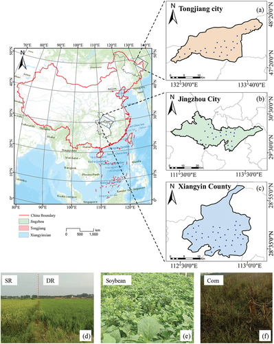
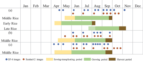
Figure 2. Rice phenology and the time of acquisition of the GF6 and Sentinel–2 images: (a) study site 1; (b) study site 2; (c) study site 3. The middle rice in the figure represents SR, and the DR contains both early rice and late rice.

2.2. Data and processing

The 2021 and 2019 Sentinel-2A/B MSI data covering three study sites with a temporal resolution of 5 days and a spatial resolution of 10–60 m were obtained from the Copernicus Data Center of the European Space Agency (ESA), including 16 images from study site 1 (T49RFN, T49RFM), 54 images from study site 2 (T49REN, T49REP, T49RFN, T49RFP, T49RGN, T49RGP), and 54 images from study site 3 (T53UMP, T53ULP, T53TMN, T53TLN, T52UGU, T52TGT). The Sentinel-2 data contain 13 bands, including visible, near-infrared and shortwave bands. The acquisition times of the Sentinel-2 images at different study sites are shown in Figure 2, and level 2A products were used. The acquired images were resampled to a spatial resolution of 20 m. The 2021 and 2019 GF-6 wide-field view (WFV) data encompassing three study sites with a revisit cycle of 4 days and a spatial resolution of 16 m were obtained from the China Resource Satellite Applications Centre (CRASAC), including 12 images from study site 1, 11 images from study site 2 and 19 images from study site 3. The GF6 data contain eight bands, including two red-edge bands that are sensitive to the chlorophyll content of plants. The details of the acquired images at different study sites are shown in Figure 2. SNAP and ENVI 5.3 software were used to preprocess the Sentinel-2 data and GF-6 data, respectively. All images were preprocessed via the following steps, radiometric calibration, atmospheric correction, orthographic correction and geometric correction.

Both GF-6 WFV and Sentinel-2 MSI images have red-edge bands that are sensitive to vegetation and crops. Previous studies (Guo and Ren 2023; X. Q. Jiang et al. 2021) have shown that red-edge vegetation indices constructed from red-edge bands and near-infrared bands, such as the normalized difference red edge (NDRE), can improve crop classification accuracies. Therefore, NDRE was chosen as the input feature for all experiments. The NDRE can be expressed as:

(1) $\mathit{NDRE}=\frac{{\mathit{\rho }}_{\mathit{NIR}}-{\rho }_{\mathit{red}-\mathit{edge}}}{{\rho }_{\mathit{NIR}}+{\rho }_{\mathit{red}-\mathit{edge}}}$(1)

where ${\rho }_{\mathit{NIR}}$ and ${\rho }_{\mathit{red}-\mathit{edge}}$ are the reflectances corresponding to the near-infrared band, and the red-edge band, respectively.

2.3. Ground truth data

The reference sample data for each study area are obtained by combining the field survey data with Google high-resolution imagery. The field survey campaigns were conducted in May and September 2021 (site 1), August 2019 (site 2), and August 2021 (site 3). During the survey, we recorded the coordinates of different land cover types using GPS at three study sites, and collected samples of various land cover types. To solve the problem that some samples were located outside or at the edges of the rice fields and some of them were too densely distributed, we combined the field survey samples with Google high-resolution images to regenerate the polygonal areas of regions of interest (ROIs), and then selected samples from the ROIs. These samples were distributed evenly throughout the entire study area, as shown in Figure 1(a)–(c). The number of sample data points obtained from the field survey and Google Earth for the different study areas is shown in Table 1.

Table 1. The number of samples for the land cover types in the three study sites.

Land cover type	Xiangyin County	Jingzhou City	Tongjiang City
Single rice	2359	2713	3100
Double rice	2157	0	0
Corn	835	891	1022
Soybean	912	1069	1117
Water	2360	2230	2500
Forest	2040	2110	1100
Grassland	0	670	460
Building	2800	2400	2380
Sum	13463	12083	11679

3. Method

3.1. An automatic rice mapping method based on an integrated time-series gradient boosting tree (Auto-ITSGBT)

An integrated time-series gradient boosted tree rice autoextraction method (Auto-ITSGBT) is proposed. In this method, the time-series curves are first split into numerous subsequences by random intervals, and interval features, including the mean, standard deviation, and linear least squares fitting slope, are extracted from each subsequence. Then, the Fourier coefficients of the time-series curves are extracted via DFT. Finally, the pipeline mechanism is used to combine, the automatic acquisition of the above features and the gradient boosting tree classification, into a unified model framework for rice mapping.

3.1.1. Interval feature extraction for time-series curves

For each time-series curve S, its data at t_i is s_i, where the data can be spectral or vegetation index data. The mean f₁(t₁,t₂), standard deviation f₂(t₁,t₂) and slope f₃(t₁,t₂) of the linear least squares fitting of s_i are extracted as the time-series interval features between t₁ and t₂, which are expressed as Eq. (2)–Eq. (4).

(2) $f_1\left(t_1,t_2\right)=\frac{\sum _{i=t_1}^{t_2}{s}_i}{t_2-t_1+1}$(2)

(3) $f_2\left(t_1,t_2\right)=\left\{\begin{array}{c}\sqrt{\frac{{\sum }_{i=t_1}^{t_2}{\left(s_i-f_1\left(t_1,t_2\right)\right)}^2}{t_2-t_1}}{t}_2>t_1\\ 0t_2=t_1\end{array}\right.$(3)

(4) $f_3\left(t_1,t_2\right)=\left\{\begin{array}{c}\frac{{\sum }_{i=t_1}^{t_2}\left(t_i-\bar{t}\right)\left(s_i-f_1\left(t_1,t_2\right)\right)}{{\sum }_{i=t_1}^{t_2}{\left(t_i-\bar{t}\right)}^2}{t}_2>t_1\\ 0t_2=t_1\end{array}\right.$(4)

where 1≤t₁≤t₂≤N; $\bar{t}=\left(t_2+t_1\right)/2$; and N represents the total number of time-series images.

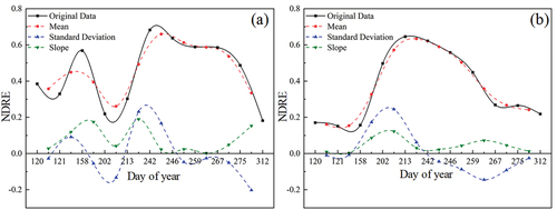
The working principle of the above interval features for capturing the key attributes of the time-series curve is shown in Figure 3. The time-series curve of f₁(t₁,t₂) can maintain a similar overall shape and value to the original time-series curve, but it is smoother and has less numerical noise than the original curve. The f₂(t₁,t₂) feature can capture the rising and falling fluctuations in the original data curve. The more severe the fluctuation is, the greater the variation caused in the f₂(t₁,t₂) curve. This feature highlights the rate of change in the original data. The f₃(t₁,t₂) feature can capture the local shape of the time-series curve, indicating whether it represents an upwards or a downwards segment. In conclusion, the interval features can be used to extract information of the original time-series curve, such as the overall values, the position of local shape change, and the magnitude of the curve variations, to obtain the key properties of the time-series curve.

Figure 3. Comparison between the original data and interval feature data of the NDRE for DR and SR. The interval features include the mean f₁(t₁,t₂), standard deviation f₂(t₁,t₂) and slope f₃(t₁,t₂). (a) is the original data and interval feature data of the NDRE for DR, while (b) is the original data and interval feature data of the NDRE for SR.

3.1.2. Integral feature extraction for time-series curves based on DFT

Each time-series curve can be expressed as an infinite series superposition of orthogonal functions, which form a Fourier series when trigonometric functions are used as basis functions. Agrawal et al. (1993) found that DFT preserves the Euclidean distance in the time or frequency domain, and the first few Fourier coefficients can indicate the principal features of the curves. Therefore, the Fourier coefficients obtained by DFT were used to represent the overall shape features of the time-series curves. For each time-series curve, s(n), consisting of N points, where n = 1, 2…, N, the t-th Fourier decomposition of s(n) can be denoted by the following equation:

(5) $\mathit{s}\left(\mathit{n}\right)=\frac{A_0}{2}+\sum _{\mathit{t}=1}^N\left[A_{t}cos\left(\frac{2\mathit{\pi tk}}{N}\right)+B_{t}sin\left(\frac{2\mathit{\pi tk}}{N}\right)\right]=\frac{A_0}{2}+\sum _{\mathit{t}=1}^N{C}_{t}sin\left(\frac{2\mathit{\pi tk}}{N}+\mathit{\phi }\right)$(5)

where

(6) $\frac{A_0}{2}=\frac{1}{N}\sum _n^N{s}_n$(6)

(7) $A_t=\frac{2}{N}\sum _n^N{s}_{n}cos\left(\frac{2\mathit{\pi tk}}{N}\right)$(7)

(8) $B_t=\frac{2}{N}\sum _n^N{s}_{n}sin\left(\frac{2\mathit{\pi tk}}{N}\right)$(8)

(9) $C_t=\sqrt{\left(A_t^2+B_t^2\right)}$(9)

(10) ${\phi }_t=arctan\left(-\frac{A_t}{B_t}\right)$(10)

In the above equations, t is the number of Fourier decompositions; N is the maximum number of decompositions; A_t, B_t and C_t represent the amplitudes; and φ_t represents the phase information.

3.1.3. Gradient boosting tree algorithm

The gradient boosting tree (GBT) (Ke et al. 2017; Konstantinov and Utkin 2021) is a type of boosting algorithm. First, a base classifier is trained using the initial training set, the misclassified samples are focused on, and the spatial distribution of the samples is adjusted. Second, the next base classifier is trained with the adjusted samples. These steps are repeated until the defined target is reached. Finally, the base classifiers are linearly combined to obtain a strong classifier. A schematic diagram of this algorithm is shown in Figure 4. Each iteration is based on the previous iteration. As the number of iterations increases, the gap between the actual and predicted values decreases. The final predicted value $\hat{y}$ of the GBT algorithm can be expressed as:

Figure 4. Schematic diagram of the GBT algorithm, where X represents the input features, and tree represents the decision tree. In this study, X refers to the interval features and Fourier coefficients of the time-series data.

(11) $\frac{3\mathit{pt}⌢}{y}={\frac{3\mathit{pt}⌢}{y}}_1+\sum _{\mathit{i}=1}^{\mathit{N}-1}{\frac{3\mathit{pt}⌢}{r}}_{\mathit{i}}$(11)

where ${\frac{3\mathit{pt}⌢}{y}}_1$ represents the predicted value of the first decision tree; ${\frac{3\mathit{pt}⌢}{r}}_{\mathit{i}}$ represents the optimal residual fit value of the i + 1th decision tree; and N is the number of decision trees.

3.2. Comparison of the Auto-ITSGBT with competing methods

To test the performance of the proposed method, we compare it with three competing methods, which are time-series random forest (TSRF), dynamic time warping (DTW) and stability weighted voting (SWV).

The TSRF (Deng et al. 2013) is a machine learning method specifically designed for time-series data. It first divides the time series into several subsequences using arbitrary time intervals and replaces the original time-series data with a collection of statistical features such as the mean, variance and slope of the subsequences. Then, these features are combined with a random forest for prediction. This algorithm was proven to be superior in time-series data classification.

The DTW (Sharma and Sundaram 2016) is a method for measuring the shape similarity of time-series curves, which enables robustness to the time shifts. To achieve this goal, the time axis can be nonlinearly “warped” to match the corresponding points between two time series.

The SWV (Shen et al. 2018) is a classification method that incorporates multiple classifiers. It combines six classifiers, including the Random Forest (RF), decision tree (DT), K nearest neighbors (KNN), support vector machine (SVM), gradient boosting tree (GBT) and BP neural network (BPNN). The weights for each classifier are determined based on their accuracy, and the final result is determined by voting among the classifiers. This method leverages the advantages of multiple classifiers, and generally outperforms methods utilizing a single classifier.

The samples in the three study areas were divided into training, validation and test sets with proportions of 40%, 40% and 20%, respectively. The role of the training data in the construction of the standard NDRE time-series curve library of land cover types is unique to the DTW method. The validation data and the test data were used to select the optimal parameters for the model and to evaluate the accuracy of the different methods.

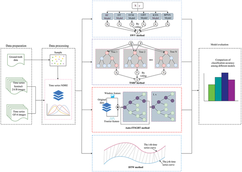
The rice mapping performances of the different methods were evaluated by a confusion matrix. The specific evaluation indices included overall accuracy (OA), user accuracy (UA), producer accuracy (PA) and the Kappa coefficient. The specific workflow diagram is shown in Figure 5.

Figure 5. The flowchart compares the effectiveness of the Auto–ITSGBT method proposed in this paper with competing methods including the TSRF method, DTW method, and SWV method for rice mapping.

4. Results

4.1. Comparison of rice mapping results between the Auto-ITSGBT method and competing methods

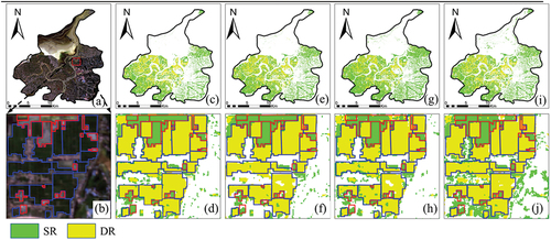
The results of the Auto-ITSGBT method and the compared methods for rice mapping at study site 1 are shown in Table 2 and Figure 6. The OA for all four methods was over 93%, indicating that the above methods, combined with time-series features, effectively achieved rice mapping. The Auto-ITSGBT method achieved OA and Kappa coefficient values of 96.45% and 0.95, respectively, and its PA and UA for both rice and nonrice crops were over 95%. Compared with the OAs of the TSRF, DTW and SWV methods, the OA of the proposed method was improved by 2% to 3%, which demonstrated the effectiveness and superiority of the proposed method for rice mapping in the mixed cropping area of single and double rice. Figure 6 shows that the Auto-ITSGBT and TSRF methods exhibited more accurate and complete results in identifying the mixed areas of single and double rice, while the results of the DTW and SWV methods confused single and double rice more often. The Auto-ITSGBT method identified more complete rice field plots with less noise than the results obtained by the other three methods.

Figure 6. Results of rice mapping based on four methods at study site 1: (a–b) the original image and the local area (GF–6 on June 7, 2021); (c–d) Auto-ITSGBT-based rice mapping result; (e–f) TSRF-based rice mapping result; (g–h) DTW-based rice mapping result; (i–j) SWV-based rice mapping result.

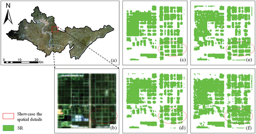
Table 2. Accuracy comparison of four rice mapping methods at study site 1.

Paddy rice map	Class	PA%	UA%	OA%	Kappa
Auto-ITSGBT	Double rice	96.19	96.31	96.45	0.95
	Single rice Non-rice	97.12 96.14	95.22 97.55
TSRF	Double rice	92.63	93.97	94.32	0.91
	Single rice Non-rice	95.25 94.98	93.27 95.44
DTW	Double rice	92.39	93.39	94.03	0.91
	Single rice Non-rice	95.13 94.50	93.38 95.05
SWV	Double rice	91.68	92.67	93.17	0.89
	Single rice Non-rice	94.88 93.05	92.34 94.23

We compared the computational efficiencies of the Auto-ITSGBT method and the three competing methods based on the time required for rice mapping in study area 1. The image size of study area 1 is 2508 × 2979, and the time series of each pixel is a superposition of 20-phase NDRE data. The computational platform used was Python 3.8.2, with an Intel core i7 9700 processor and 16 GB of RAM. The Auto-ITSGBT method took 18.43 s to infer the image of the study site when recognizing SR, DR and nonrice. DTW, TSRF and SWV took 8 h 51 min 36 s, 117.50 s, and 3 h 47 min 19 s, respectively, under the same conditions. Among them, DTW and SWV were self-programmed, and the TSRF was called pyts 0.13.0. The computational efficiency of the Auto-ITSGBT method is superior to that of the three compared methods, and the efficiency is applicable to large-scale rice mapping.

4.2. Validation of the Auto-ITSGBT-based method for rice mapping

To evaluate the robustness of the proposed method, the method was also validated at study site 2 with the similar planting pattern, and at study site 3 with different planting patterns. The results are depicted in Table 3, Figures 7 and 8. At study site 2, the OA of rice mapping using the Auto-ITSGBT was 97.13%, with a Kappa coefficient of 0.94, and the PA and UA were both greater than 96%. Compared with those of the TSRF, DTW, and SWV methods, the OA of the proposed method was 3% to 4% greater, which indicated that the proposed method was superior to the compared methods for rice mapping. At study site 3, the OA of rice mapping using the Auto-ITSGBT was 96.63%, with a Kappa coefficient of 0.93. Compared with the other methods, the OA of the proposed method was 3% to 4% greater.

Figure 7. Results of rice mapping based on four methods at study site 2: (a–b) the original image and the local area (GF–6 on August 17, 2021); (c) Auto–ITSGBT–based rice mapping result; (d) TSRF–based rice mapping result; (e) DTW–based rice mapping result; (f) SWV-based rice mapping result.

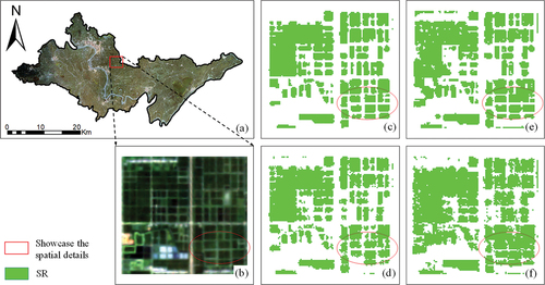
Figure 8. Results of rice mapping based on four methods at study site 3: (a–b) the original image and the local area (GF–6 on August 20, 2019); (c) Auto-ITSGBT-based rice mapping result; (d) TSRF-based rice mapping result; (e) DTW-based rice mapping result; (f) SWV-based rice mapping result.

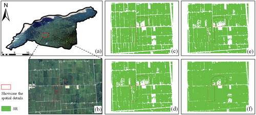
Table 3. Accuracy comparison of the four rice mapping methods at study sites 2 and 3.

Study site	Paddy rice map	Class	PA%	UA%	OA%	Kappa
Study site 2 (Jingzhou City)	Auto-ITSGBT	Rice	96.99	97.16	97.13	0.94
		Non-rice	97.28	97.12
	TSRF	Rice	93.97	94.31	94.28	0.89
		Non-rice	94.57	94.25
	DTW	Rice	93.79	93.63	93.84	0.88
		Non-rice	93.89	94.05
	SWV	Rice	92.91	93.40	93.32	0.87
		Non-rice	93.72	93.24
Study site 3 (Tongjiang City)	Auto-ITSGBT	Rice	97.34	95.57	96.63	0.93
		Non-rice	95.98	97.59
	TSRF	Rice	94.69	94.27	94.79	0.90
		Non-rice	94.88	95.25
	DTW	Rice	92.92	93.66	93.70	0.87
		Non-rice	94.40	93.74
	SWV	Rice	92.30	92.87	93.04	0.86
		Non-rice	93.70	93.18

Study sites 2 and 3, marked by red circles (Figures 7 and 8), illustrate that the Auto-ITSGBT method achieved less noise and more integrated detail performance than the other methods. The TSRF method achieves the second highest accuracy. The results of the DTW method and SWV method were noisy, and rice plot identification using these methods was incomplete (Figure 7). The red box 2 in Figure 8 shows that the rice plots extracted by the proposed method were more complete, and the contours of the rice plots were well extracted, indicating that this method could have an advantage over the other three comparative methods in identifying finely fragmented plots. This result indicates that the DTW and SWV methods were still insufficient for exploiting the local and overall shape features of time-series curves. The excessive concentration of local features in the TSRF method, and the emphasis on the distorted matching of the local shapes in the DTW method, may contribute to their misidentification problems. The SWV method was the least effective in rice identification, as it excessively misidentified nonrice crops as rice. This is likely because the SWV method does not consider the local and overall shape features of time-series curves and is unable to effectively distinguish among land covers with phenological periods similar to those of rice, resulting in the low accuracy of the final voting results.

4.4. The results of the earliest identifiable time of rice

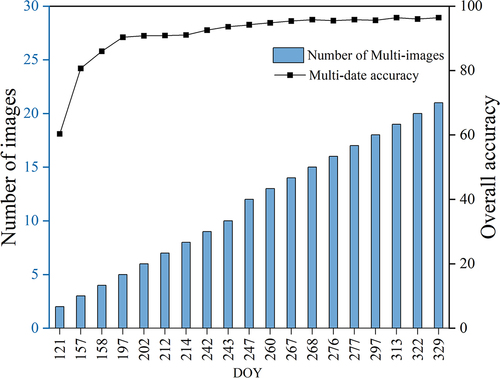
To obtain accurate rice cultivation areas as early as possible, all GF-6 and Sentinel-2 images of study site 1 were arranged in chronological order, the proposed Auto-ITSGBT method was applied to gradually reduce the number of images, and rice mapping was performed using 2 to 20 images. Figure 9 shows the curve of the overall accuracy as the number of images increases. As shown in Figure 9, the OA increases with the number of images. By mid-July (DOY of 197), a stable accuracy of over 90% is obtained, providing an accurate estimation of the area of rice cultivation before harvest.

Figure 9. Variation in OA with a gradual increase in the number of GF–6 and Sentinel-2 images based on the Auto-ITSGBT method.

5. Discussions

5.1. Analysis of the integral features extracted by DFT

Each finite-length curve can be transformed into a discrete Fourier series, and the Fourier coefficients represent the principal features of curves (Agrawal, Faloutsos, and Swami 1993). The importance of the different Fourier coefficients will be analyzed to determine the number of coefficients to be included in the rice mapping.

The GF-6-based NDRE curves of various crops were decomposed by DFT to obtain the Fourier coefficients of the frequency indices t = 0 to 5 (Table 4) and the corresponding harmonic curves (Figure 10). The amplitude of DR at t = 0 was significantly greater than that of the other three crops, indicating that the average value of the NDRE curves of DR was larger than those of SR, soybean and corn, which is possibly attributable to its long total growth period. The proportions of the amplitudes at t = 1 for SR, corn, and soybean are the largest, at 85.47%, 75.93% and 86.80%, respectively, indicating that the Fourier coefficients at t = 1 provided the most information for the time-series curves (Schäfer and Högqvist 2012). The proportions of the amplitudes at all frequency indices were significant for DR, which needed more Fourier coefficients to describe its complex curve features, as its curves had both peak-like and valley-like shapes. The cumulative proportion of amplitudes at t = 1 ~ 5 for all four crops was 100%. Therefore, in this paper, the Fourier coefficients at t = 0 ~ 5 were selected as the features for crop extraction.

Figure 10. The harmonic curves at the frequency indices t = 0 to 4 obtained from GF–6–based NDRE curves of various crops by DFT.

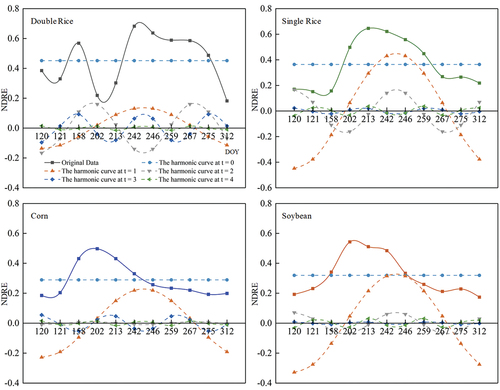
Table 4. Fourier coefficients of the GF-6-based NDRE curves for different crops at spectral coefficients t = 0 ~ 5.

cc	t	Amplitude	Phase	Amplitude		Crop type	t	Amplitude	Phase	Amplitude
				Proportion %	Cumulative proportion %					Proportion %	Cumulative proportion %
DR	0	0.45				SR	0	0.36
	1	0.15	0.47	39.89	39.89		1	0.24	1.20	85.47	85.47
	2	0.10	−0.94	19.19	59.08		2	0.08	−1.47	10.39	95.86
	3	0.11	0.47	20.34	79.42		3	0.04	0.32	1.94	97.80
	4	0.07	0.10	9.22	88.64		4	0.03	0.60	1.65	99.45
	5	0.08	−1.34	11.36	100		5	0.02	−0.15	0.55	100
Corn	0	0.29				Soybean	0	0.32
	1	0.13	−1.02	75.93	75.93		1	0.17	−1.30	86.80	86.80
	2	0.07	0.07	18.97	94.9		2	0.06	−0.64	10.68	97.48
	3	0.03	1.41	3.26	98.16		3	0.01	0.92	0.09	97.57
	4	0.02	0.43	1.45	99.61		4	0.02	−1.21	0.86	98.43
	5	0.01	−0.79	0.39	100		5	0.02	0.23	1.57	100

Figure 10 shows that the GF-6-based NDRE curves of different crops exhibit significant differences in morphological distribution features. The curves of SR and DR had both peak-like and valley-like shapes due to the transplanting period, and the curves of corn and soybean exhibited single-peak features. Therefore, considering the overall shape features of time-series curves for different land cover types can aid in their precise identification. The above analyses demonstrate that a few Fourier coefficients can represent the principal overall shape features of the curves; therefore, using Fourier coefficients to represent the integral features of the time-series curves, and as the input features for rice mapping, is reasonable and meaningful.

5.2. Application and advantage analysis of the Auto-ITSGBT method in rice mapping

Numerous studies have shown that rice mapping based on time-series remote sensing images can improve accuracy (Cai, Lin, and Zhang 2019; T. Xia et al. 2022). As discussed in Section 5.1, accounting for the overall shape of the time-series curves contributes to more accurate land cover type identification. The time-series curves of rice exhibited unique morphological features due to the transplanting period (Figure 10). However, conventional classifiers fail to consider the local or overall shape of the time-series curves, and the order in which the time-series data appear is unrelated to the classification results. The above disadvantages also make it more challenging for conventional classifiers to exclude interferences from land cover types with similar phenological and spectral features as rice. In contrast, the Auto-ITSGBT method accounts for the local shape features of time-series curves at arbitrary intervals, considers the overall shape features of different curves, and employs a pipeline mechanism that combines the automatic extraction of the above features and gradient boosting tree classification into a unified model framework. Although the growth periods of SR, soybean and corn are similar, the Auto-ITSGBT method can fully explore the overall or local differences in diverse curves, distinguish crops from similar phenological features, and improve the rice mapping accuracies. The results at three study sites show that the Auto-ITSGBT method achieves an OA 2% to 4% better than those of the DTW, TSRF and SWV methods, and the robustness in different regions is satisfactory, which indicates the effectiveness of the Auto-ITSGBT method in rice mapping, and its universality in different regions (Figures 6–8).

5.3. Analysis of the earliest identifiable time of rice

Rice mapping in practice requires obtaining a high overall accuracy and acquiring the planting area as early as possible. It requires obtaining high rice acreage accuracy by using the least number of images before harvesting. The 2nd to 20th images were selected separately for rice mapping. Both the SR and DR could be accurately identified as early as mid-July, with a consistent accuracy of over 90% (Figure 9). Accurate rice mapping can be obtained as early as 2–3 months before the middle and late rice harvest by using this method; these results align with those of Xia et al. (2022b). However, the proposed method recognizes the SR and DR, resulting in greater complexity than the work of Xia et al. (2022b), who extracted only the SR. The faster growth in the first five periods (DOY 197) was due to the transplanting period of the SR. The peak-like shape and valley-like shape begin appearing in the SR time-series curve, which is a unique phenological feature that contributes to distinguishing DR from SR. This is why satisfactory accuracies were achieved in this period. The period from DOY 202 to 242 encompassed a transplanting period of late rice, and the unique morphological features of the DR NDRE curve began to appear, contributing to the accelerated growth of the OA. The proposed method is effective in obtaining rice planting areas with high accuracy before harvest.

6. Conclusion

In this study, the Auto-ITSGBT was proposed for early and accurate acquisition of rice distribution maps using GF-6 WFV and Sentinel-2 MSI data. Compared to previous research, this method accounts for the local shape features of the time-series curves at arbitrary intervals, as well as the overall shape features of the different curves, and fully explores the information related to the phenological characteristics. The method was first tested in Hunan Province, which features a mix of single- and double-cropped rice and small-sized and fragmented rice fields. The robustness of the method was verified in the Hubei and Heilongjiang provinces, where climatic conditions, topographies or cropping patterns vary significantly. The major conclusions include the following: (1) the OA of the Auto-ITSGBT method is 2% to 4% higher than those of the DTW, TSRF and SWV methods, with an OA surpassing 95% in all validation areas. (2) Based on the Auto-ITSGBT method, with an OA of no less than 90%, a high-precision spatial distribution map for the rice can be obtained in mid-July before harvesting. The above results indicate the effectiveness and robustness of the proposed method in this paper in early and accurate rice mapping, and the method provides a reliable solution for rice mapping in different climate types.

Highlights

• Structural relationships between time-series data are crucial for accurate paddy rice mapping.

• The Auto-ITSGBT achieves accurate detection of rice mapping based on GF-6 and Sentinel-2 data.

• Auto-ITSGBT fully mines the local and integral dependencies of time-series data.

• The earliest identifiable time of accurate rice mapping in Hunan region is in mid-July.

CRediT authorship contribution statement

Xueqin Jiang: Conceptualization, Methodology, Data curation, Software, Writing – original draft, Formal analysis, Funding acquisition, Investigation. Huaqiang Du: Investigation Writing – review & editing. Song Gao: Validation, Visualization, Writing – original draft. Shenghui Fang: Conceptualization, Writing – review & editing. Yan Gong: Conceptualization, Writing – review & editing. Ning Han: Writing – review & editing.

Disclosure statement

No potential conflict of interest was reported by the author(s).

Data availability statement

The data that support the findings of the study area are available from the first author [Xueqin Jiang, [email protected]] upon reasonable request.

Supplementary Material

Supplemental data for this article can be accessed online at https://doi.org/10.1080/15481603.2024.2367807

Additional information

Funding

This work was supported by the Research Development Fund of Zhejiang A & F University (2023LFR031) and Scientific Research Fund of Zhejiang Provincial Education Department (Y202351543). Thanks to ESA and CRASAC for the free data.

References

- Agrawal, R., C. Faloutsos, and A. N. Swami. 1993. “Efficient Similarity Search in Sequence Databases.” Foundations of Data Organization and Algorithms, FODO 1993. Lecture Notes in Computer Science, Vol. 730, 69–16. Berlin, Heidelberg: Springer. https://doi.org/10.1007/3-540-57301-1_5.
- Bachelet, D. 1995. “Rice Paddy Inventory in a Few Provinces of China Using AVHRR Data.” Geocarto International 10 (1): 23–38. https://doi.org/10.1080/10106049509354476.
- Cai, Y. T., H. Lin, and M. Zhang. 2019. “Mapping Paddy Rice by the Object-Based Random Forest Method Using Time Series Sentinel-1/sentinel-2 Data.” Advances in Space Research 64 (11): 2233–2244. https://doi.org/10.1016/j.asr.2019.08.042.
- Deng, H. T., G. Runger, E. Tuv, and M. Vladimir. 2013. “A Time Series Forest for Classification and Feature Extraction.” Informing Science 239:142–153. https://doi.org/10.1016/j.ins.2013.02.030.
- Dong, J., X. Xiao, M. A. Menarguez, G. Zhang, Y. Qin, D. Thau, C. Biradar, and B. Moore III. 2016. “Mapping Paddy Rice Planting Area in Northeastern Asia with Landsat 8 Images, Phenology-Based Algorithm and Google Earth Engine.” Remote Sensing of Environment 185:142–154. https://doi.org/10.1016/j.rse.2016.02.016.
- Elliott, J., D. Deryng, C. Mueller, K. Frieler, M. Konzmann, D. Gerten, M. Glotter. 2014. “Constraints and Potentials of Future Irrigation Water Availability on Agricultural Production Under Climate Change.” Proceedings of the National Academy of Sciences 111 (9): 3239–3244. https://doi.org/10.1073/pnas.1222474110.
- Guo, Y., and H. Ren. 2023. “Remote Sensing Monitoring of Maize and Paddy Rice Planting Area Using GF-6 WFV Red Edge Features.” Computers and Electronics in Agriculture 207:107714. https://doi.org/10.1016/j.compag.2023.107714. 107714.
- Hao, P., H. Tang, Z. Chen, Q. Meng, and Y. Kang. 2020. “Early-Season Crop Type Mapping Using 30-M Reference Time Series.” Journal of Integrative Agriculture 19 (7): 1897–1911. https://doi.org/10.1016/S2095-3119(19)62812-1.
- He, Y., J. Dong, X. Liao, L. Sun, Z. Wang, N. You, Z. Li, and P. Fu. 2021. “Examining Rice Distribution and Cropping Intensity in a Mixed Single- and Double-Cropping Region in South China Using all Available Sentinel 1/2 Images.” International Journal of Applied Earth Observation and Geoinformation 101:102351. https://doi.org/10.1016/j.jag.2021.102351.
- Jiang, X. Q., S. H. Fang, X. Huang, Y. H. Liu, and L. L. Guo. 2021. “Rice Mapping and Growth Monitoring Based on Time Series GF-6 Images and Red-Edge Bands.” Remote Sensing 13 (4): 579. https://doi.org/10.3390/rs13040579.
- Jiang, X. Q., S. J. Luo, S. Gao, S. H. Fang, Y. Y. Wang, K. L. Yang, Q. Xiong, and Y. J. Li. 2022. “An Automatic Rice Mapping Method Based on Constrained Feature Matching Exploiting Sentinel-1 Data for Arbitrary Length Time Series.” International Journal of Applied Earth Observation and Geoinformation 114:12. https://doi.org/10.1016/j.jag.2022.103032.
- Jiang, R., A. Sanchez-Azofeifa, K. Laakso, Y. Xu, Z. Y. Zhou, X. W. Luo, J. H. Huang, X. Chen, and Y. Zang. 2021. “Cloud Cover Throughout all the Paddy Rice Fields in Guangdong, China: Impacts on Sentinel 2 MSI and Landsat 8 OLI Optical Observations.” Remote Sensing 13 (15): 17. https://doi.org/10.3390/rs13152961.
- Jo, H., E. Park, V. Sitokonstantinou, J. Kim, S. Lee, A. Koukos, and W. Lee. 2023. “Recurrent U-Net Based Dynamic Paddy Rice Mapping in South Korea with Enhanced Data Compatibility to Support Agricultural Decision Making.” GIScience & Remote Sensing 60 (1): 1. https://doi.org/10.1080/15481603.2023.2206539.
- Ke, G. L., Q. Meng, T. Finley, T. F. Wang, W. Chen, W. D. Ma, Q. W. Ye, and T. Y. Liu. 2017. “LightGBM: A Highly Efficient Gradient Boosting Decision Tree.” In 31st Annual Conference on Neural Information Processing Systems (NIPS). Neural Information Processing Systems (Nips), Long Beach, CA.
- Konstantinov, A. V., and L. V. Utkin. 2021. “Interpretable Machine Learning with an Ensemble of Gradient Boosting Machines.” Knowledge-Based Systems 222:16. https://doi.org/10.1016/j.knosys.2021.106993.
- Li, W., Z. Niu, R. Shang, Y. Qin, L. Wang, and H. Chen. 2020. “High-Resolution Mapping of Forest Canopy Height Using Machine Learning by Coupling ICESat-2 LiDAR with Sentinel-1, Sentinel-2 and Landsat-8 Data.” International Journal of Applied Earth Observation and Geoinformation 92:102163. https://doi.org/10.1016/j.jag.2020.102163.
- Liu, L., X. Xiao, Y. Qin, J. Wang, X. Xu, Y. Hu, and Z. Qiao. 2020. “Mapping Cropping Intensity in China Using Time Series Landsat and Sentinel-2 Images and Google Earth Engine.” Remote Sensing of Environment 239:111624. https://doi.org/10.1016/j.rse.2019.111624.
- Ni, R., J. Tian, X. Li, D. Yin, J. Li, H. Gong, J. Zhang, L. Zhu, and D. Wu. 2021. “An Enhanced Pixel-Based Phenological Feature for Accurate Paddy Rice Mapping with Sentinel-2 Imagery in Google Earth Engine.” ISPRS Journal of Photogrammetry & Remote Sensing 178 (18): 282–296. https://doi.org/10.1016/j.isprsjprs.2021.06.018.
- Oliphant, A. J., P. S. Thenkabail, P. Teluguntla, J. Xiong, M. K. Gumma, R. G. Congalton, and K. Yadav. 2019. “Mapping Cropland Extent of Southeast and Northeast Asia Using Multi-Year Time-Series Landsat 30-M Data Using a Random Forest Classifier on the Google Earth Engine Cloud.” International Journal of Applied Earth Observation and Geoinformation 81:110–124. https://doi.org/10.1016/j.jag.2018.11.014.
- Salmon, J. M., M. A. Friedl, S. Frolking, D. Wisser, and E. M. Douglas. 2015. “Global Rain-Fed, Irrigated, and Paddy Croplands: A New High Resolution Map Derived from Remote Sensing, Crop Inventories and Climate Data.” International Journal of Applied Earth Observation and Geoinformation 38:321–334. https://doi.org/10.1016/j.jag.2015.01.014.
- Schäfer, P., and M. Högqvist. 2012. “SFA: A Symbolic Fourier Approximation and Index for Similarity Search in High Dimensional Datasets.” In International Conference on Extending Database Technology, Berlin, Germany, 516–527.
- Sharma, A., and S. Sundaram. 2016. “An Enhanced Contextual DTW Based System for Online Signature Verification Using Vector Quantization.” Pattern Recognition Letters 84 (15): 22–28. https://doi.org/10.1016/j.patrec.2016.07.015.
- Shen, H. F., Y. H. Lin, Q. J. Tian, K. J. Xu, and J. N. Jiao. 2018. “A Comparison of Multiple Classifier Combinations Using Different Voting-Weights for Remote Sensing Image Classification.” International Journal of Remote Sensing 39:3705–3722. https://doi.org/10.1080/01431161.2018.1446566.
- Thenkabail, P. S., V. Dheeravath, C. M. Biradar, O. R. P. Gangalakunta, P. Noojipady, C. Gurappa, M. Velpuri, M. Gumma, and Y. Li. 2009. “Irrigated Area Maps and Statistics of India Using Remote Sensing and National Statistics.” Remote Sensing 1 (2): 50–67. https://doi.org/10.3390/rs1020050.
- Thorp, K. R., and D. Drajat. 2021. “Deep Machine Learning with Sentinel Satellite Data to Map Paddy Rice Production Stages Across West Java, Indonesia.” Remote Sensing of Environment 265:13. https://doi.org/10.1016/j.rse.2021.112679.
- Wang, L., H. Ma, J. Li, Y. Gao, L. Fan, Z. Yang, Y. Yang, and C. Wang. 2022. “An Automated Extraction of Small- and Middle-Sized Rice Fields Under Complex Terrain Based on SAR Time Series: A Case Study of Chongqing.” Computers and Electronics in Agriculture 200:107232. https://doi.org/10.1016/j.compag.2022.107232.
- Wei, J., Y. Cui, W. Luo, and Y. Luo. 2022. “Mapping Paddy Rice Distribution and Cropping Intensity in China from 2014 to 2019 with Landsat Images, Effective Flood Signals, and Google Earth Engine.” Remote Sensing 14 (3): 759. https://doi.org/10.3390/rs14030759.
- Weiss, M., F. Jacob, and G. Duveiller. 2020. “Remote Sensing for Agricultural Applications: A Meta-Review.” Remote Sensing of Environment 236:19. https://doi.org/10.1016/j.rse.2019.111402.
- Xia, T., Z. He, Z. W. Cai, C. Wang, W. J. Wang, J. Y. Wang, Q. Hu, and Q. Song. 2022. “Exploring the Potential of Chinese GF-6 Images for Crop Mapping in Regions with Complex Agricultural Landscapes.” International Journal of Applied Earth Observation and Geoinformation 107:12. https://doi.org/10.1016/j.jag.2022.102702. 2022.102702.
- Xia, L., F. Zhao, J. Chen, L. Yu, M. Lu, Q. Y. Yu, S. F. Liang. 2022. “A Full Resolution Deep Learning Network for Paddy Rice Mapping Using Landsat Data.” ISPRS Journal of Photogrammetry and Remote Sensing 194:91–107. https://doi.org/10.1016/j.isprsjprs.2022.10.005.
- Yang, H., B. Pan, W. Wu, and J. Tai. 2018. “Field-Based Rice Classification in Wuhua County Through Integration of Multi-Temporal Sentinel-1A and Landsat-8 OLI Data.” International Journal of Applied Earth Observation and Geoinformation 69:226–236. https://doi.org/10.1016/j.jag.2018.02.019.
- Yeom, J., S. Jeong, R. C. Deo, and J. Ko. 2021. “Mapping Rice Area and Yield in Northeastern Asia by Incorporating a Crop Model with Dense Vegetation Index Profiles from a Geostationary Satellite.” GIScience & Remote Sensing 58 (1): 1–27. https://doi.org/10.1080/15481603.2020.1853352.
- Zhang, X., F. Qiu, and F. Qin. 2019. “Identification and Mapping of Winter Wheat by Integrating Temporal Change Information and Kullback–Leibler Divergence.” International Journal of Applied Earth Observation and Geoinformation 76:26–39. https://doi.org/10.1016/j.jag.2018.11.002.
- Zhang, C., H. Zhang, and S. Tian. 2023. “Phenology-Assisted Supervised Paddy Rice Mapping with the Landsat Imagery on Google Earth Engine: Experiments in Heilongjiang Province of China from 1990 to 2020.” Computers and Electronics in Agriculture 212:108105. https://doi.org/10.1016/j.compag.2023.108105.
- Zhu, L., X. Liu, L. Wu, M. Liu, Y. Lin, Y. Meng, L. Ye, Q. Zhang, and Y. Li. 2021. “Detection of Paddy Rice Cropping Systems in Southern China with Time Series Landsat Images and Phenology-Based Algorithms.” GIScience & Remote Sensing 58 (5): 733–755. https://doi.org/10.1080/15481603.2021.1943214.
- Zupanc, A. 2017. “Improving Cloud Detection with Machine Learning.” https://medium.com/sentinel-hub/improving-cloud-detection-with-machine-learning-c09dc5d7cf13.