Mapping recent timber harvest activity in a temperate forest using single date airborne LiDAR surveys and machine learning: lessons for conservation planning

ABSTRACT

Effective planning for natural resource management and wildlife conservation requires detailed information on vegetation structure at landscape scales and how structure is influenced by land-use practices. In many forested landscapes, the largest impacts of land use on forest structure are driven by forest management activities, which can include invasive species control, prescribed fire, partial harvests (e.g. shelterwood harvests) or overstory removals and clearcuts. Active timber management is often used to achieve forest conservation objectives, but to be used effectively, managers require knowledge of harvest frequency and extent in adjacent forests and at landscape scales. In this paper, we develop a timber harvest mapping workflow using machine learning (XGBoost algorithm) and single campaign airborne light detection and ranging (LiDAR) surveys for the state of Pennsylvania, USA. We show that harvest type (shelterwood and overstory removals) can be mapped at high accuracy (overall accuracy = 94.9%), including broad age classes defined by the number of years since harvest. Errors of omission (false negatives) were lowest for recent (<10 yr old) overstory removal harvests (1.5%) and highest for older (10–18 yr old) shelterwood harvests (34.9%), which is consistent with the expectation that older, partial timber harvests are more difficult to distinguish from untreated forests than are recent harvests. Errors of commission (false positives) were low (<6.0%) for all timber harvest types and ages. Analysis of model results across both public and private lands in three highly forested conservation regions of Pennsylvania (the Poconos, PA Wilds, and Laurel Highlands) revealed a propensity for young overstory removals along forest edges, suggesting edge effects from inaccuracies in the underlying forest mask and mixed pixels contribute to errors of commission. Acknowledging this, overstory removal and shelterwood harvests were roughly equally common across public and private lands when expressed as a fraction of all interior forests (forests >30 m from an edge). The expectation that these harvest treatments would be rarer in private forests was not supported by the model results, which is likely due to the model’s inability to distinguish between alternative natural processes (weather damage, wildfire, pathogens, etc.) and forest treatment types (high-grading and firewood collection) that result in similar forest structures to the trained classes in the XGBoost model. This study provides a framework and validation for combining approachable machine-learning techniques with large-campaign LiDAR to accurately predict forest structure with application to a host of forestry, natural resource, and conservation-related problems. Future efforts that refine the model’s ability to better distinguish between more complex harvest classes and natural processes would be valuable.

KEYWORDS:

• Forest structure
• XGBoost
• overstory removal
• shelterwood
• private land
• public land

1. Introduction

It is increasingly apparent that natural resource management and the conservation of biological diversity requires strategies with landscape perspectives (Parent and Hernández 2021). In forest systems, this can involve indicating progress toward management goals using metrics related to forest area, stand age-class distribution, forest patch size and connectivity, and/or diversity in forest structure and community type (Baskent and Keles 2005; Boutin and Hebert 2002). Diversity in forest structure is important for wildlife conservation because species vary in habitat preferences and some individual species even vary in their own needs during different lifecycle stages (Fiss et al. 2020). Forest structure is also important to foresters who, in part, use structural cues to determine where and when to implement various management practices (Achim et al. 2021; Loftis 1990). Therefore, quantifying forest structural components and developing understanding of how the diversity and configuration of these components informs conservation planning is an important challenge when managing for biodiverse ecosystems (Schwenk and Donovan 2011). Methods quantifying forest disturbance patterns and anthropogenic processes affecting forest and landscape structure are thus key to the development of ecological indicators (Pressey et al. 2007). This is particularly true where active forest management is implemented with the intention of sustainably provisioning wood fiber and creating habitat for at-risk species. For example, in the Appalachian Mountains of the USA, multiple public and private conservation groups are currently focused on better meeting the habitat needs of diverse forest bird communities by increasing forest structural diversity at landscape scales through active forest management that includes sustainable timber harvest practices (Litvaitis et al. 2021; McNeil et al. 2020; U.S. Fish & Wildlife Service 2006).

Geographical data that track forest and landscape structure, including measures of progress toward landscape-scale stand diversity goals, have typically been provided either through management records or time-series of remotely sensed images (e.g. Landsat (Hermosilla et al. 2018; Wulder et al. 2004; Zhu et al. 2020)). Methods that can consistently detect and map forest harvest activity across private-public land boundaries are particularly valuable considering the large area of private land holdings and their importance to timber production and conservation planning, especially in the eastern United States (Lutter et al. 2019; North American Bird Conservation Initiative, U.S. Committee 2013). Across landscapes composed of private and public landholders, land management records are rarely consistent and sufficient to provide reliable insight about regional trends in land management and landscape structure that are needed to develop effective long-term conservation strategies. To this end, remotely sensed data have played an important role in providing both spatial and temporal information about landscape structure across a broad range of scales (Gao et al. 2020; Wulder et al. 2004). Multitemporal optical data have been the most widely used remote sensing platform because they directly track changes in forest reflectance, easily detecting full canopy removals (Hansen et al. 2013; Jarron et al. 2016; Stahl et al. 2023). Despite issues with resolution, clouds, phenology, and changes in sensors, multispectral optical imagery has provided some of the most important and widely used data on forest cover and landscape configuration of forests (Banskota et al. 2014; Pasquarella et al. 2016; Senf et al. 2017; Tortini et al. 2019; White et al. 2017). Despite these successes, optical data do not directly quantify forest structure and instead rely on changes in the relative cover of photosynthetic vegetation (e.g. green leaves) and non-photosynthetic vegetation (e.g. slash and plant litter) to indicate forest harvests (Sabol et al. 2002). Disturbance processes can vary greatly in the degree of change in these parameters (e.g. consider the effect of storm damage, pathogens, and drought relative to that of timber harvests). Furthermore, time series of optical data are only capable of detecting change over the observation period (Sanchez-Lopez, Boschetti, and Hudak 2019). Therefore, when the goal of mapping is to classify forests structurally, time series of optical data do not generally provide the needed thematic resolution, frustrating those wishing to plan and implement conservation action at landscape scales.

Airborne Light-detection and Ranging (LiDAR) provides a solution to incorporate forest structure into conservation planning (Bergen et al. 2009; Coops et al. 2016; Farrell et al. 2013; Goetz et al. 2010). Airborne LiDAR permits direct observations of forest structure, often at a fine spatial grain (<10-m pixels), yet presents new challenges due to its airborne nature, sparse temporal coverage, sensitivity to point return density and canopy condition, among other issues (Brubaker et al. 2014; Dubayah and Drake 2000). In particular, due to the expense, multitemporal airborne LiDAR data are rarely collected at time intervals necessary to directly observe active management (i.e. using before and after surveys). Therefore, active forest management and the age of past harvests must be retrieved from the structural information provided in a single survey, as has been demonstrated previously (Fedrigo et al. 2018; Maltamo et al. 2020; Racine et al. 2013). Given spatial and temporal information on past harvests, airborne LiDAR has the potential to be leveraged in a machine learning framework to predict harvest type and age across broad regions. As airborne LiDAR has improved in quality and coverage, this potential has increased (Coops et al. 2021), and may increasingly complement or even surpass the capabilities of other modeling and interpolation approaches (Hansen et al. 2014; Matasci et al. 2018; O’Neil-Dunne, MacFaden, and Royar 2014).

Overall, this survey of the literature suggests that indicating progress toward conservation goals related to the creation of early successional forest habitat requires spatial data with (1) higher spatial resolution than that afforded by medium resolution optical sensors and (2) increased thematic information related to forest structure resulting from disturbances, including from timber harvest. Therefore, the specific objective of this paper was to demonstrate the capability of single-date airborne LiDAR and machine learning for mapping classes of forest structure associated with timber harvest practices across a large spatial extent. Meeting this objective required addressing common issues encountered when working with airborne LiDAR surveys that span large areas. Airborne LiDAR data were used in combination with spatio-temporal records of past forest harvests in an application of the machine learning algorithm XGBoost to model timber harvest types and ages across most of Pennsylvania, USA, where sustainable forest management and habitat-based conservation increasingly depends on knowledge of forest structure at landscape scales, including the influence of past forest management (McNeil et al. 2020). We demonstrate that the resulting classification map can adequately summarize forest structure, namely the influence of timber harvest type and age, across private and public lands in Pennsylvania for three focal conservation regions.

2. Data and methods

2.1. Study area

Pennsylvania (PA) is 59% forested, amounting to ~16.7 million acres (~70,000 km²) of primarily Northern Hardwood and Mixed-Oak forest types (Barrett 1962). These forests contribute significantly to local and statewide economies with forest-related sectors employing over 65,000 individuals and contributing about $37 billion toward the state’s annual economy (PA-DCNR 2020). Additionally, Pennsylvania’s forests host diverse wildlife communities including many rare, threatened, and endangered species. Effectively managing these forests for both timber resources and biodiversity is complicated by numerous threats that include conversion to non-forest land uses, unsustainable timber harvests, invasive species, excessive browsing by white-tailed deer (Odocoileus virginianus), forest pests (e.g. Lymantria dispar), fire suppression, and diseases (Dey 2014). Even if these threats were mitigated, the homogeneous age structure that dominates eastern forests poses a significant challenge for meeting forestry and wildlife conservation objectives (Dey 2014; Greenberg et al. 2011; King and Schlossberg 2014). Indeed, historically important processes that would diversify forest structure through disturbance are now largely absent on the landscape (e.g. elk [Cervus canadensis] and bison [Bison bison] foraging, beaver [Castor canadensis] flooding, wildfire) (Shifley et al. 2014). Subsequently, populations of forest wildlife that rely upon ecological disturbance to meet at least some portion of their habitat needs such as the golden-winged warbler (Vermivora chrysoptera; requiring early successional forest (Fiss et al. 2020)) and cerulean warbler (Setophaga cerulea; requiring late seral forest conditions (Wood et al. 2013) and frequent canopy gaps (Boves et al. 2013)), have declined at some of the steepest rates relative to other North American songbird species (Sauer et al. 2013). The implementation of management actions aimed at improving landscape-scale structural diversity of eastern forests is a conservation priority motivated by research findings that describe its importance to ensuring long-term availability of quality timber resources (Dey 2014; Shifley et al. 2014) and recovering populations of many wildlife species (Fiss et al. 2020; King et al. 2006; Raybuck et al. 2019). As such, natural resource agencies and conservation groups have initiated ambitious efforts to use active forest management to mimic the disturbance regimes that historically created and maintained diverse forest structure across landscapes (McNeil et al. 2020; Thom and Keeton 2020).

There is wide agreement that active forest management can make important contributions to wildlife conservation through well-planned sustainable forestry practices (Litvaitis et al. 2021; Sallabanks and Arnett 2005). Central to realizing this contribution is the development of methods for mapping specific forest structure types related to management activities, and using these maps to understand progress toward landscape-level habitat goals over defined conservation regions, including both public and private lands (Dickinson, Zenner, and Miller 2014). In Pennsylvania, public agencies and their conservation partners are attempting to increase landscape structural diversity across public forests, as well as providing technical and financial assistance to private landowners to improve their forests’ health, future economic and recreational opportunities, and value as wildlife habitat (Litvaitis et al. 2021; McNeil et al. 2017). Central to this work are three regionally important conservation areas (Poconos, PA Wilds, and Laurel Highlands) (Figure 1A), that contain most of the remaining large tracts of forest within the state. Sustainable timber harvests (shelterwood and overstory removal) and other forest stand improvement practices are implemented on public and private lands within these regions with the main objective of sustainably provisioning wood fiber and enhancing forest resilience. However, it is also well understood that regenerating timber harvests provide much needed habitat for several conservation priority species in these regions (Boves et al. 2013; McNeil et al. 2018), and that disturbance intensity and time since harvest influences avian communities (Twedt 2020). Thus, having a reliable method to identify and quantify the extent and types of active forest management implemented within the PA Wilds, Laurel Highlands, and Poconos conservation areas, regardless of ownership domain, has several benefits. These include more accurate tracking of progress toward wildlife habitat goals, identification of areas still in need of management, and pinpointing opportunities to build synergy between public and private forests.

Figure 1. Maps of important features of Pennsylvania, USA. (A) Public forests (green) and areas of interest for conservation (purple), (B) LiDAR delivery areas described in Table 1, (C) airborne LiDAR survey dates, and (D) Google Eath Engine Dynamic World land cover (Brown et al. 2022).

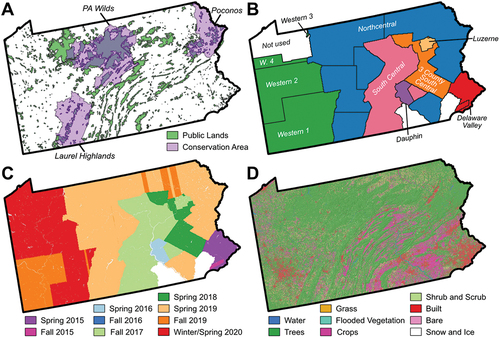
Table 1. Relevant technical and data acquisition specifics of airborne LiDAR used in this work.

Delivery Area (Quality Level) (Study Area)	Scanner (Field of View)	Swath Width (m)	Line Spacing (m)	Observed Mean Ground and Vegetation Point Densities (pts m^−2)	Collection Date Range
PA Western PA 4 2019 (QL2)(1,951 km^2)	Riegl VQ1560i (58.5°) Optech GalaxyPrime (40°)	2576 1775.16	2061 1420.13	G − 2.68 V − 1.75	11/18/19 to 5/2/20
PA Western PA 3 2019 (QL1)(70 km^2)	Optech GalaxyPrime (27°)	563	467.92	G − 8.92 V − 22.33	3/13/20 to 3/14/20
PA Western PA 2 2019 (QL2)(12,652 km^2)	Riegl VQ1560i (58.5°)	2576	2061	G − 3.71 V − 3.19	11/25/19 to 3/22/20
PA Western PA 1 2019 (QL2)(16,010 km^2)	Riegl VQ1560i (58.5°)	2576	2061	G − 3.64 V − 3.54	11/18/19 to 3/9/20
PA Northcentral B(1–5) 2019 (QL2)(47,694 km^2)	Riegl VQ1560i (58.5°) Optech Galaxy Prime (40°) Leica ALS80 (40°)	2458 1147 1265	1721 803 886	G − 3.22 V − 4.35	3/20/19 to 11/23/19
PA South Central B(1–2) 2017 (QL2)(17,916 km^2)	Leica ALS70 (36°) Leica ALS80 (34°) Riegl LMS-Q1560 (58°)	1300 1223 2129	769 688 1490	G − 2.64 V − 1.79	11/21/17 to 12/21/17
PA 3 County South Central 2018 (QL2)(7,523 km^2)	Leica ALS70 (36°)	1300	1053	G − 2.21 V − 1.63	12/2/17 to 4/13/18
PA Dauphin 2016 (QL2)(1,636 km^2)	Leica ALS70 (40°)	1510.48 1528.67	1018.43 1351.74	G − 1.71 V − 1.06	3/24/16 to 3/26/16
^aPA Luzerne County 2018 (QL1)(1,041 km^2)	Leica ALS80 (20°)	Variable	Variable	G − 3.89 V − 17.21	11/23/17 to 12/8/17
^bDE Delaware Valley HD 2015 (QL2)(4041 km^2)	Leica (28° to 40°)	792.86 to 1026.75	514.76 to 793.92	G − 1.79 V − 1.36	4/12/15 to 11/25/15

^aExplicit values were not reported for swath width and line spacing.^bParameter value ranges are reported due to variability across the region. No specific Leica lidar scanner model was reported for the Delaware Valley dataset.

2.2. Data processing

2.2.1. Airborne LiDAR surveys

We designed and implemented a workflow for mapping forest harvest types that leveraged airborne LiDAR data for most of the state of Pennsylvania. This work made synergistic use of airborne LiDAR surveys spanning a wide range of relevant collection parameters (Table 1) that resulted in a single survey occurrence for each parcel of land across the state (e.g. a given patch of earth was only imaged one time during the LiDAR campaign), except for minor overlap along adjacent flightline edges (Figure 1). Approximately three-quarters of the data used in this project were collected during 2018–2020 in five large delivery areas. The remainder of the study region was surveyed between 2015 and 2017 in five additional, smaller delivery areas. All surveys were quality level-2 or better with point counts sufficient for high-resolution digital elevation mapping. Methods for using such data to produce canopy height models are established (Dubayah and Drake 2000). However, within each delivery area, flightlines were flown over several months and with a range of survey parameters and equipment, which imposed a variety of challenges in data processing. Point densities depended on many factors, but flightline overlap doubled mean point densities in those regions. In some locations, adjacent flightlines were flown months apart. While all data were intended to be collected during leaf-off conditions, in some cases weather and other considerations forced operators to collect data into mid-to-late spring or mid fall, when leaf-out may have already begun to occur or abscission was not yet complete, respectively. Data acquisition during periods of more abundant leaf-on conditions may increase the number of canopy returns while decreasing the number of ground returns, resulting in data irregularities particularly apparent as “striping” at the boundaries of flightlines with differing data collection parameters.

LiDAR flightlines in each collection area were downloaded through the USGS 3DEP LidarExplorer website (https://apps.nationalmap.gov/lidar-explorer/.) and delivered as tiles, each 1–2.25 km² in area (Table 1). Tiles were processed individually into 10 × 10 m spatial resolution pixels for the calculation of metrics of forest structure (Table 2) using the lidR package in R (Roussel et al. 2020). For each tile, LiDAR returns in class 1 (processed but unclassified) and 2 (ground returns) were retained for analysis. Returns classified as overlap, duplicates, or withheld were removed, which reduced striping in the resulting LiDAR metrics. LiDAR returns were normalized for height using a triangulated irregular network (TIN) algorithm to construct the digital terrain model from ground returns. In total 81,793 tiles were processed covering most of Pennsylvania and resulting in 1,121,906,452 total 10 × 10 m pixels with calculated metrics.

Table 2. Descriptions of all LiDAR metrics considered for use in the predictive model.

Metric Name	Metric Description	Used in Final Model?
Standard Voxels V2 to V50	The percent of LiDAR returns in the 2 m vertical bin below XX, calculated every 2 m from ground to 50 meters height (25 total)	Yes
Special Voxels Perc_X2_to_X1	The percent of total returns between X2 and X1 meters height, calculated for 5 to 1 m, 5 to 2m, and 2 to 1m	Perc_2m_to_1m
Special First Return Voxels Perc_First_X2_to_X1	The percent of first returns between X2 and X1 meters height, calculated for 5 to 1 m, 5 to 2m, and 2 to 1m	Yes
FirstBelowXm	The percent of first returns below X meters, calculated for 1, 2, and 5 m	No
BelowXm	The percent of total returns below X meters, calculated for 1 m and 5 m	No
p5, p10, p25, p50, p75, p90, p95, p99	Height in meters below which XX percentage of LiDAR returns are found	p75, p90, p95, p99
IQR	Interquartile height range in meters	Yes
Top Rugosity	The standard deviation of the height of first returns	Yes
MOCH	Mean outer canopy height derived from the mean height of the first returns	No
M_STD30m	Standard deviation of canopy height from a 30 x 30 m moving window, calculated for p95, p99, and MOCH metrics	p95_STD30m, p99_STD30m
M_STD50m	Standard deviation of canopy height from a 50 x 50 m moving window, calculated for p95, p99, and MOCH metrics	p95_STD50m, p99_STD50m
Elevation, Slope, and Aspect	Topographic metrics derived from the 10 m NED digital elevation model (3x3 pixel mean)	Yes

Metrics were excluded from the machine learning model for a variety of reasons discussed in section 2.2.2.

2.2.2. LiDAR forest metrics

Normalized LiDAR point clouds can be distilled into a suite of metrics that quantify structural attributes of forests, including height, structural heterogeneity, canopy cover, and arrangement (Hardiman et al. 2018). All metrics selected in this study have been discussed previously in the literature and used in a wide variety of applications (Table 2) (Atkins et al. 2018; Hardiman et al. 2018; LaRue et al. 2022; McNeil et al. 2023). Our workflow began by calculating the point return density in voxels that were 2 m in the vertical dimension and 10 × 10 m in the horizontal. Point return density is typically calculated as the number of returns within the voxel divided by the sum of all returns in each column of voxels. Voxel point return densities were calculated in 2-m increments from 0 to 50 m and were expected to represent most of the variation in vegetation structure (Ciuti et al. 2018). In addition, metrics that were hypothesized to be more important for detecting vegetation structural differences in recent harvests were also included, such as those sensitive to the presence of shorter vegetation (e.g. <5 m). Unfortunately, return density in this range is highly dependent on upper canopy density and LiDAR point density (LaRue et al. 2022). Conversely, metrics that were sensitive to the upper 25% of the canopy volume were least sensitive to variations in LiDAR parameters and collection date variability. However, variation in upper canopy structure among adjacent 10 × 10 m grid cells might be indicative of small forest gaps and small (selective) harvests. Therefore, we included as metrics the standard deviation (i.e. rugosity) of metrics related to canopy height, calculated at 30 m (3 × 3 pixels) and 50 m (5 × 5 pixels) spatial resolutions.

We evaluated each LiDAR metric for potential artifacts and for the quality and consistency across delivery areas. Metrics with considerable striping were removed from the analysis (indicated in Table 2). Metrics sensitive to return densities below 5 m were particularly sensitive to flight-line striping effects. However, since metrics sensitive to short vegetation were of particular interest for mapping recent forest harvest types, we retained return density layers from voxels <6 m and return densities in the 1–2 m range despite evidence of minor striping. We found that striping was most pronounced in metrics that included data near the ground (e.g. percent of all or first returns below 1 m, 2 m, 5 m, etc.), but was less pronounced in metrics that only included data above 1 m (e.g. percent of returns between 1 and 2 m or any of the voxel density metrics above 1 m). We also found that some delivery areas contained more striping than others with the most problematic being a large area of the Western PA 4 delivery area, some of which was collected in early May 2020 after leaf-out had begun. Because we suspected that tree flowering and leaf development might have impacted these data, they were removed from the analysis. Two small delivery areas in southeastern PA were also excluded because the most recent LiDAR survey was in 2015 and the area is mostly agricultural or developed land.

2.2.3. Elevation and land cover data

LiDAR data analysis was supplemented with additional spatial data. These included a 10-m Digital Elevation Model (DEM) acquired from the National Elevation Dataset (Arundel et al. 2018). From the DEM, we calculated topographic slope and aspect using a 3 × 3 pixel window. These topographic indices were used alongside LiDAR metrics in the modeling work described below. To mask agricultural and urban lands we used the Dynamic World data set from Google Earth Engine (Figure 1D) (Brown et al. 2022). From the nine land cover classes represented in the Dynamic World data set, we selected (1) Trees and (2) Shrub and Scrub to represent the forest areas central to our modeling work. If only the Forest class was used, many areas of recent timber harvests (especially overstory removals) would have been masked out as Dynamic World frequently classifies them as Shrub and Scrub. The resulting Forest and Shrub and Scrub mask was used to remove non-forest from regional statistics reported in this paper and for display purposes when viewing map results. Additional polygon data was also acquired from government websites that helped conceptualize landscape variation in the extent of forest harvest, such as public land ownership layers (State Forests, State Game Lands, and State Parks) and polygons for three focal watershed-delineated conservation regions in Pennsylvania: the Poconos, PA Wilds, and the Laurel Highlands (Figure 1A).

2.2.4. Timber harvest data

Timber harvest data used to train and test the predictive model consisted of known areas of recent forest management, including overstory removal and shelterwood harvests (Figures 2, 3). Each instance of forest management was recorded as a polygon digitized by the PA Bureau of Forestry staff and included (1) a broad characterization of the management type, and (2) the year of implementation. These data covered all state forest lands, amounting to 727 km² of recently (<25 years old) harvested land out of a total of 8974 km² of state-owned forest land. While extensive, state-owned forest land in PA represents only approximately 13% of the total forested area in the state. The extent of the documented harvests adequately filled the spatial extent of state forest land. To ensure consistent training and test data and avoid irregular vegetation structure found at the edges of forest harvests, we applied a 30 m interior buffer to all polygons of timber management treatment boundaries. We sampled all the LiDAR metrics from all areas identified as overstory removal harvest (“removal”) or shelterwood harvest (“shelterwood”) in the PA Bureau of Forestry records. The resulting data were assembled into a table with one row for each 10 × 10 m grid cell and columns for harvest type, year of harvest, and each of the LiDAR metrics. To this table we added a column for LiDAR survey year. Harvest age was calculated as the difference between the LiDAR survey year and the year of harvest. Areas outside of any designated harvest, but within state forest lands, were assembled into an “untreated” class. These areas covered approximately 81 million 10 × 10-m pixels (8100 km²) and, after verifying that no bias was introduced into the metrics, were systematically decimated to ~2 million 10 × 10-m pixels (200 km²) to reduce computational overhead associated with training the model as well as to reduce class imbalance. The final table used included 5,524,538 rows, which were randomly split 70:30 into training and testing datasets.

Figure 2. Airborne LiDAR tiles with point return height normalized to the ground surface depicting the four different timber harvest types and ages that the XGBoost model was trained to identify. (A) Two typical overstory removal plots (2-year old and 11-year old) along with intact mature forest (untreated class) (from −77.578°W, 41.653°N). Notice the ingrowth of the understory in the older overstory removal compared to the more recent plot. (B) Two 7-year old shelterwood harvest plots showing the systematic canopy gaps typical of such harvests (from −77.929°W, 40.968°N). (C) A rare 14-year old shelterwood harvest still displaying some of the same gap structure as shown in (B) (from −77.956°W, 41.291°N).

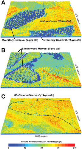
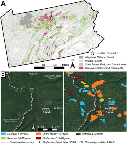
Figure 3. (A) state timber harvest data used for training and testing the XGBoost model (magenta) with a zoomed in example in (B). The speckled white areas in (B) are the decimated samples of the “untreated” forest class and the stars indicate two examples of locations where timber harvest postdated LiDAR data collection and were not used (colorless patches). Private forests shown in (A) were derived from the Dynamic World dataset (Brown et al. 2022).

Each LiDAR metric was summarized by harvest type and harvest age in 5-year increments. Harvests that were recorded as occurring in the same year as the LiDAR survey (i.e. harvest age = 0) were discarded as we did not know the specific time of year of harvest. We evaluated the apparent sensitivity of each metric to harvest age and type using violin plots (e.g. Figure 4). Decisions to retain or exclude a metric from the machine learning modeling work (given apparent striping or other data artifacts) were made, in part, based on information gathered from these violin plots. For example, the percent of all returns between 1 and 5 m did not vary strongly with harvest age, supporting the justification to remove it from the modeling workflow. We also noted that violin plots of metrics for harvests aged 10–14 years and 15–20 years were often very similar. Because there were no shelterwood harvest older than 18 years, we removed both harvest types older than 18 years. Ultimately, we formed two classes for each harvest type: 1–9 years and 10–18 years.

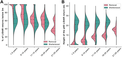
Figure 4. Violin plots showing the dependence of forest structure on forest management type and harvest age. Shown are two metrics of forest structure: (A) the percent of LiDAR returns <2m from the ground (V2), and (B) the height of the 95-th percentile return (p95). Note that the training data contains no shelterwood older than 18 years. Hashes inside the violin plots denote the inter-quartile range and median for each distribution.

2.3. XGBoost machine learning algorithm

XGBoost is a relatively recent ensemble machine learning method that has shown great promise in efficiently and accurately solving both classification and regression problems with tabular data (Chen and Guestrin 2016). XGBoost builds on the gradient boosting framework by optimizing both the efficiency of the algorithms (via parallelization) and implementing regularization, which helps to reduce overfitting. In addition, XGBoost, like other gradient boosting and decision tree algorithms, is immune to issues of multi-collinearity permitting the inclusion of diverse feature sets without a priori exclusion. The utility of the XGBoost algorithm has only recently begun to be explored in forestry studies using LiDAR, including but not limited to identifying forest stands conducive to commercial thinning (Frank et al. 2019), assessing forest attrition due to wind (Moore and Lin 2019), and predicting forest inventory and structure (Corte et al. 2020; Yu et al. 2021). We used the Python package implementation of the XGBoost library on a training dataset comprising 3,867,176 10 × 10 m pixels of 39 LiDAR-based metrics of forest structure and 3 topographic metrics. We reserved an additional 1,657,361 pixels for testing (see next section). Given the large size of the training dataset, a limited number of key hyperparameters were tuned using a standard grid search to produce the optimal model (Table 3), while all other parameters were left at their default values in XGBoost. Ideally, a large range of parameter spaces would be tuned regardless of the computational expense. However, exhaustive parameter tuning often results in very marginal increases in accuracy (1–2%) at the cost of excessive computational resources and time. Additionally, a standard train-test-split was favored over a cross validation (CV) approach, due to the computational cost associated with such a high number of records. Despite this, the standard train-test-split technique, when used on a sufficiently large dataset, does not suffer from the issue of high model variance that makes the CV technique superior for use on smaller datasets. Using the test data, optimal model accuracies were also calculated for checkerboard (5 × 5 km windows), balanced class, and unbalanced class model inputs to assess their effect on the model. Balanced and unbalanced classes had similar overall accuracies (84.0% and 90.3%, respectively) with the overall accuracy of the checkerboard implementation lower at ~73%. This discrepancy is believed to result from the spatial irregularity and heterogeneous class distribution of the training dataset. The optimal model using the unbalanced classes as input was selected to maximize overall accuracy while prioritizing the most computationally efficient hyperparameter combination (e.g. smallest number of trees and tree depth as possible). Specifically, hyperparameter values were chosen where overall accuracy values became invariant or commonly recognized maxima were reached to prevent overfitting (e.g. the eta parameter).

Table 3. XGBoost hyperparameters tuned using a grid search to produce the optimal model.

Parameter	General Description	Grid Search Values	Optimal Value
eta	The learning rate. A lower rate is generally better but comes with increased computational expense.	0.01, 0.1, 1	1
max_depth	Maximum decision tree depth. Used to control over-fitting as greater depth increases model complexity and potential to overfit.	4, 6, 8, 9, 10	10
n_estimators	Number of decision trees.	200, 600, 1000, 1400, 1800, 2000, 2200, 2400	2000

2.4. Accuracy assessment

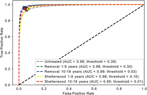
XGBoost modeling produced class probability maps for each of the 5 classes, provided as 5 separate 10-m resolution raster layers (summing to 100% for each pixel). Test data represented a 30% random sample of all pixels with known harvest types, including untreated forest, and was never used for model training or tuning. To the test data table we added the five predicted probability values, one for each class. We then used test data to calculate AUC-ROC (area under the receiver operator curve (ROC)) scores (Fielding and Bell 1997) to evaluate the ability of the model to discriminate between all pairs of classes (harvest types). We also used AUC-ROC plots to calculate the probability threshold that optimized the tradeoff between false positives and true positives. This threshold was estimated as the location on the ROC curve where the slope of the tangent line equaled 1 (e.g. maximum(sensitivity + specificity)) (Franklin 2010; Manel, Williams, and Ormerod 2001). Using these threshold values, we constructed a forest harvest classification map where the class mapped in each pixel was the class with the highest probability that exceeded the class threshold. Only 0.05% of all pixels lacked a class that exceeded one of the class probability thresholds, which were left unclassified.

We made an initial assessment of the classification results by visually inspecting mapped model predictions and quantifying accuracy for each class after applying the calculated thresholds. We inspected variable importance estimates and compared these with a priori understanding of how forest structure varied between predicted classes. Following good practice for classification assessment (Olofsson et al. 2014), we assembled test data into a confusion matrix and calculated overall accuracy, and errors of omission (false negatives) and commission (false positives) for each class, expressed as a percentage of all test data. A full report of accuracy results is presented in the Results section. We noted that areas classified as shelterwood often presented as spatially non-contiguous pixels or irregular patches within untreated forest. Although individually small, the frequency of these areas considerably increased false positive errors when accumulated across landscapes. Therefore, we opted to apply a majority filter at the scale of 10 × 10 pixels (100 m × 100 m). The majority filter removed isolated areas predicted as harvest but preserved the location of boundaries between larger harvest areas and untreated forest. We report error rates for results before and after applying the majority filter. In addition, we applied an interior buffer (at distances of 10, 20, 30, and 40 m) to the prediction map and removed these areas (representing forest edges) to reduce edge effects along the boundaries of the Dynamic World forest layer. These edge effects result from the subtle imprecision of the forest mask boundaries that unintentionally incorporate margin pixels of other classes (such as crops and yards) and which have the potential to add up cumulatively to considerable area. Due to the firm boundaries of public forest lands a similar analysis step was unnecessary.

3. Results

Initial investigations of relationships between LiDAR-derived forest metric summaries and forest harvest classes revealed strong associations, suggesting the potential for successful spatial modeling of timber harvests using LiDAR metrics as predictors (Figure 4). Both timber harvest types exhibited a large fraction of returns below 2 m in height, with overstory removal harvests showing this effect most strongly. Shelterwood harvests produced a bi-modal distribution in the fraction of returns below 2 m, with one peak centered on ~65% of returns below 2 m and a second centered on 100%. These results are consistent with the intent of a shelterwood harvest; the partial removal of canopy trees to create gaps that expose forest floor to sunlight, which in turn promote the establishment and growth of a regeneration layer. Consistent with these results, the p95 metric, which is an estimate of forest height (m), exhibited a bimodal distribution for both timber harvest types. Overstory removals exhibited a small peak at 20 m and a larger peak near the ground elevation. Meanwhile, shelterwood exhibited a large peak above 20 m and a small peak at ground elevation. For each harvest type, increasing harvest age was related to understory growth, with shorter trees growing faster than larger trees (i.e. the two distributions began to converge). In all cases, increasing age resulted in a reduction in the percent of returns from the near-ground level (<5 m), with near-ground returns becoming rare by 11 years post-harvest. Metrics such as the percent of returns <5 m (or voxel return densities within 5 m of the ground) were close to zero except in areas of recent overstory removals or other disturbance.

Quantitative accuracy assessment demonstrated many strengths of the model for mapping timber harvest types and age categories. First, AUC statistics were consistently close to 1 (Figure 5). Second, commission and omission error rates were generally low, with the highest commission errors found in the untreated and removal 1–9 year classes (6%) and the highest omission error in the shelterwood 10–18 year class (35%; Table 4). In general, the capability of the model to distinguish between the two age groups of removals and shelterwood harvests was marginally greater than the capability of the model to distinguish between each harvest type. When errors of omission and commission were committed, the 1–9 year classes were most likely to be misclassified as untreated or as the other 1–9 year age class. The removal 10–18 year class was most likely to be misclassified as untreated or removal 1–9 years. The shelterwood 10–18 year class was erroneously classified as one of the other classes in approximately 35% of cases, with the removal 10–18 year class the least frequent. Shelterwood was also more commonly confused with untreated forests than were removal harvests. Despite a high omission error rate, expressed in area units, omission errors in the shelterwood 10–18 year class were low because there were so few shelterwoods in this age class in the test data. However, commission errors of the shelterwood 1–9 year class into the untreated forest class were more extensive. With the exception of the shelterwood 10–18 year class omission errors (increased by 7%), the application of the majority filter greatly reduced both omission (by between 3.8% and 6.3%) and commission (by between 2.8% and 8.9%) errors among model classes (Table 4).

Table 4. Confusion matrix showing correct classification rates (diagonal elements) and error rates (off diagonal elements).

	Untreated	Removal 1–9 yrs	Removal 10–18 yrs	Shelterwood 1–9 yrs	Shelterwood 10–18 yrs	Row Total	Omission Error
Untreated	35.73%	0.51%	0.15%	0.37%	0.01%	36.8%	2.8% (8.1%)
Removal 1–9 yrs	0.27%	28.58%	0.05%	0.10%	0.002%	29.0%	1.5% (5.3%)
Removal 10–18 yrs	0.19%	0.41%	8.81%	0.02%	0.001%	9.4%	6.6% (12.4%)
Shelterwood 1–9 yrs	0.94%	0.45%	0.001%	18.70%	0.001%	20.1%	7.0% (13.3%)
Shelterwood 10–18 yrs	0.83%	0.47%	0.04%	0.30%	3.05%	4.7%	34.9% (27.9%)
Column Total	38.0%	30.4%	9.1%	19.5%	3.1%	100%
Commission Error	5.9% (9.0%)	6.0% (8.8%)	2.6% (9.8%)	4.1% (12.3%)	0.3% (9.2%)		OA = 94.9% (90.3%)

Columns are reference data and rows are modeled estimates. Error rates are calculated as the number of data points either correctly or incorrectly classified divided by the total number of test data. Errors of omission and commission are reported for each class after (and before) the application of the majority filter on the class prediction map. OA = overall accuracy after the majority filter (before the majority filter).

Figure 5. Receiver operating characteristic (ROC) plots and Area Under the Curve (AUC) for each class modeled. The threshold indicated for each class (circles) balances false and true positive error rates.

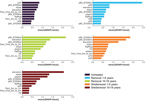
Mapped model predictions to the Poconos, PA Wilds, and Laurel Highlands regions produced primarily contiguous areas of untreated, mature forests. Model-predicted timber harvest boundaries were largely embedded within untreated forest matrices and exhibited patch sizes and spacing that would be expected for these landscapes (Figures 6, 7). The edges of predicted harvests showed clear delineation with untreated forest. A visual comparison with satellite imagery demonstrates that our model accurately predicted the presence of regenerated timber harvests that had regrown sufficiently to be virtually indistinguishable from untreated forest to the human eye (Figure 6). Comparison with polygons of timber harvest showed excellent visual accuracy, which was supported by model accuracy calculations (Table 4). Structural metrics important for these predictions varied among timber harvest type (Figure 8). The most important variable for predicting the presence of overstory removals (both age classes) was the standard deviation of the p99 canopy height at the 50 m focal distance (p99_STD50m). This metric is expected to be highest when canopy height varies greatly among adjacent 10 m pixels, which might be the case following an overstory removal harvest if scattered residual trees are retained (which is common practice). The density of LiDAR returns between 1 and 5 m from the ground surface was also an important variable for predicting overstory removal harvests 10–18 years old (specifically Perc_First_5m_to_2m and Perc_2m_to_1m metrics). Topographic variables (elevation, slope, and aspect) were important predictors, particularly for shelterwoods 10–18 years old. However, mapped predictions did not exhibit strong patterns related to topography, particularly after the application of the majority filter. The number of training data for each harvest type may have influenced this effect. For example, older shelterwood harvests are rare on the landscape. Given fewer training data, XGBoost might have a tendency to predict this rare class in areas with a similar topographic position as that of the limited training data.

Figure 6. Final classification map for two areas with exemplar forest harvests of both types and ages occurring on both sides of the private-public boundary. Comparison with airborne photography shows that many of the harvests mapped are not apparent in optical data. In other cases, harvested areas show up as areas with less shading (lighter) or more non-photosynthetic vegetation (browner) in aerial photos.

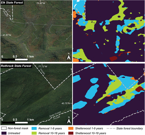
Figure 7. Predicted results for the PA wilds conservation area.

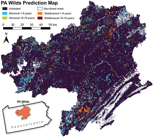
Figure 8. The top 10 most important metrics for each harvest class based on the mean SHAP values (Lundberg et al. 2020) from the XGBoost model. See Table 2 for definitions of each metric.

Model summaries of the untreated and harvested areas across the Poconos, PA Wilds, and Laurel Highlands indicated higher overstory removal rates in private lands (Table 5). However, we noted that a large portion of the harvested area occurred along forest edges. Assuming these were classification errors due to mixed pixel effects at the forest boundary, we applied an interior buffer (30 m in width) to the forest mask and focused remaining analysis on just the remaining “interior” forest area. For these interior forests, model summaries indicated near equal rates of harvest (across types and ages) between private and public lands. One exception to this general pattern, however, was in the Poconos region; wherein our model predicted that there was 42% less overstory removal 1–9 years old on private land (1.81%) than public land (3.13%) (Table 5). The other discrepancy occurred in the Laurel Highlands, where shelterwood 1–9-year-old harvests were twice as common in private than in public forests.

Table 5. Statistics for public and private forest lands for each class in the three key conservation areas across Pennsylvania.

Treatment class	Conservation area	% of public forest lands (total area)	% of private forest lands (total area)	% of private forest lands with 30m buffer (total area)	% change 0-30m buffer on private forest lands
Untreated	Laurel Highlands	92.59 (734 km^2)	84.87 (3466 km^2)	91.51 (956 km^2)	7.8
	PA Wilds	90.22 (5797 km^2)	87.47 (4008 km^2)	90.23 (2172 km^2)	3.2
	Poconos	95.93 (1182 km^2)	94.16 (3309 km^2)	97.55 (1195 km^2)	3.6
Removal 1–9 yrs	Laurel Highlands	4.48 (36 km^2)	12.39 (506 km^2)	4.16 (44 km^2)	−66.4
	PA Wilds	4.76 (306 km^2)	9.00 (413 km^2)	5.01 (121 km^2)	−44.4
	Poconos	3.13 (39 km^2)	5.34 (188 km^2)	1.81 (22 km^2)	−66.2
Removal 10–18 yrs	Laurel Highlands	1.06 (8.4 km^2)	0.63 (26 km^2)	0.80 (8.3 km^2)	26.3
	PA Wilds	1.01 (65 km^2)	1.01 (46 km^2)	1.33 (32 km^2)	31.0
	Poconos	0.24 (3.0 km^2)	0.14 (4.9 km^2)	0.17 (2.1 km^2)	21.5
Shelterwood 1–9 yrs	Laurel Highlands	1.59 (13 km^2)	2.07 (85 km^2)	3.43 (36 km^2)	65.1
	PA Wilds	3.79 (243 km^2)	2.48 (114 km^2)	3.38 (81 km^2)	36.2
	Poconos	0.62 (7.6 km^2)	0.35 (12 km^2)	0.47 (5.7 km^2)	32.6
Shelterwood 10–18 yrs	Laurel Highlands	0.28 (2.3 km^2)	0.045 (1.8 km^2)	0.110 (1.2 km^2)	147.3
	PA Wilds	0.22 (14 km^2)	0.035 (1.6 km^2)	0.060 (1.4 km^2)	70.2
	Poconos	0.09 (1.1 km^2)	0.005 (0.2 km^2)	0.008 (0.1 km^2)	78.3

Private lands were additionally assessed following the application of a 30-m interior buffer to remove any bias due to edge effects. Values in bold indicate a reduction in treatment class after applying the 30-m interior buffer to private forests.

4. Discussion

4.1. Assessment of the model for Pennsylvania forests

As the availability of LiDAR continues to increase rapidly across the globe, so too does the potential to leverage these data across broad spatial scales in support of conservation efforts and forest management initiatives (Dubayah and Drake 2000; Falkowski et al. 2009; Hansen et al. 2014). Results from the XGBoost model presented here provide a promising example of how coupling 3-dimensional LiDAR datasets with machine learning can produce accurate prediction maps across large areas that improve on established techniques as well as provide information about forest inventories that are often poorly monitored (Phillips and Blinn 2007). For example, accurately tracking and inventorying forest activity across private lands is notoriously difficult (Cohen, Spies, and Fiorella 1995; Tortini et al. 2019; Wicker 2002), yet forests on private lands provide vast economic and environmental benefits that cannot be quantified or optimized in the absence of high-quality data (Ciuzio et al. 2013; Litvaitis et al. 2021; Phillips and Blinn 2007).

In this study, we benefited from an extensive training dataset that documented the broad extent and timing of timber harvests collected across Pennsylvania state forests over the preceding 25 years. These data (including extensive areas of untreated forest) represented approximately 13% of all forested land in Pennsylvania. The spatial and structural diversity along with the magnitude of training data allowed the model to develop a comprehensive understanding of the range of LiDAR metrics both within and across the five targeted classes from throughout the state’s forest. In addition, improved model accuracy was likely achieved by targeting a limited number of timber harvest types to predict. This reduction in predictive classes was deliberate and derived from the fact that forest growth follows a continuum that differs based on a host of influencing factors (soil, light, moisture, species, etc.) that are not easily predicted (Belair and Ducey 2018; Gunn, Ducey, and Belair 2019). To attempt to predict, for example, a class for each year after a removal (e.g. 18 removal classes) would likely result in widespread misclassification among similar classes. The goal of our model was to minimize these boundaries while retaining useful information such as type of timber harvest and a simplified age structure (essentially young or old). Lastly, the model benefited from the structurally unique profiles of each forest class (Belair and Ducey 2018; Gunn, Ducey, and Belair 2019), in that the structural differences between a mature untreated forest, and removal and shelterwood harvests could be quantified with relative ease (Wilson and Sader 2002). This was especially true for the young shelterwood and removal classes, whereas the older shelterwood 10–18 year class was more likely to begin to resemble untreated forest as would be expected with increasing maturity.

Despite the overall accuracy of the predictive model, there remain confounding factors that have implications for the application and interpretation of the results. The simplification of the predictive classes in the model, largely driven by the limited number of timber harvest classes available in the training data, strictly limits the prediction of any given pixel to those classes. For example, the XGBoost model was not constructed to identify all types of timber harvest such as unsustainable practices like high-grading, whereby the most valuable and robust trees are removed from the forest (Fajvan, Grushecky, and Hassler 1998; Nyland 1992). This problematic harvesting technique is known to be pervasive throughout private lands in the eastern US and can, in some cases, produce a canopy structure similar to that of a shelterwood (Curtze et al. 2022b). In addition, the model makes no distinction between timber harvest canopy structures and those caused by natural events, such as spongy moth (Lymantria dispar), Hemlock Wooly Adelgid (Adelges tsugae) and Emerald Ash Borer (Agrilus planipennis), which have impacted large swaths of deciduous forest across Pennsylvania (Davidson, Gottschalk, and Johnson 1999; Klooster et al. 2014). Similarly, gaps within untreated forest can be created by tornado tracks, ice and snow damage, or, at the scale of a 10 × 10 m pixel, even tree throw could cause a pixel class prediction to change without any timber harvest intervention. The latter case was the major impetus for applying a 100 × 100 m majority filter across the prediction map, with the goal of removing high-frequency, isolated pixels, enabling a focus on patch sizes consistent with established thresholds for timber harvest. Given this, and regardless of the biologic or anthropogenic process involved, the model is in fact predicting areas with a forest structure similar to that of a recently harvested forest. It may be that non-timber related processes that produce early successional forest are equally beneficial from a conservation perspective across both public and private lands, so long as minimal area requirements are met by such natural disturbances (Shake et al. 2012). Notably, techniques that rely on temporal optical remote sensing (e.g. loss of leaf area) to map harvests might also identify natural disturbances as harvests and have historically been limited to delineating specific harvest types across restricted spatial extents (Stahl et al. 2023).

As conservation planners increasingly rely on implementing holistic stewardship and resource development plans across public and private lands, the need for comprehensive information on private forests is critical (Ciuzio et al. 2013; Lutter et al. 2019). The XGBoost model was used to predict timber harvests across both private and public forests to estimate current inventories of timber harvests and overall forest structures. Initial assessment of the abundance of timber harvests classes across public and private forests in three focal conservation regions revealed a larger than expected discrepancy between the removal 1–9 year class on private lands and that on public lands (Table 5). Due to the increased fragmentation of private forests by agriculture, transportation, and development, forest inventories are often complicated by considerable edge anomalies and small parcel size (Brooks 2003; Sampson and DeCoster 2000). These two factors combine to produce considerably higher perimeter-to-area ratios than those observed on public lands and can bias estimates where forest masks are even slightly inaccurate (Riitters, Coulston, and Wickham 2012). Results from interior buffering of our forest mask demonstrates this problem with the removal 1–9 year class dominating predictions along private forest margins and, ultimately, skewing any comparisons between public and private lands. Using the 30-m interior buffer on private lands produces results roughly consistent with previous estimates for the state based on Forest Inventory and Analysis data (PA-DCNR 2020).

However, two notable trends emerge from the comparison of private and public forests within the three focal conservation regions. First, our model indicates a relatively high incidence of shelterwood 1–9 years in private forests in the PA Wilds and Laurel Highlands regions (~3.5% of private forest lands). Shelterwood harvests tend to be less common on private lands, owing to their expense (Lanham et al. 2002). With that in mind, it seems likely that many apparent shelterwoods on private lands are actually high-graded stands (Curtze et al. 2022a, 2022b) or stands impacted by natural events (i.e. spongy moth mortality). High-grades, in some respects, are similar to shelterwood harvests in that they are a partial harvest of a forest stand (Belair and Ducey 2018; Curtze et al. 2022a, 2022b; Gunn, Ducey, and Belair 2019), however, the types/quality of trees removed and goal of these two harvest types are drastically different (Dey 2014; Nyland 1992). Second, there is a notable discrepancy between the area of predicted younger harvests and those of older harvests within each timber harvest class. For example, our model predicts a > 60% reduction in area of overstory removals 10–18 years old than overstory removals 1–9 years old across both ownership types. Whereas this discrepancy might be expected for shelterwood harvests, as shelterwoods rarely make it past ~10 years before being subject to an overstory removal, the dearth of older overstory removals compared to younger overstory removals is counter to expectations (Loftis 1990). Potential causes for this finding could include an actual increase in overstory removals over the past decade and/or an increase in tree mortality events due to forest disease. For example, a spongy moth outbreak in PA caused widespread defoliation in 2009–2010 (Tobin et al. 2012). As most of our LiDAR surveys were collected from 2020 or before, this timing would align with the potential increase of predicted young overstory removals as these trees began to decay and fall. Regardless of these discrepancies, these findings demonstrate the unprecedented value of having a spatially extensive and accurate predictive map for conservation management and future hypothesis testing (Pierzchała, Giguère, and Astrup 2018; White et al. 2016).

4.2. Utility for conservation and resource planners

The predictive timber harvest map generated by our model provides utility beyond just an accounting of class frequency and aerial coverage. The resulting map is both a tool and reference that can be used by conservation and/or natural resource planners to directly target sites for protection, harvest, and long-term observation at various spatial scales from local to regional (e.g. similar to the focal conservation regions targeted in this study) (Kangas et al. 2018; White et al. 2016). For ongoing studies in PA forests the predictive timber harvest map provides a baseline condition for private and public lands that can act as a foundation to investigate a host of environmental, ecological, and resource-related hypotheses that span spatial and temporal continuum (Banskota et al. 2014; Wulder et al. 2020). Lastly, for foresters and academics interested in predicting timber harvest patterns from large-scale LiDAR campaigns outside of PA, this study provides a proof of concept and technical guide to addressing similar questions across diverse forest environments and species-habitat couplings (White et al. 2013).

5. Conclusions and future work

Here, we demonstrate the application of a highly capable machine learning algorithm (XGBoost) and airborne LiDAR-derived metrics to successfully map timber harvest types and ages within most of the forested land area of Pennsylvania, USA and summarize these conditions across three focal conservation regions. Our primary conclusion is that the coupling of machine learning algorithms with campaign-style airborne LiDAR has strong potential to provide critical insight to natural resource managers interested in understanding the distribution and abundance of timber harvests across large spatial extents with multiple ownership domains. An accurate understanding of the amount and type and age of timber harvests conducted in a region can be used to guide conservation management, policy, and natural resource decisions (White et al. 2016; Wulder et al. 2020). Therefore, the value of the methods used here stem from the ability to discern structural differences among forests, which indicates the habitat suitability of forests for diverse animal species more directly than would a workflow based on temporal mapping of disturbance.

Future efforts should seek to further refine the analyses presented in this study by developing workflows that incorporate more specific training data. Such data might include information about the dominant tree species across the state (e.g. oak/hickory vs maple/beech/birch) and inclusion of a high-grade timber harvest class to potentially tease out predictive overlap with shelterwoods (Belair and Ducey 2018; Curtze et al. 2022b). In addition, continuous refinement of the model through field verification of the model predictions could provide regular accuracy improvement, especially if increasing class complexity were instituted (i.e. 1st vs. 2nd entry shelterwoods). Lastly, timber harvest maps like those developed here can be incorporated into wildlife species distribution and habitat models (Fiss et al. 2021; Martinuzzi et al. 2009; McAuley et al. 1996). Using LiDAR metrics and forest harvest data as model predictors will likely enable detailed maps of habitat that inherently depend on habitat relationships with forest harvests (Ciuzio et al. 2013; Litvaitis et al. 2021; McNeil et al. 2020). Such models would enable estimation of conservation outcomes resulting from different harvest scenarios, for example in the context of evaluating conservation plans. As the quantity and quality of LiDAR data increase (Beland et al. 2019), spatial modelers and conservation practitioners should leverage these advances in concert with machine learning techniques with the ultimate goal to improve adaptive management of healthy, biodiverse ecosystems (Simonson et al. 2014; Wulder et al. 2008).

Acknowledgments

This project was funded by a United States Department of Agriculture—Natural Resources Conservation Service grant (# 69-3A75-17-438) and a National Aeronautics and Space Administration grant (# NNX17AG41G). We are very grateful for the assistance of S. Guinn on early LiDAR processing efforts.

Disclosure statement

No potential conflict of interest was reported by the author(s).

Data availability statement

Due to the considerable size of (1) the data that support the findings of this study and (2) the resulting products, these data are only available from the corresponding author, G. Burch Fisher, upon reasonable request. All code associated with this project and specific package parameters needed for reproducibility can be found in the public GitHub repository for the project (https://github.com/burchfisher/ForestBirds).

Additional information

Funding

The work was supported by the National Aeronautics and Space Administration [NNX17AG41G]; USDA - Natural Resources Conservation Service [69-3A75-17-438].

References

- Achim, A., G. Moreau, N. C. Coops, J. N. Axelson, J. Barrette, S. Bédard, K. E. Byrne, et al. 2021. “The Changing Culture of Silviculture.” Forestry 95 (2): 143–23. https://doi.org/10.1093/forestry/cpab047.
- Arundel, S. T., A. N. Bulen, K. F. Adkins, R. E. Brown, A. J. Lowe, K. S. Mantey, and L. A. Phillips. 2018. “Assimilation of the National Elevation Dataset and Launch of the 3D Elevation Program Through the USGS Spatial Data Infrastructure.” International Journal of Cartography 4 (2): 129–150. https://doi.org/10.1080/23729333.2017.1288533.
- Atkins, J. W., G. Bohrer, R. T. Fahey, B. S. Hardiman, T. H. Morin, A. E. L. Stovall, N. Zimmerman, and C. M. Gough. 2018. “Quantifying Vegetation and Canopy Structural Complexity from Terrestrial Li DAR Data Using the Forestr R Package.” Methods in Ecology and Evolution 9 (10): 2057–2066. https://doi.org/10.1111/2041-210X.13061.
- Banskota, A., N. Kayastha, M. J. Falkowski, M. A. Wulder, R. E. Froese, and J. C. White. 2014. “Forest Monitoring Using Landsat Time Series Data: A Review.” Canadian Journal of Remote Sensing 40 (5): 362–384. https://doi.org/10.1080/07038992.2014.987376.
- Barrett, J. W. 1962. “Regional Silviculture of the United States.” Soil Science 94 (2): 134. https://doi.org/10.1097/00010694-196208000-00016.
- Baskent, E. Z., and S. Keles. 2005. “Spatial Forest Planning: A Review.” Ecological Modelling 188 (2–4): 145–173. https://doi.org/10.1016/j.ecolmodel.2005.01.059.
- Belair, E. P., and M. J. Ducey. 2018. “Patterns in Forest Harvesting in New England and New York: Using FIA Data to Evaluate Silvicultural Outcomes.” Journal of Forestry 116 (3): 273–282. https://doi.org/10.1093/jofore/fvx019.
- Beland, M., G. Parker, B. Sparrow, D. Harding, L. Chasmer, S. Phinn, A. Antonarakis, and A. Strahler. 2019. “On Promoting the Use of Lidar Systems in Forest Ecosystem Research.” Forest Ecology & Management 450:117484. https://doi.org/10.1016/j.foreco.2019.117484.
- Bergen, K. M., S. J. Goetz, R. O. Dubayah, G. M. Henebry, C. T. Hunsaker, M. L. Imhoff, R. F. Nelson, G. G. Parker, and V. C. Radeloff. 2009. “Remote Sensing of Vegetation 3-D Structure for Biodiversity and Habitat: Review and Implications for Lidar and Radar Spaceborne Missions.” Journal of Geophysical Research: Biogeosciences 114 (G2): 114. https://doi.org/10.1029/2008jg000883.
- Boutin, S., and D. Hebert. 2002. “Landscape Ecology and Forest Management: Developing an Effective Partnership.” Ecological Applications 12 (2): 390–397. https://doi.org/10.1890/1051-0761(2002)012[0390:LEAFMD]2.0.CO;2.
- Boves, T. J., D. A. Buehler, J. Sheehan, P. B. Wood, A. D. Rodewald, J. L. Larkin, P. D. Keyser, et al. 2013. “Emulating Natural Disturbances for Declining Late-Successional Species: A Case Study of the Consequences for Cerulean Warblers (Setophaga Cerulea).” PLOS ONE 8 (1): e52107. https://doi.org/10.1371/journal.pone.0052107.
- Brooks, R. T. 2003. “Abundance, Distribution, Trends, and Ownership Patterns of Early-Successional Forests in the Northeastern United States.” Forest Ecology & Management 185 (1–2): 65–74. https://doi.org/10.1016/S0378-1127(03)00246-9.
- Brown, C. F., S. P. Brumby, B. Guzder-Williams, T. Birch, S. B. Hyde, J. Mazzariello, W. Czerwinski, et al. 2022. “Dynamic World, Near Real-Time Global 10 M Land Use Land Cover Mapping.” Scientific Data 9 (1): 1–17. https://doi.org/10.1038/s41597-022-01307-4.
- Brubaker, K. M., S. E. Johnson, J. Brinks, and L. P. Leites. 2014. “Estimating Canopy Height of Deciduous Forests at a Regional Scale with Leaf-Off, Low Point Density LiDAR.” Can J Remote Sens 40 (2): 123–134. https://doi.org/10.1080/07038992.2014.943392.
- Chen, T., and C. Guestrin. 2016. “XGBoost: A Scalable Tree Boosting System.” Proceedings of the 22nd ACM SIGKDD International Conference on Knowledge Discovery and Data Mining, KDD ’16, 785–794. New York, NY: Association for Computing Machinery.
- Ciuti, S., H. Tripke, P. Antkowiak, R. S. Gonzalez, C. F. Dormann, M. Heurich, and D. Warton. 2018. “An Efficient Method to Exploit Li DAR Data in Animal Ecology.” Methods in Ecology and Evolution 9 (4): 893–904. https://doi.org/10.1111/2041-210X.12921.
- Ciuzio, E., W. L. Hohman, B. Martin, M. D. Smith, S. Stephens, A. M. Strong, and T. Vercauteren. 2013. “Opportunities and Challenges to Implementing Bird Conservation on Private Lands.” Wildlife Society Bulletin 37 (2): 267–277. https://doi.org/10.1002/wsb.266.
- Cohen, W. B., T. A. Spies, and M. Fiorella. 1995. “Estimating the Age and Structure of Forests in a Multi-Ownership Landscape of Western Oregon, USA.” International Journal of Remote Sensing 16 (4): 721–746. https://doi.org/10.1080/01431169508954436.
- Coops, N. C., P. Tompalski, T. R. H. Goodbody, M. Queinnec, J. E. Luther, D. K. Bolton, J. C. White, M. A. Wulder, O. R. van Lier, and T. Hermosilla. 2021. “Modelling Lidar-Derived Estimates of Forest Attributes Over Space and Time: A Review of Approaches and Future Trends.” Remote Sensing of Environment 260:112477. https://doi.org/10.1016/j.rse.2021.112477.
- Coops, N. C., P. Tompaski, W. Nijland, G. J. M. Rickbeil, S. E. Nielsen, C. W. Bater, and J. J. Stadt. 2016. “A Forest Structure Habitat Index Based on Airborne Laser Scanning Data.” Ecological Indicators 67:346–357. https://doi.org/10.1016/j.ecolind.2016.02.057.
- Corte, A. P. D., D. V. Souza, F. E. Rex, C. R. Sanquetta, M. Mohan, C. A. Silva, A. M. A. Zambrano, et al. 2020. “Forest Inventory with High-Density UAV-Lidar: Machine Learning Approaches for Predicting Individual Tree Attributes.” Computers and Electronics in Agriculture 179:105815. https://doi.org/10.1016/j.compag.2020.105815.
- Curtze, A. C., A. B. Muth, J. L. Larkin, and L. P. Leites. 2022a. “Decision Support Tools to Inform the Rehabilitation and Management of High Graded Forests.” Journal of Forestry 120 (5): 527–542. https://doi.org/10.1093/jofore/fvab077.
- Curtze, A. C., A. B. Muth, J. L. Larkin, and L. P. Leites. 2022b. “Seeing Past the Green: Structure, Composition, and Biomass Differences in High Graded and Silviculture-Managed Forests of Similar Stand Density.” Forest Ecology & Management 526:120598. https://doi.org/10.1016/j.foreco.2022.120598.
- Davidson, C. B., K. W. Gottschalk, and J. E. Johnson. 1999. “Tree Mortality Following Defoliation by the European Gypsy Moth (Lymantria Dispar L.) in the United States: A Review.” Forest Science 45 (1): 74–84. https://doi.org/10.1093/forestscience/45.1.74.
- Dey, D. C. 2014. “Sustaining Oak Forests in Eastern North America: Regeneration and Recruitment, the Pillars of Sustainability.” Forest Science 60 (5): 926–942. https://doi.org/10.5849/forsci.13-114.
- Dickinson, Y., E. K. Zenner, and D. Miller. 2014. “Examining the Effect of Diverse Management Strategies on Landscape Scale Patterns of Forest Structure in Pennsylvania Using Novel Remote Sensing Techniques.” Canadian Journal of Forest Research 44 (4): 301–312. https://doi.org/10.1139/cjfr-2013-0315.
- Dubayah, R. O., and J. B. Drake. 2000. “Lidar Remote Sensing for Forestry.” Journal of Forestry 98 (6): 44–46. https://doi.org/10.1093/jof/98.6.44.
- Fajvan, M. A., S. T. Grushecky, and C. C. Hassler. 1998. “The Effects of Harvesting Practices on West Virginia’s Wood Supply.” Journal of Forestry 96 (5): 33–39. https://doi.org/10.1093/jof/96.5.33.
- Falkowski, M. J., J. S. Evans, S. Martinuzzi, P. E. Gessler, and A. T. Hudak. 2009. “Characterizing Forest Succession with Lidar Data: An Evaluation for the Inland Northwest, USA.” Remote Sensing of Environment 113 (5): 946–956. https://doi.org/10.1016/j.rse.2009.01.003.
- Farrell, S. L., B. A. Collier, K. L. Skow, A. M. Long, A. J. Campomizzi, M. L. Morrison, and K. B. Hays. 2013. “Using LiDAR‐Derived Vegetation Metrics for High‐Resolution, Species Distribution Models for Conservation Planning.” Ecosphere 4 (3): 1–18. https://doi.org/10.1890/ES12-000352.1.
- Fedrigo, M., G. J. Newnham, N. C. Coops, D. S. Culvenor, D. K. Bolton, and C. R. Nitschke. 2018. “Predicting Temperate Forest Stand Types Using Only Structural Profiles from Discrete Return Airborne Lidar.” ISPRS Journal of Photogrammetry and Remote Sensing 136:106–119. https://doi.org/10.1016/j.isprsjprs.2017.11.018.
- Fielding, A. H., and J. F. Bell. 1997. “A Review of Methods for the Assessment of Prediction Errors in Conservation Presence/Absence Models.” Environmental Conservation 24 (1): 38–49. https://doi.org/10.1017/S0376892997000088.
- Fiss, C. J., D. J. McNeil, A. D. Rodewald, J. E. Duchamp, and J. L. Larkin. 2020. “Post-Fledging Golden-Winged Warblers Require Forests with Multiple Stand Developmental Stages.” Condor 122. https://doi.org/10.1093/condor/duaa052.
- Fiss, C., D. McNeil, A. Rodewald, D. Heggenstaller, and J. L. Larkin. 2021. “Cross-Scale Habitat Selection Reveals Within-Stand Structural Requirements for Fledgling Golden-Winged Warblers.” Avian Conservation & Ecology 16 (1). https://doi.org/10.5751/ACE-01807-160116.
- Frank, B., F. Mauro, H. Temesgen, and K. R. Ford. 2019. “Analysis of Classification Methods for Identifying Stands for Commercial Thinning Using LiDAR.” Canadian Journal of Remote Sensing 45 (5): 673–690. https://doi.org/10.1080/07038992.2019.1670051.
- Franklin, J. 2010. Mapping Species Distributions: Spatial Inference and Prediction. Cambridge: Cambridge University Press.
- Gao, Y., M. Skutsch, J. Paneque-Gálvez, and A. Ghilardi. 2020. “Remote Sensing of Forest Degradation: A Review.” Environmental Research Letters 15 (10): 103001. https://doi.org/10.1088/1748-9326/abaad7.
- Goetz, S. J., D. Steinberg, M. G. Betts, R. T. Holmes, P. J. Doran, R. Dubayah, and M. Hofton. 2010. “Lidar Remote Sensing Variables Predict Breeding Habitat of a Neotropical Migrant Bird.” Ecology 91 (6): 1569–1576. https://doi.org/10.1890/09-1670.1.
- Greenberg, C. H., B. Collins, F. R. Thompson, and W. H. McNab. 2011. “Introduction: What are Early Successional Habitats, Why are They Important, and How Can They Be Sustained?” In Sustaining Young Forest Communities: Ecology and Management of Early Successional Habitats in the Central Hardwood Region, USA, edited by C. Greenberg, B. Collins, and F. Thompson III, 1–10. Dordrecht, Netherlands: Springer.
- Gunn, J. S., M. J. Ducey, and E. Belair. 2019. “Evaluating Degradation in a North American Temperate Forest.” Forest Ecology & Management 432:415–426. https://doi.org/10.1016/j.foreco.2018.09.046.
- Hansen, A. J., L. B. Phillips, R. Dubayah, S. Goetz, and M. Hofton. 2014. “Regional-Scale Application of Lidar: Variation in Forest Canopy Structure Across the Southeastern US.” Forest Ecology & Management 329:214–226. https://doi.org/10.1016/j.foreco.2014.06.009.
- Hansen, M. C., P. V. Potapov, R. Moore, M. Hancher, S. A. Turubanova, A. Tyukavina, D. Thau, et al. 2013. “High-Resolution Global Maps of 21st-Century Forest Cover Change.” Science 342 (6160): 850–853. https://doi.org/10.1126/science.1244693.
- Hardiman, B. S., E. A. LaRue, J. W. Atkins, R. T. Fahey, F. W. Wagner, and C. M. Gough. 2018. “Spatial Variation in Canopy Structure Across Forest Landscapes.” Forest Trees Livelihoods 9 (8): 474. https://doi.org/10.3390/f9080474.
- Hermosilla, T., M. A. Wulder, J. C. White, N. C. Coops, and G. W. Hobart. 2018. “Disturbance-Informed Annual Land Cover Classification Maps of Canada’s Forested Ecosystems for a 29-Year Landsat Time Series.” Canadian Journal of Remote Sensing 44 (1): 67–87. https://doi.org/10.1080/07038992.2018.1437719.
- Jarron, L. R., T. Hermosilla, N. C. Coops, M. A. Wulder, J. C. White, G. W. Hobart, and D. G. Leckie. 2016. “Differentiation of Alternate Harvesting Practices Using Annual Time Series of Landsat Data.” Forest Trees Livelihoods 8 (1): 15. https://doi.org/10.3390/f8010015.
- Kangas, A., T. Gobakken, S. Puliti, M. Hauglin, and E. Naesset. 2018. “Value of Airborne Laser Scanning and Digital Aerial Photogrammetry Data in Forest Decision Making.” Silva Fennica 52 (1). https://doi.org/10.14214/sf.9923.
- King, D. I., R. M. Degraaf, M.-L. Smith, and J. P. Buonaccorsi. 2006. “Habitat Selection and Habitat-Specific Survival of Fledgling Ovenbirds (Seiurus Aurocapilla).” Journal of Zoology 269 (4): 414–421. https://doi.org/10.1111/j.1469-7998.2006.00158.x.
- King, D. I., and S. Schlossberg. 2014. “Synthesis of the Conservation Value of the Early-Successional Stage in Forests of Eastern North America.” Forest Ecology & Management 324:186–195. https://doi.org/10.1016/j.foreco.2013.12.001.
- Klooster, W. S., D. A. Herms, K. S. Knight, C. P. Herms, D. G. McCullough, A. Smith, K. J. K. Gandhi, and J. Cardina. 2014. “Ash (Fraxinus Spp.) Mortality, Regeneration, and Seed Bank Dynamics in Mixed Hardwood Forests Following Invasion by Emerald Ash Borer (Agrilus Planipennis).” Biological Invasions 16 (4): 859–873. https://doi.org/10.1007/s10530-013-0543-7.
- Lanham, J. D., P. D. Keyser, P. H. Brose, and D. H. Van Lear. 2002. “Oak Regeneration Using the Shelterwood-Burn Technique: Management Options and Implications for Songbird Conservation in the Southeastern United States.” Forest Ecology & Management 155 (1–3): 143–152. https://doi.org/10.1016/S0378-1127(01)00554-0.
- LaRue, E. A., R. Fahey, T. L. Fuson, J. R. Foster, J. H. Matthes, K. Krause, and B. S. Hardiman. 2022. “Evaluating the Sensitivity of Forest Structural Diversity Characterization to LiDAR Point Density.” Ecosphere 13 (9): e4209. https://doi.org/10.1002/ecs2.4209.
- Litvaitis, J. A., J. L. Larkin, D. J. McNeil, D. Keirstead, and B. Costanzo. 2021. “Addressing the Early-Successional Habitat Needs of At-Risk Species on Privately Owned Lands in the Eastern United States.” The Land 10 (11): 1116. https://doi.org/10.3390/land10111116.
- Loftis, D. L. 1990. “A Shelterwood Method for Regenerating Red Oak in the Southern Appalachians.” Forest Science 36 (4): 917–929. https://doi.org/10.1093/forestscience/36.4.917.
- Lundberg, S. M., G. Erion, H. Chen, A. DeGrave, J. M. Prutkin, B. Nair, R. Katz, J. Himmelfarb, N. Bansal, and S.-I. Lee. 2020. “From Local Explanations to Global Understanding with Explainable AI for Trees.” Nature Machine Intelligence 2 (1): 56–67. https://doi.org/10.1038/s42256-019-0138-9.
- Lutter, S. H., A. A. Dayer, A. D. Rodewald, D. J. McNeil, and J. L. Larkin. 2019. “Early Successional Forest Management on Private Lands As a Coupled Human and Natural System.” Forest Trees Livelihoods 10 (6): 499. https://doi.org/10.3390/f10060499.
- Maltamo, M., H. Kinnunen, A. Kangas, and L. Korhonen. 2020. “Predicting Stand Age in Managed Forests Using National Forest Inventory Field Data and Airborne Laser Scanning.” Forest Ecosystems 7 (1): 44. https://doi.org/10.1186/s40663-020-00254-z.
- Manel, S., H. C. Williams, and S. J. Ormerod. 2001. “Evaluating Presence–Absence Models in Ecology: The Need to Account for Prevalence.” The Journal of Applied Ecology 38 (5): 921–931. https://doi.org/10.1046/j.1365-2664.2001.00647.x.
- Martinuzzi, S., L. A. Vierling, W. A. Gould, M. J. Falkowski, J. S. Evans, A. T. Hudak, and K. T. Vierling. 2009. “Mapping Snags and Understory Shrubs for a LiDAR-Based Assessment of Wildlife Habitat Suitability.” Remote Sensing of Environment 113 (12): 2533–2546. https://doi.org/10.1016/j.rse.2009.07.002.
- Matasci, G., T. Hermosilla, M. A. Wulder, J. C. White, N. C. Coops, G. W. Hobart, and H. S. J. Zald. 2018. “Large-Area Mapping of Canadian Boreal Forest Cover, Height, Biomass and Other Structural Attributes Using Landsat Composites and Lidar Plots.” Remote Sensing of Environment 209:90–106. https://doi.org/10.1016/j.rse.2017.12.020.
- McAuley, D. G., J. R. Longcore, G. F. Sepik, and G. W. Pendleton. 1996. “Habitat Characteristics of American Woodcock Nest Sites on a Managed Area in Maine.” The Journal of Wildlife Management 60 (1): 138–148. https://doi.org/10.2307/3802048.
- McNeil, D. J., K. R. Aldinger, M. H. Bakermans, J. A. Lehman, A. C. Tisdale, J. A. Jones, P. B. Wood, et al. 2017. “An Evaluation and Comparison of Conservation Guidelines for an At-Risk Migratory Songbird.” Global Ecology and Conservation 9:90–103. https://doi.org/10.1016/j.gecco.2016.12.006.
- McNeil, D. J., G. Fisher, C. J. Fiss, A. J. Elmore, M. C. Fitzpatrick, J. W. Atkins, J. Cohen, and J. L. Larkin. 2023. “Using Aerial LiDAR to Assess Regional Availability of Potential Habitat for a Conservation Dependent Forest Bird.” Forest Ecology & Management 540:121002. https://doi.org/10.1016/j.foreco.2023.121002.
- McNeil, D. J., C. J. Fiss, E. M. Wood, J. E. Duchamp, M. Bakermans, and J. L. Larkin. 2018. “Using a Natural Reference System to Evaluate Songbird Habitat Restoration.” Avian Conservation & Ecology Oiseaux 13. https://doi.org/10.5751/ace-01193-130122.
- McNeil, D. J., A. D. Rodewald, V. Ruiz‐Gutierrez, K. E. Johnson, M. Strimas‐Mackey, S. Petzinger, O. J. Robinson, G. E. Soto, A. A. Dhondt, and J. L. Larkin. 2020. “Multiscale Drivers of Restoration Outcomes for an Imperiled Songbird.” Restoration Ecology 28 (4): 880–891. https://doi.org/10.1111/rec.13147.
- Moore, J., and Y. Lin. 2019. “Determining the Extent and Drivers of Attrition Losses from Wind Using Long-Term Datasets and Machine Learning Techniques.” Forestry: An International Journal of Forest Research 92 (4): 425–435. https://doi.org/10.1093/forestry/cpy047.
- North American Bird Conservation Initiative, U.S. Committee. 2013. The State of The Birds 2013 Report on Private Lands. Washington, DC: U.S. Department of Interior.
- Nyland, R. D. 1992. “Exploitation and Greed in Eastern Hardwood Forests.” Journal of Forestry 90 (1): 33–37. https://doi.org/10.1093/jof/90.1.33.
- Olofsson, P., G. M. Foody, M. Herold, S. V. Stehman, C. E. Woodcock, and M. A. Wulder. 2014. “Good Practices for Estimating Area and Assessing Accuracy of Land Change.” Remote Sensing of Environment 148:42–57. https://doi.org/10.1016/j.rse.2014.02.015.
- O’Neil-Dunne, J., S. MacFaden, and A. Royar. 2014. “A Versatile, Production-Oriented Approach to High-Resolution Tree-Canopy Mapping in Urban and Suburban Landscapes Using GEOBIA and Data Fusion.” Remote Sensing 6 (12): 12837–12865. https://doi.org/10.3390/rs61212837.
- PA-DCNR. 2020. Pennsylvania Forest Action Plan. Harrisburg, PA: Pennsylvania Department of Conservation and Natural Resources.
- Parent, C. J., and F. Hernández. 2021, “The Landscape Perspective in WIldlife and Habitat Management.” Wildlife Management and Landscapes: Principles and Applications, edited by W. F. Porter, C. J. Parent, R. A. Stewart, andf D. M. Williams, 3–18. Baltimore: Johns Hopins University Press. https://doi.org/10.1353/book.83118.
- Pasquarella, V. J., C. E. Holden, L. Kaufman, C. E. Woodcock, H. Nagendra, and K. He. 2016. “From Imagery to Ecology: Leveraging Time Series of All Available Landsat Observations to Map and Monitor Ecosystem State and Dynamics.” Remote Sensing in Ecology and Conservation 2 (3): 152–170. https://doi.org/10.1002/rse2.24.
- Phillips, M. J., and C. R. Blinn. 2007. “Practices Evaluated and Approaches Used to Select Sites for Monitoring the Application of Best Management Practices: A Regional Summary.” Journal of Forestry 105 (4): 179–183. https://doi.org/10.1093/jof/105.4.179.
- Pierzchała, M., P. Giguère, and R. Astrup. 2018. “Mapping Forests Using an Unmanned Ground Vehicle with 3D LiDAR and Graph-SLAM.” Computers and Electronics in Agriculture 145:217–225. https://doi.org/10.1016/j.compag.2017.12.034.
- Pressey, R. L., M. Cabeza, M. E. Watts, R. M. Cowling, and K. A. Wilson. 2007. “Conservation Planning in a Changing World.” Trends in Ecology & Evolution 22 (11): 583–592. https://doi.org/10.1016/j.tree.2007.10.001.
- Racine, E. B., N. C. Coops, B. St-Onge, and J. Bégin. 2013. “Estimating Forest Stand Age from LiDAR-Derived Predictors and Nearest Neighbor Imputation.” Forest Science 60 (1): 128–136. https://doi.org/10.5849/forsci.12-088.
- Raybuck, D. W., J. L. Larkin, S. H. Stoleson, and T. J. Boves. 2019. “Radio-Tracking Reveals Insight into Survival and Dynamic Habitat Selection of Fledgling Cerulean Warblers.” The Condor 122 (1): duz063. https://doi.org/10.1093/condor/duz063.
- Riitters, K. H., J. W. Coulston, and J. D. Wickham. 2012. “Fragmentation of Forest Communities in the Eastern United States.” Forest Ecology & Management 263:85–93. https://doi.org/10.1016/j.foreco.2011.09.022.
- Roussel, J.-R., D. Auty, N. C. Coops, P. Tompalski, T. R. H. Goodbody, A. S. Meador, J.-F. Bourdon, F. de Boissieu, and A. Achim. 2020. “LidR: An R Package for Analysis of Airborne Laser Scanning (ALS) Data.” Remote Sensing of Environment 251:112061. https://doi.org/10.1016/j.rse.2020.112061.
- Sabol, D. E., A. R. Gillespie, J. B. Adams, M. O. Smith, and C. J. Tucker. 2002. “Structural Stage in Pacific Northwest Forests Estimated Using Simple Mixing Models of Multispectral Images.” Remote Sensing of Environment 80 (1): 1–16. https://doi.org/10.1016/S0034-4257(01)00245-0.
- Sallabanks, R., and E. B. Arnett. 2005. Accommodating Birds in Managed Forests of North America: A Review of Bird–Forestry Relationships. Bird Conservation Implementation and Integration in the Americas. US Forest Service General Technical Report PSW-191. Albany, California, USA 345–372.
- Sampson, N., and L. DeCoster. 2000. “Forest Fragmentation: Implications for Sustainable Private Forests.” Journal of Forestry 98 (3): 4–8. https://doi.org/10.1093/jof/98.3.4.
- Sanchez-Lopez, N., L. Boschetti, and A. T. Hudak. 2019. “Reconstruction of the Disturbance History of a Temperate Coniferous Forest Through Stand-Level Analysis of Airborne LiDAR Data.” Forestry: An International Journal of Forest Research 93:38–55. https://doi.org/10.1093/forestry/cpz048.
- Sauer, J. R., W. A. Link, J. E. Fallon, K. L. Pardieck, and D. J. Ziolkowski. 2013. “The North American Breeding Bird Survey 1966–2011: Summary Analysis and Species Accounts.” North American Fauna 79:1–32. https://doi.org/10.3996/nafa.79.0001.
- Schwenk, W. S., and T. M. Donovan. 2011. “A Multispecies Framework for Landscape Conservation Planning.” Conservation Biology 25 (5): 1010–1021. https://doi.org/10.1111/j.1523-1739.2011.01723.x.
- Senf, C., D. Pflugmacher, P. Hostert, and R. Seidl. 2017. “Using Landsat Time Series for Characterizing Forest Disturbance Dynamics in the Coupled Human and Natural Systems of Central Europe.” ISPRS Journal of Photogrammetry & Remote Sensing 130:453–463. https://doi.org/10.1016/j.isprsjprs.2017.07.004.
- Shake, C. S., C. E. Moorman, J. D. Riddle, and M. R. Burchell. 2012. “Influence of Patch Size and Shape on Occupancy by Shrubland Birds.” The Condor 114 (2): 268–278. https://doi.org/10.1525/cond.2012.110107.
- Shifley, S. R., W. K. Moser, D. J. Nowak, P. D. Miles, B. J. Butler, F. X. Aguilar, R. D. DeSantis, and E. J. Greenfield. 2014. “Five Anthropogenic Factors That Will Radically Alter Forest Conditions and Management Needs in the Northern United States.” Forest Science 60 (5): 914–925. https://doi.org/10.5849/forsci.13-153.
- Simonson, W. D., H. D. Allen, D. A. Coomes, and A. Tatem. 2014. “Applications of Airborne Lidar for the Assessment of Animal Species Diversity.” Methods in Ecology and Evolution 5 (8): 719–729. https://doi.org/10.1111/2041-210X.12219.
- Stahl, A. T., R. Andrus, J. A. Hicke, A. T. Hudak, B. C. Bright, and A. J. H. Meddens. 2023. “Automated Attribution of Forest Disturbance Types from Remote Sensing Data: A Synthesis.” Remote Sensing of Environment 285:113416. https://doi.org/10.1016/j.rse.2022.113416.
- Thom, D., and W. S. Keeton. 2020. “Disturbance-Based Silviculture for Habitat Diversification: Effects on Forest Structure, Dynamics, and Carbon Storage.” Forest Ecology & Management 469:118132. https://doi.org/10.1016/j.foreco.2020.118132.
- Tobin, P. C., B. B. Bai, D. A. Eggen, and D. S. Leonard. 2012. “The Ecology, Geopolitics, and Economics of Managing Lymantria Dispar in the United States.” International Journal of Pest Management 58 (3): 195–210. https://doi.org/10.1080/09670874.2011.647836.
- Tortini, R., A. L. Mayer, T. Hermosilla, N. C. Coops, and M. A. Wulder. 2019. “Using Annual Landsat Imagery to Identify Harvesting Over a Range of Intensities for Non-Industrial Family Forests.” Landscape and Urban Planning 188:143–150. https://doi.org/10.1016/j.landurbplan.2018.04.012.
- Twedt, D. J. 2020. “Influence of Forest Harvest Severity and Time Since Perturbation on Conservation of North American Birds.” Forest Ecology & Management 458:117742. https://doi.org/10.1016/j.foreco.2019.117742.
- US Fish & Wildlife Service. 2006. Strategic Habitat Conservation: A Report from the National Ecological Assessment Team. Washington, DC: US Fish and Wildlife Service.
- White, J. C., N. C. Coops, M. A. Wulder, M. Vastaranta, T. Hilker, and P. Tompalski. 2016. “Remote Sensing Technologies for Enhancing Forest Inventories: A Review.” Canadian Journal of Remote Sensing 42 (5): 619–641. https://doi.org/10.1080/07038992.2016.1207484.
- White, J. C., M. A. Wulder, T. Hermosilla, N. C. Coops, and G. W. Hobart. 2017. “A Nationwide Annual Characterization of 25 Years of Forest Disturbance and Recovery for Canada Using Landsat Time Series.” Remote Sensing of Environment 194:303–321. https://doi.org/10.1016/j.rse.2017.03.035.
- White, J. C., M. A. Wulder, A. Varhola, M. Vastaranta, N. C. Coops, B. D. Cook, D. Pitt, and M. Woods. 2013. “A Best Practices Guide for Generating Forest Inventory Attributes from Airborne Laser Scanning Data Using an Area-Based Approach.” The Forestry Chronicle 89 (6): 722–723. https://doi.org/10.5558/tfc2013-132.
- Wicker, G. 2002. Motivation for Private Forest Landowners. Southern Forest Resource Assessment, Wear, DN and G. John. Gen. Tech. Rep. SRS-53. Ashville, NC: US Department.
- Wilson, E. H., and S. A. Sader. 2002. “Detection of Forest Harvest Type Using Multiple Dates of Landsat TM Imagery.” Remote Sensing of Environment 80 (3): 385–396. https://doi.org/10.1016/S0034-4257(01)00318-2.
- Wood, P., J. Sheehan, P. D. Keyser, D. A. Buehler, J. Larkin, A. D. Rodewald, S. H. Stoleson, et al. 2013. “Management Guidelines for Enhancing Cerulean Warbler Breeding Habitat in Appalachian Hardwood Forests.” 28. The Plains, Virginia: American Bird Conservancy.
- Wulder, M. A., C. W. Bater, N. C. Coops, T. Hilker, and J. C. White. 2008. “The Role of LiDAR in Sustainable Forest Management.” The Forestry Chronicle 84 (6): 807–826. https://doi.org/10.5558/tfc84807-6.
- Wulder, M. A., T. Hermosilla, J. C. White, and N. C. Coops. 2020. “Biomass Status and Dynamics Over Canada’s Forests: Disentangling Disturbed Area from Associated Aboveground Biomass Consequences.” Environmental Research Letters 15 (9): 094093. https://doi.org/10.1088/1748-9326/ab8b11.
- Wulder, M. A., R. S. Skakun, W. A. Kurz, and J. C. White. 2004. “Estimating Time Since Forest Harvest Using Segmented Landsat ETM+ Imagery.” Remote Sensing of Environment 93 (1–2): 179–187. https://doi.org/10.1016/j.rse.2004.07.009.
- Yu, J.-W., Y.-W. Yoon, W.-K. Baek, and H.-S. Jung. 2021. “Forest Vertical Structure Mapping Using Two-Seasonal Optic Images and LiDAR DSM Acquired from UAV Platform Through Random Forest, XGBoost, and Support Vector Machine Approaches.” Remote Sensing 13 (21): 4282. https://doi.org/10.3390/rs13214282.
- Zhu, Z., J. Zhang, Z. Yang, A. H. Aljaddani, W. B. Cohen, S. Qiu, and C. Zhou. 2020. “Continuous Monitoring of Land Disturbance Based on Landsat Time Series.” Remote Sensing of Environment 238:111116. https://doi.org/10.1016/j.rse.2019.03.009.