Dynamic flood mapping by a normalized probabilistic classification method using satellite radar amplitude time series

ABSTRACT

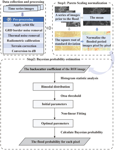
Owing to the vast development of Synthetic Aperture Radar (SAR), especially the improvement of spatio-temporal resolution, observing and quantifying the complex and dynamic flood process becomes increasingly feasible. Utilizing the Sentinel-1 Ground Range Detected (GRD) dataset, we proposed an improved probabilistic flood mapping method combining image Pareto Scaling (PS) normalization and Bayesian probability estimation. We validated our method during a flood event in Xinjiang County, Shaanxi Province of China in October 2021 using a high spatial resolution (0.1 m) Unmanned Aerial Vehicle (UAV) image. The overall reliability of the new method agrees 95% to the UAV measurements and achieves the highest accuracy (85.2%) when compared to the Sentinel-1 dual-polarized water index (SDWI) threshold method and the Z-score method. Our results distinguished four flood stages: flood emergence, peak, receding, and disappearance, which provide valuable insights into the dynamic change process of floods. Notably, we observed that pixels with different flood probabilities exhibited distinct temporal characteristics. The extremely high probability pixel experienced rapid fluctuations, while the medium probability pixel showed more gradual changes over time. We believe our proposed method can enhance our understanding of flood-prone areas and their dynamics so that decision-makers can develop targeted mitigation measures and response plans.

KEYWORDS:

• Flood mapping
• change detection
• satellite radar amplitude
• flood evolution

1. Introduction

Global warming has intensified the frequency of floods in recent years, making them one of the most widely distributed and damaging natural disasters in the world (Yang, Criss, Stein, and Nelson 2022; H. Yang et al. 2021; Zhang et al. 2023). Satellite observations show that the world's population was affected by floods reached 86 million between 2000 and 2015, and climate change projections for 2030 indicate that the proportion of people affected by floods will further increase (Tellman et al. 2021). For example, in 2021, the average precipitation of China was 6% higher than usual. More than 10 devastating floods occurred and over 59 million people were affected, causing over 150 thousand house collapses, damaging at least 4.76 million hm² of crops, and resulting in direct economic losses of ~246 billion yuan (Bulletin 2022). In the southern Baluchistan and Sindh, Pakistan, flood, some 33 million people became homeless and more than 1,200 people were killed, causing economic losses estimated to exceed US$10 billion (Mallapaty 2022). Such severe consequences indicate our poor flood preparedness and slow response capabilities, thus calling for timely flood monitoring observations and accurate quantitative risk assessment measures.

Traditional flood monitoring methods rely on manual samplings so that they have the disadvantages of limited coverages, extensive labor, and time cost and become increasingly difficult to meet the current flood response and rescue requirements. Therefore, researchers have alternatively sought for satellite remote sensing observations which have wide coverages and unprecedented spatial resolution (Klemenjak et al. 2012; Palmer, Kutser, and Hunter 2015). The key to flood mapping using remote sensing images is the extraction of water body pixels by distinguishing the spectral or amplitude information reflected by the water body (Silveira and Heleno 2009). For example, Tulbure et al. (2022) combined Landsat-8 and Sentinel-2 observations and demonstrated that the increased temporal frequency could improve the ability to detect surface water and flood extents. However, since most flood periods are accompanied by clouds, optical images which rely on a clear sky may become impossible to observe the flood process. This suggests that the Synthetic Aperture Radar (SAR) data may be more suitable for flood mapping because of its all-time, all-weather availability (Danklmayer et al. 2009). Oberstadler, Honsch, and Huth (1997) first tried using ERS-1 SAR data to map the Rhine valley 1993–1994 flood and achieved a high degree of accuracy. Since then, SAR data have been widely used for flood mapping worldwide, especially after the launch of Sentinel-1A in 2014 (e.g. Amitrano et al. 2018; Bauer-Marschallinger et al. 2022; McCormack, Campanya, and Naughton 2022; Wang, Jin, and Xiong 2023).

The basis for flood monitoring using SAR data is that signals reflected by the flood water have a low backscatter coefficient on a SAR image compared to the surrounding non-water textures (Schumann and Moller 2015). There are two types of flood mapping methods based on SAR images. The first type is to use a single post-flood image and a previously established background water body distribution to interpret the inundation change. Flood information is typically extracted according to different classification algorithms such as those based on backscatter intensity values (Chini et al. 2017), image textures (Dasgupta et al. 2018), and region growth image segmentation (Liang and Liu 2020; Silveira and Heleno 2009). However, the performance of these methods may be impeded under complex environments. A key reason is the uncertainty in cell classification (Giustarini et al. 2015), i.e. non-flooded pixels (e.g. vegetated areas (Grimaldi et al. 2020) and wet snow (Pulvirenti et al. 2014)) that have similar scattering characteristics with water may be misclassified into flooded water. It should be noted that wet snow absorbs the impinging signal and exhibits backscatter values similar to the ones associated with water (McCormack, Campanya, and Naughton 2022; Zhao et al. 2021), hindering the detection of flooded areas. This will pose challenges in high altitude areas (e.g. the Tibetan Plateau) but could be largely avoided in most flood-prone or coastal cities as most floods occur in the summer. Therefore, it is difficult to determine whether the inundation change is caused by actual flood water changes or due to classification errors.

The second method type directly obtains the inundation change by differencing two or more images before, during and/or after the flood (Schlaffer et al. 2015), which is superior to the first method type in masking out permanent water or water-like pixels (Twele et al. 2016). The selection of background reference image before the flood is crucial for this method and is closely related to the quality of the final flood mapping results (Hostache, Matgen, and Wagner 2012; Li et al. 2018). Considerations for selecting the reference image include choosing an image with the same imaging mode, polarization, and incidence angles. The key is to select a reference image with similar imaging parameters to the flood image to ensure consistency in backscatter characteristics and minimize the effects of temporal changes and noise. O’Grady, Leblanc, and Gillieson (2011) simply used the latest image before the flood whilst Ban and Yousif (2012) used the images from the past few years in the same season with the flood period. Reliance on a single reference image can result in errors if the backscatter characteristics of the reference image have changed significantly over time or if they are not representative of the non-flooded period. Besides, it may be difficult to select appropriate reference images from the same season with the flood period, especially in regions with limited satellite coverage or where image quality is being affected by complex atmospheric conditions. To overcome these drawbacks, this paper employs the Pareto Scaling (PS) normalization criteria which were first used for chemometrics (Varmuza and Filzmoser 2016), metabolomics (Worley and Powers 2013) and bioinformatics (M. Guo et al. 2015). The PS normalization represents the background reference images before the flood based on the mean and the square root of the standard deviation of amplitude measurements. This helps to account for the differences in backscatter characteristics between images so that it minimizes the effects of temporal changes and noise.

On the other hand, although the change detection method is good at removing fixed targets such as asphalt and permanent water, there are still areas with seasonal backscatter variations (e.g. vegetation or water level changes) which could be incorrectly classified as flood water (Vreugdenhil et al. 2018). Furthermore, the backscatter coefficient can be influenced by heavy precipitation and strong winds (Pierdicca, Pulvirenti, and Chini 2013) and if the weather conditions significantly differ before and after the flood event. These variations may be incorrectly interpreted as the occurrence or regression of floods. To account for these uncertainties, we introduced the Bayesian probability estimation (Lin et al. 2019) which represents a pixel of being flooded as a probability value, rather than a deterministic class. Bayesian probability can combine empirical knowledge, expert opinions, and existing data to better deal with uncertainties (Gelman et al. 1995) and multiple hypotheses (Kruschke and Liddell 2018). It was first utilized in the above mentioned first type of flood mapping method based on a single image, and here we will modify it to include multiple images with different amplitude values.

In this paper, we proposed a new method of flood mapping method combining PS normalization and Bayesian estimation based on intensity changes by image differencing. The Sentinel-1 Ground Range Detected (GRD) dataset was used to generate a series of flood probability maps during the October 2021 Xinjiang County flood in Shaanxi Province of China and validated by high resolution aerial images. Our results uncover the dynamic nature of the flood process and its temporal evolution characteristics. The proposed method thus offers valuable tools that enhance people’s comprehension and preparedness of the potential hazards associated with floods.

2. Study area and data

2.1. Study area

The study area is located in Xinjiang County, Yuncheng City, Shaanxi Province of China (111°1′E ~ 111°20′E, 35°27′N ~ 35°49′N) as shown in Figure 1, with a total area of 597 km². It belongs to the temperate continental climate and has less undulating topography. From the 10 m spatial resolution land use/cover data obtained from ESRI (Environmental Systems Research Institute), the main local land use types are cultivated land (croplands) adjacent to the water system and residential construction land (built-up area) on both sides of the original water system.

Figure 1. Overview of the study area. (a) 1 m spatial resolution optical image from google earth with major villages in Xinjiang County, Shaanxi Province of China. (b) 12.5 m spatial resolution DEM from ALOS. (c) 10 m spatial resolution land use/cover from ESRI land cover.

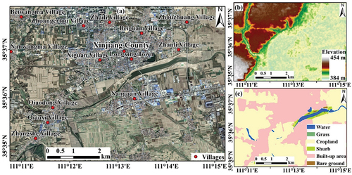
With a total length of 713 km and a basin area of 39,721 km², the Fen River is the second-largest tributary of the Yellow River and the largest river in Shaanxi Province of China. We focused our research on a 1-in-30-year flood event that took place in the Autumn 2021 along the Fen River and led to large-scale floods in Xinjiang County. The flood started at about 17:00 on October 7 affected by heavy rainfall and upstream water, and the embankment in the northern section of the Fen River broke with a length of nearly 20 m. About 20,000 people were urgently evacuated.

2.2. Data

We used 88 Sentinel-1 GRD images (Table 1) to study the dynamic process of the flood. A total of 84 images from 1 January 2020 to 30 September 2021 were used to generate a reference background before the flood and the other four images, sampled at different stages during the flood process, were used to detect any changes caused by the flood. As shown in Figure 2, the flooded areas exhibited as dark pixels with very low backscatter coefficient, and we can clearly see that the most serious flood-spreads occurred on or near 12 October 2021.

Figure 2. Sentinel-1 GRD images of the flood process. (a) 2021-10-05. (b) 2021-10-12. (c) 2021-10-17. (d) 2021-10-24. Dark color represents low backscatter coefficients whilst bright color represents high backscatter coefficients. The white box in (b) is used in Figure 7.

Table 1. Sentinel-1 GRD data.

Flood stage	Acquisition	No. of images	Mode	Orbit direction	Polarization	Spatial resolution
Non-flood	1 January 2020 to 30 September 2021	84	IW	ascending	VV	10 × 10m
Emergence	5 October 2021	1	IW	ascending	VV	10 × 10m
Peak	12 October 2021	1	IW	ascending	VV	10 × 10m
Receding	17 October 2021	1	IW	ascending	VV	10 × 10m
Disappearance	24 October 2021	1	IW	ascending	VV	10 × 10m

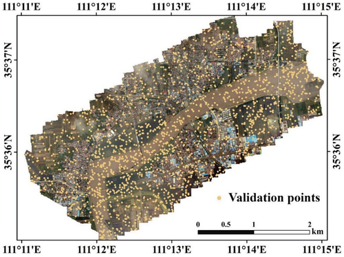
A 0.1 m spatial resolution Digital Orthophoto Map (DOM) imaged by Unmanned Aerial Vehicle (UAV) (Figure 3) was acquired in the morning of 12 October 2021 during the flood, the same date with one of the Sentinel-1 GRD images as shown in Table 1. This UAV image was then used for validation. We used the Agisoft Photoscan software to process the UAV DOM by adding and aligning photos, building dense clouds, meshing, and matching (Liu et al. 2018).

Figure 3. The UAV DOM obtained on 12 October 2021. Yellow points were randomly generated (2,000 in total) for validation purposes in Section 4.

3. Methods

3.1. Sentinel-1 GRD data processing

Due to its wide coverage and high spatial resolution, processing SAR image time series is generally time-consuming, which hinders their applications in rapid flood responses. To solve this, the Google Earth Engine (GEE) platform published by Google was used. GEE supports the development of global-scale data products using satellite image time series by online programming (Gorelick et al. 2017). This avoids the time-consuming process of data downloading and preprocessing. The GEE cloud platform has a complete and constantly updated Sentinel-1 GRD dataset which provides a great opportunity for wide-area, dynamic, and long-term flood monitoring research (DeVries et al. 2020; Tamiminia et al. 2020).

The Sentinel-1 SAR dataset released by GEE includes Sentinel-1 GRD data collected in extra wide-swath (EW), interferometric wide-swatch (IW), and strip map (SM) modes, which are preprocessed using tools provided by the ESA Sentinel Application Platform (SNAP) software package. In our experiment, the IW GRD image was used. The GEE platform first applied the orbital file to control the geometric accuracy within 5 cm (Prats-Iraola et al. 2015). Second, the thermal noise of all GRD images collected after 12 January 2018 was removed, which was mainly related to the edge of the image band (Ali et al. 2018). Radiometric calibration was carried out to produce a unitless backscatter intensity (${\sigma }_{\mathit{int}}$) (Sabel et al. 2012). Terrain geocoding was used to encode images using SRTM DEM (Farr et al. 2007). Finally, according to Equation 1, the backscatter intensity was converted to the backscatter coefficient (${\sigma }^0$) measured in decibels (dB) (Lin et al. 2019). All images were projected to the WGS84 system.

(1) ${\sigma }^0=10\mathit{lo}{g}_{10}{\sigma }_{\mathit{int}}$(1)

3.2. Pareto scaling normalization

As a first step in deriving a probabilistic flood map, PS normalization is used to acquire the flood anomaly information so that a reference background for the non-flood period can be established.

First, we calculated the multi-temporal mean (${\mu }_{nf}^x$) and standard deviation ($s_{nf}^x$) for each pixel of the 84 images before the flood (Figure 4(a,b)), where the subscript nf represented the non-flood period. ${\sigma }_{i,x}^0$ represents the observed pixel backscatter coefficient in the i_th image at pixel x:

Figure 4. PS normalization of the GRD images during the flood process. (a) Mean backscatter coefficients for the historical reference background from 2020-01-01 to 2021-09-30. (b) The square root of the standard deviation of backscatter coefficients for the same period as (a). (c-f) PS normalization for images 2021-10-05, 2021-10-12, 2021-10-17 and 2021-10-24, respectively.

(2) ${\mu }_{nf}^x=\frac{{\sum }_{i=1}^n{\sigma }_{i,x}^0}{\mathit{n}}{s}_{nf}^x=\sqrt{\frac{{\sum }_{i=1}^n{\left({\sigma }_{i,x}^0-{\mu }_{nf}^x\right)}^2}{\mathit{n}-1}}\mathit{n}=84$(2)

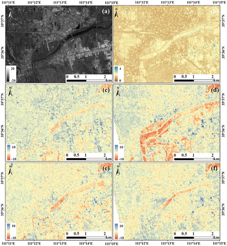
Second, we normalized the backscatter coefficient of pixel x during the flood using Equation 3, where t is the acquisition time of the image.

(3) $\widetilde{{\sigma }_{t,x}^0}=\frac{{\sigma }_{t,x}^0-{\mu }_{nf}^x}{\sqrt{s_{nf}^x}}$(3)

In order to better represent the background information of pixels, it is required that the sensor acquisition mode IW, EW, SM, and wave (WV), orbital direction (ascending and descending) and polarization mode (VV or VH) of multi-phase image data should be consistent. The normalization result is shown in Figure 4. It is clear that the PS normalization of the event images can well represent the anomaly degree of the flood event images from the background information.

3.3. Bayesian flood probability estimation

The flood probability estimation algorithm depends on the statistical distribution assumption and Bayesian inference (Giustarini et al. 2016; Schlaffer et al. 2017). Pixels on the PS normalized image are regarded as disjoint union data of flooded (F) and non-flooded ($\bar{F}$) parts (Chini et al. 2016), and the probability of each pixel being flooded is calculated according to the normalized backscatter value. The probability density function of the backscatter coefficient distribution of flooded pixels is $\mathit{p}\left({\sigma }^0|\mathit{F}\right)$, and that of non-flooded pixels is $\mathit{p}\left({\sigma }^0|\bar{F}\right)$. The marginal distribution of the normalized backscatter coefficient is $\mathit{p}\left({\sigma }^0\right)$, which can be expressed as Equation 4, where $\mathit{p}\left(\mathit{F}\right)+\mathit{p}\left(\bar{F}\right)=1$.

(4) $\mathit{p}\left({\sigma }^0\right)=\mathit{p}\left({\sigma }^0|\mathit{F}\right)\mathit{p}\left(\mathit{F}\right)+\mathit{p}\left({\sigma }^0|\bar{F}\right)\mathit{p}\left(\bar{F}\right)$(4)

When the normalized backscatter coefficient ${\sigma }^0$ of a pixel is given, the conditional probability of pixel inundation is estimated by using Bayesian inference as follows:

(5) $\mathit{p}\left(\mathit{F}|{\sigma }^0\right)=\frac{p\left({\sigma }^0|\mathit{F}\right)\mathit{p}\left(\mathit{F}\right)}{\mathit{p}\left({\sigma }^0\right)}$(5)

By substituting the Equation 4 into the Equation 5, we can further obtain Equation 6 for calculating $\mathit{p}\left(\mathit{F}|{\sigma }^0\right)$.

(6) $\mathit{p}\left(\mathit{F}|{\sigma }^0\right)=\frac{p\left({\sigma }^0|\mathit{F}\right)\mathit{p}\left(\mathit{F}\right)}{\mathit{p}\left({\sigma }^0|\mathit{F}\right)\mathit{p}\left(\mathit{F}\right)+\mathit{p}\left({\sigma }^0|\bar{F}\right)\mathit{p}\left(\bar{F}\right)}$(6)

In the above equation, it is necessary to estimate $\mathit{p}\left(\mathit{F}\right)$, $\mathit{p}\left(\bar{F}\right)$ $\mathit{p}\left({\sigma }^0|\mathit{F}\right)$, and $\mathit{p}\left({\sigma }^0|\bar{F}\right)$, respectively. $\mathit{p}\left(\mathit{F}\right)$ and $\mathit{p}\left(\bar{F}\right)$ denote a priori probability, which refer to the probability that pixels are classified as flooded or non-flooded according to existing studies (e.g. Meng et al. 2019). In this paper, we chose the default value of a priori probability $\mathit{p}\left(\mathit{F}\right)$ and $\mathit{p}\left(\bar{F}\right)$ to 0.5 according to Westerhoff et al. (2013). A larger or a smaller $\mathit{p}\left(\mathit{F}\right)$ means the initial probability assigned to the hypothesis is either leaning toward the occurrence of the flood or vice versa.

Because of its specular reflection, the flood water body shows a low backscatter coefficient in Sentinel-1 GRD images, and the statistical distribution histogram of backscatter coefficient $\mathit{h}\left({\sigma }^0\right)$ of images with a certain range of flood water body is one bimodal as a whole. In fact, previous studies have shown that the logarithmic variation of the SAR intensity data obeys a Gaussian distribution (Xie et al. 2002). In other words, $\mathit{h}\left({\sigma }^0\right)$ can be used to calculate the conditional probability distribution of $\mathit{p}\left({\sigma }^0|\mathit{F}\right)$ and $\mathit{p}\left({\sigma }^0|\bar{F}\right)$. In this paper, we assumed that the statistical distribution histogram of the flooded pixels and the non-flooded pixels obeyed Gaussian distribution. At a given normalized backscatter coefficient value, the conditional probability distributions $\mathit{p}\left({\sigma }^0|\mathit{F}\right)$ and $\mathit{p}\left({\sigma }^0|\bar{F}\right)$ can be expressed as follows:

(7) $\mathit{p}\left({\sigma }^0|\mathit{F}\right)=\frac{1}{s_F\sqrt{2\mathit{\pi }}}{e}^{-\frac{{\left({\sigma }^0-m_F\right)}^2}{2s_F^2}}$(7)

(8) $\mathit{p}\left({\sigma }^0|\bar{F}\right)=\frac{1}{s_{\bar{F}}\sqrt{2\mathit{\pi }}}{e}^{-\frac{{\left({\sigma }^0-m_{\bar{F}}\right)}^2}{2s_{\bar{F}}^2}}$(8)

The estimation of the four unknown parameters in the above equation ($m_F$, $s_F$, $m_{\bar{F}}$, $s_{\bar{F}}$) was mainly through the application of the hybrid modeling technique to the image histogram $\mathit{h}\left({\sigma }^0\right)$. This was achieved by iteratively fitting the histogram to the Gaussian distribution by,

(9) $\mathit{h}\left({\sigma }^0\right)=\underset{\mathrm{flooded}\mathrm{pixels}}{A_F{e}^{-\frac{{\left({\sigma }^0-m_F\right)}^2}{2s_F^2}}}+\underset{\mathrm{non}-\mathrm{flooded}\mathrm{pixels}}{A_{\bar{F}}{e}^{-\frac{{\left({\sigma }^0-m_{\bar{F}}\right)}^2}{2s_{\bar{F}}^2}}}$(9)

where $A_F$ and $A_{\bar{F}}$ represent the peaks of flooded and non-flooded pixels in the histogram (Wilks 2006), respectively. The initial values of the six parameters ($A_F$, $A_{\bar{F}}$ $m_F$, $s_F$, $m_{\bar{F}}$, $s_{\bar{F}}$) were obtained by using the Otsu algorithm (Otsu 1979).

The main steps included the selection of the region of interest (ROI) and the determination of the classification threshold. The selected ROI had a bimodal distribution, and the threshold was determined by traversing the intensity values from the smallest to the largest so that the interclass variance was maximized. Through the threshold, the ROI can be divided into two classes, and Gaussian fitting was performed separately to obtain the initial values of the six parameters. Then, the Levenberg-Marquardt algorithm was used for nonlinear least square fitting (Marquardt 1963), and the optimal distribution parameters are obtained by iterative calculations, until the four parameters converge.

When the four parameters ($m_F$, $s_F$, $m_{\bar{F}}$, $s_{\bar{F}}$) were determined, we can get the conditional probability distributions of $\mathit{p}\left({\sigma }^0|\mathit{F}\right)$ and $\mathit{p}\left({\sigma }^0|\bar{F}\right)$ using Equation 7(7) $\mathit{p}\left({\sigma }^0|\mathit{F}\right)=\frac{1}{s_F\sqrt{2\mathit{\pi }}}{e}^{-\frac{{\left({\sigma }^0-m_F\right)}^2}{2s_F^2}}$(7) and 8(8) $\mathit{p}\left({\sigma }^0|\bar{F}\right)=\frac{1}{s_{\bar{F}}\sqrt{2\mathit{\pi }}}{e}^{-\frac{{\left({\sigma }^0-m_{\bar{F}}\right)}^2}{2s_{\bar{F}}^2}}$(8) . The probability $\mathit{p}\left(\mathit{F}|{\sigma }^0\right)$ for each pixel after a given normalized backscatter coefficient can be calculated from Equation 6(6) $\mathit{p}\left(\mathit{F}|{\sigma }^0\right)=\frac{p\left({\sigma }^0|\mathit{F}\right)\mathit{p}\left(\mathit{F}\right)}{\mathit{p}\left({\sigma }^0|\mathit{F}\right)\mathit{p}\left(\mathit{F}\right)+\mathit{p}\left({\sigma }^0|\bar{F}\right)\mathit{p}\left(\bar{F}\right)}$(6) . The method flow includes data preparation, PS normalization, Bayesian probability estimation, and probabilistic flood mapping, which are shown in Figure 5.

Figure 5. The improved flood probability mapping based on PS and Bayesian framework.

3.4. The reliability diagram validation method

To validate the obtained probabilistic flood maps, we used high-resolution UAV DOM as ground truth obtained on the same date (12 October 2021) with the GRD image. To quantitatively calculate the accuracy statistics, 2,000 pixels covering the entire DOM were randomly selected (Figure 3) with their flooding status (flooded or non-flooded) being manually labeled.

We used a reliability diagram method proposed by Horritt (2006) to evaluate the performance of probabilistic flood mapping. The reliability diagram uses the calibration function to validate the flood probability map. First, the range of probability values [0, 1] is split into N = 10 intervals (Brocker and Smith 2007; Hostache et al. 2011; Renard and Lall 2014), i.e. I_k∈{[0, 0.1], (0.1, 0.2], … , (0.9, 1]}, with centers i_k = 0.05, 0.15, … , 0.95, k = 1, 2, … , N. The values of these centers represent an averaged flood probability of the pixels within each interval (i.e. modeled probability). Second, the value of the calibration function for each interval is calculated as the proportion (${\bar{Q}}_{\mathit{k}}$) of the pixels in the interval that are actually observed by the DOMs as flooded (i.e. the observed probability). This observed probability should be close to the modeled probability if the calculated flood probability maps successfully represent the real world.

We used the “degree” of reliability to quantitatively assess the accuracy of the flood probability maps,

(10) $R_e=\sqrt{\frac{{\sum }_{k=1}^N{\left(i_k-{\bar{Q}}_{\mathit{k}}\right)}^2{n}_k}{{\sum }_{k=1}^N{n}_k}}$(10)

where$n_k$ is the total number of pixels in each interval. Re is given in the form of weighted root-mean-square error, which indicates the degree of deviation between the i_k and ${\bar{Q}}_{\mathit{k}}$. Small Re indicates a higher accuracy of the probabilistic flood map and vice versa.

3.5. Additional methods used for comparisons

To compare the proposed method with other methods, we also obtained flood delineation results from two methods as mentioned in Section 1, including the Sentinel-1 dual-polarized water index (SDWI) threshold method (J. Guo et al. 2021) and the Z-score method (DeVries et al. 2020).

(1) SDWI

By leveraging the distinctive signal contrast between water and other elements within dual-polarized bands, SDWI effectively amplifies water body details while concurrently mitigates the impact of soil and vegetation interference (Tian et al. 2022). SDWI can be computed as follows:

(11) $\mathit{SDWI}=ln\left(10\times \mathit{VV}\times \mathit{VH}\right)-8$(11)

Where VV and VH are values of the dual-polarized in polarization mode, respectively.

(2) Z-score

This approach employs temporal anomaly measures for flood monitoring. The temporal mean backscatter coefficient (${\bar{\omega }}_0$) and standard deviation backscatter coefficient ($\mathit{std}\left({\omega }_0\right)$) are computed during the non-flood period. For each observation captured at time q, the backscatter Z-score is determined based on Equation 12, with consideration given to the polarization mode (p), sensor acquisition mode(s), and orbital direction (d).

(12) $Z_{sc\mathrm{ore}}^{p,s,d}\left(\mathit{q}\right)=\frac{{\omega }_0^{p,s,d}\left(\mathit{q}\right)-{\bar{\omega }}_0^{\mathit{p},\mathrm{s},\mathit{d}}}{\mathit{std}\left({\omega }_0^{p,\mathrm{s},d}\right)}$(12)

We selected the image on 12 October 2021 (the most flood-affected image) in the study area as the comparison image and generated binary flood maps, respectively, by the SDWI and Z-score methods. We first calculated the SDWI and the threshold (−0.06) was obtained from the histogram of the SDWI to extract the flooded pixels (Tian et al. 2022). For the Z-score method, we tested a set of thresholds (−1.50, −1.00, and −0.50) and obtained overall agreements of 0.76, 0.79, 0.78, respectively. Therefore, the optimal threshold was determined as −1.00 (DeVries et al. 2020).

As the assessment method in Section 3.4 is used for probability maps and is not suitable to evaluate binary maps, we used additional accuracy indicators including the user’s accuracy, producer’s accuracy (UA and PA), overall accuracy (OA), and Kappa coefficient (Congalton 1991; Thompson and Walter 1988). Higher UA and PA values indicate smaller numbers of overpredicted pixels and underpredicted pixels, respectively. OA determines the overall efficiency of an algorithm, representing the proportion of correctly classified samples to all samples. Kappa indicates the degree of consistency between the real data on the ground and the classification value, with a value closer to 1 suggesting better consistency in the classification result.

4. Results

4.1. Flood probability maps

The generated flood probability maps of the four dates during the flood process (Table 1) are shown in Figure 6. The whole process from occurrence to disappearance of the Xinjiang flood was captured. Affected by heavy rainfall, the cultivated crops in a small part of Figure 6(a) were submerged on October 5th (denoted as a red box). On October 7th, the dam in the north section of Fen River near Qiaodong Village collapsed (the red box in Figure 6(b)). At the same time, several days of rainfall made the inundation range in the study area reach the maximum on October 12th, as shown in Figure 6(b). Most of the cultivated crops (see Figure 1(c)) around the original water had been submerged, presenting a flaky area. On the same day, the flood water overflowed into Nanguan Village near the river, and the local residents were evacuated. Figure 6(c) shows that the flood in a large area of cultivated crops and the ponding in Nanguan Village (red boxes) were also gradually receding on October 17th. In Figure 6(d), the flooded areas had diminished, and the flood in the cultivated crops had largely receded.

Figure 6. The flood probability maps. (a) 2021-10-05, (b) 2021-10-12, (c) 2021-10-17, (d) 2021-10-24. (e) Four flood stages identified by the percentage of flooded pixels with a flood probability of larger than 0.8.

The flood probability maps capture the dynamic process of flood progression. As discussed by Rahman and Thakur (2018) and H. Yang et al. (2021), the lifecycle of a flood can be divided into different stages depending on the spatial coverage of the flooded areas. By calculating the percentage of flooded pixels whose probabilities are greater than 0.8, we distinguished four stages during the flood process, i.e. emergence, peak, receding, and disappearance (Figure 6(e)). During the emergence stage, the flood waters began to accumulate and spread across the affected area (Figure 6(a)). This initial phase was characterized by the rising water levels and the encroachment of flood waters into low-lying regions. As the flood continued to intensify, it reached its peak stage, with the flood probability map (Figure 6(b)) precisely delineated the regions most susceptible to severe flooding. This marked the period when the flood waters attained their highest levels, causing significant inundation of the surrounding terrain. Following the peak stage, the inundation area decreased gradually during the receding stage. The map (Figure 6(c)) tracked and visualized the gradual reduction in water levels, aiding in the assessment of potential risks and facilitating recovery efforts. Finally, the disappearance stage (Figure 6(d)) marked the point at which the flood waters dramatically subsided, and most affected areas returned to their normal state.

By capturing these four stages of the flood process, the flood probability maps play a crucial role in understanding the temporal evolution and spatial distribution of the flood event. These identified characteristics serve to enhance our flood response capabilities. For example, images at different flood stages will be obtained during a flood event so that we can analyze the spatial characteristics of the flood-affected pixels to determine the flood status and evolution over time.

4.2. Validation of flood probability maps

To validate the performance of the proposed method, we selected a ROI (the white box in Figure 2) to check the distinguishability of flooded and non-flooded pixels. The validation results are shown in Figure 7 (the first three rows). To highlight the importance of the PS normalization, we show here the validation results of both the non-normalized and normalized images. The backscatter coefficient histogram $\mathit{h}\left({\sigma }^0\right)$ of the 12 October 2022 image (Figures 7(a1) and (b1)) can be well fitted by two Gaussian curves using the Levenberg-Marquardt nonlinear least square fitting, respectively, for the flooded (red) and non-flooded (green) parts, with the normalized image having two obvious peaks which are easier to be separated into two categories. Figures 7(a2) and (b2) show that the marginal distribution function of ${\sigma }^0$ derived by substituting four parameters ($m_F$, $s_F$, $m_{\bar{F}}$, $s_{\bar{F}}$) into Equation 7(7) $\mathit{p}\left({\sigma }^0|\mathit{F}\right)=\frac{1}{s_F\sqrt{2\mathit{\pi }}}{e}^{-\frac{{\left({\sigma }^0-m_F\right)}^2}{2s_F^2}}$(7) and 8(8) $\mathit{p}\left({\sigma }^0|\bar{F}\right)=\frac{1}{s_{\bar{F}}\sqrt{2\mathit{\pi }}}{e}^{-\frac{{\left({\sigma }^0-m_{\bar{F}}\right)}^2}{2s_{\bar{F}}^2}}$(8) from which the flooded condition probability $\mathit{p}\left(\mathit{F}|{\sigma }^0\right)$ was calculated based on Bayesian estimation (Equation 6(6) $\mathit{p}\left(\mathit{F}|{\sigma }^0\right)=\frac{p\left({\sigma }^0|\mathit{F}\right)\mathit{p}\left(\mathit{F}\right)}{\mathit{p}\left({\sigma }^0|\mathit{F}\right)\mathit{p}\left(\mathit{F}\right)+\mathit{p}\left({\sigma }^0|\bar{F}\right)\mathit{p}\left(\bar{F}\right)}$(6) ). The difference between non-normalized and normalized images lied in their pixel value range and representation. The former might have different pixel value ranges across different images, requiring additional preprocessing when comparing and processing them. However, the latter provided better data consistency and processing capabilities by standardizing the pixel values to a unified range. After applying PS normalization, the boundary between flooded and non-flooded became clear and hence easier to distinguish.

Figure 7. The evaluation of the flood probability maps respectively for the non-normalized (a) and normalized (b) results. The first row shows the backscatter histogram Gaussian curve fitting of the ROI defined in Figure 2 (the white box). The second row shows the marginal distribution of the backscatter coefficient of the same ROI. The third row shows the probability of a pixel being flooded of the same ROI based on the Bayesian estimation Equation 5(5) $\mathit{p}\left(\mathit{F}|{\sigma }^0\right)=\frac{p\left({\sigma }^0|\mathit{F}\right)\mathit{p}\left(\mathit{F}\right)}{\mathit{p}\left({\sigma }^0\right)}$(5) . The fourth row shows the reliability diagrams using the 2000 random validation samples on the UAV image.

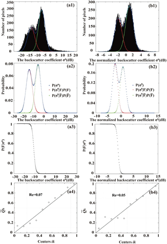
We then used a high-resolution UAV DOM and the reliability diagram as mentioned in Section 3.4 to validate the accuracy of the flood probability map. Since the DOM was captured on October 12, we used the flood probability map on the same date to avoid any uncertainties caused by time differences. We sampled 2,000 random points in Figure 3 whose flooding status (flooded or non-flooded) was identified by manual interpretation. The reliability diagrams (Re) in Figures 7(a4) and 7(b4) represent the consistency between the flood probability map and 2,000 verification points on the high-resolution DOM. It can be observed that the accuracies of the flood probability maps of both methods were relatively low when the pixel’s probability of being flooded was small (<0.5). This was because within this range, the backscatter characteristics of the pixels were not predominantly influenced by water but exhibited complex features. However, as the flood probability increased and exceeded 0.5, the accuracies improved significantly. The accuracy of the normalized method was notably enhanced when the pixel’s probability of being flooded was large (>0.5), suggesting it aided in improving the accuracy of flood detection for pixels with a higher probability of being flooded. The overall reliability (measured by Equation 10(10) $R_e=\sqrt{\frac{{\sum }_{k=1}^N{\left(i_k-{\bar{Q}}_{\mathit{k}}\right)}^2{n}_k}{{\sum }_{k=1}^N{n}_k}}$(10) ) of the normalized result reached 0.05, improved by 28.57% compared with the non-normalized result, indicating an improvement in the accuracy and consistency of the flood probability maps. Detailed statistics are shown in Table 2.

Table 2. Detailed data information for reliability diagrams.

Probability	Probability level	Percentage of flooded pixels by modelling ($i_k)$(%)	Non-normalized	PS normalized
			Percentage of flooded pixels by UAV (${\bar{Q}}_{\mathit{k}})$(%)	Percentage of flooded pixels by UAV (${\bar{Q}}_{\mathit{k}})$ (%)
0.0–0.1	Low	5	14	9
0.1–0.2		15	13	32
0.2–0.3		25	19	28
0.3–0.4		35	25	30
0.4–0.5	Medium	45	47	29
0.5–0.6		55	61	58
0.6–0.7	High	65	70	67
0.7–0.8		75	76	74
0.8–0.9	Extremely-high	85	91	84
0.9–1.0		95	98	94
Re	–	–	0.07	0.05

4.3. Comparisons against SDWI and Z-score

The flood maps, respectively, from this paper, SDWI and Z-score methods are shown in Figure 8. The flood probability map was converted into a binary map by a given threshold of 0.4 (medium to extremely high flood probabilities as will be discussed in Section 5.1). The resultant statistics are listed in Table 3. The number of pixels in the flooded and non-flooded columns represent actual categories from the high-resolution DOM, and the corresponding columns represent classified categories according to different methods. The SDWI method achieved a high UA, hovering around 87%; however, its PA was slightly lower, standing at approximately 75%, compared to the Z-score method (78%). Our proposed method yielded promising results, achieving the highest OA at 85.20% compared to 82.30% and 79.35% from the other two methods, respectively, signifying its comparative effectiveness. The Kappa coefficient was 0.70 for our method, which was considerably higher than the other two methods, suggesting a notably high level of consistency between the flood classification presented in this paper and the ground truth data.

Figure 8. The flood binary maps generated, respectively, by this paper (a), SDWI (b) and Z-score(c).

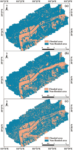
Table 3. Accuracy assessment of flooded and non-flooded classification using different methods.

Method		Flooded	Non-flooded	PA(%)	UA(%)	OA(%)	Kappa
This paper	Flooded	793	186	81.00	87.82	85.20	0.70
	Non-flooded	110	911	89.23	83.04
SDWI	Flooded	731	248	74.67	87.34	82.30	0.64
	Non-flooded	106	915	89.62	78.68
Z-score	Flooded	761	218	77.73	79.60	79.35	0.59
	Non-flooded	195	826	80.90	79.11

The predominant land use types in the study area are comprised of croplands and built-up areas, accounting for a total of 93.1% of the entire area. Table 4 presents a comparison of the flood mapping results, respectively, on croplands and built-up areas using different methods. Our proposed method demonstrated improved performance when compared to both SDWI and Z-score, particularly noticeable in the reduction of the false-negative samples and false-positive samples across different land use types. On croplands, our method outperformed the SDWI method by reducing the false-negative samples by ~3.4% and lowering the false-positive samples by 1.7%. When compared with the Z-score, our method only exhibited a slight improvement in false-negative reduction (0.9%), but a more substantial false-positive decrease (50%). The improvements were more obvious in built-up areas, with the proposed method displaying a dramatic decline in the false-negative samples (61.2% and 17.4% decreases compared to SDWI and Z-score, respectively). The false-positive samples also decreased from 118 and 171, respectively, for SDWI and Z-score to 98 for the new method. In conclusion, the method introduced in this study consistently improves the accuracy of flood mapping, especially demonstrating a marked advantage in minimizing false-negative samples, and therefore enhances the overall classification accuracy.

Table 4. Flood mapping results among different land use types (no. of points).

Land use		This paper	SDWI	Z-score
Cropland	True positive	613	554	602
	False positive	10	12	20
	True negative	269	267	259
	False negative	115	174	126
Built-up area	True positive	76	46	72
	False positive	98	118	171
	True negative	620	600	547
	False negative	19	49	23

The observed performance differences in different land use types can primarily be attributed to their significant differences in surface characteristics. Croplands generally facilitate accurate flood detection due to their uniform surface reflectance properties whereas built-up areas show complex reflection patterns (e.g. shadow effects) which complicate flood recognition tasks (Pulvirenti et al. 2016). It is therefore suggested that the land use type should be carefully considered when assessing flood mapping results.

5. Discussion

5.1. The dynamic process of flooding

Previous studies distinguished flooded and non-flooded areas by setting a threshold probability value 0.5 based on the probability map. But, this paper divided the flood probability interval into four levels (Table 2), namely extremely high (0.8–1.0), high (0.6–0.8), medium (0.4–0.6), and low (0.0–0.4) to analysis the flood process in detail. These probability breaks were set according to the temporal and spatial characteristics of the flood probability maps. Various algorithms have used probability breaks to analyze probability maps, including natural breaks (Tien Bui et al. 2019), quantile breaks (Rosser, Leibovici, and Jackson 2017; Tehrany et al. 2015), and customized breaks (Alfonso, Mukolwe, and Di Baldassarre 2016). Natural breaks can reveal the inherent structure and patterns in data but may lead to pixels in critical areas being incorrectly assigned to a higher flood probability level when the distribution of flood probabilities is non-continuous and uneven. Quantile breaks ensure a uniform distribution of probability values within each category so that they are not suitable when flood probability distributions are irregular, e.g. fluctuations near lower quantiles can potentially result in some pixels being inappropriately categorized into a higher risk tier. In this study, we used a customized classification method to deal with the dynamic process of flooding. This approach allows us to flexibly set thresholds based on the physical characteristics of floods and their actual impacts, thus enabling a more precise representation of the spatial distribution (Figure 6) and temporal evolution (Figure 9) of pixels affected by floods.

Figure 9. Four levels of flood probabilities and their transformation during the flood from 2021-10-05 to 2021-10-24.

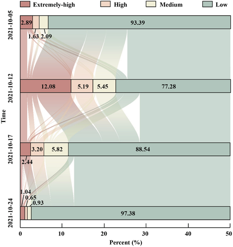
The extremely high level represented a significant change in ground reflectivity caused by the flood, where the corresponding land use/cover was completely submerged. The high level signified a considerable change in reflectivity, indicating a semi-submerged state of the ground. For instance, in vegetated areas, the degree of inundation might be approximately half. The medium level indicated a moderate change in reflectivity, and pixels assigned to this level mostly represented areas in a transitional state. Continuous rainfall accumulation or drainage system blockage might result in localized floods in these areas. On the other hand, the low level denoted relatively stable reflectivity, with minimal submergence. This included permanent water bodies or high-rise buildings that remained largely unaffected by the flood.

To explore the dynamic process of flooding, we conducted statistical calculations to analyze the temporal evolution of flood-affected pixels at each of the four flood probability levels. The results are illustrated in Figure 9, revealing distinct temporal characteristics for different flood levels. Starting from October 12th, the area transitioning from the extremely high level to other levels was considerably larger than the area transitioning from other levels to the extremely high level. This indicated a sharp and relatively short-lived peak in flooding. By October 17th, the high and medium levels experienced transitions not only from the extremely high level but also from the low level. Notably, the area occupied by medium-level pixels remained relatively unchanged. In the final stage, pixels sequentially shifted from medium to extremely high levels, with the majority ultimately transitioning to the lower level. Comparing the three levels excluding the low level, the duration of their peaks varied significantly, with the medium level exhibiting the longest duration and the extremely high level the shortest.

During the early stages of flooding, areas within extremely high and high levels are typically the first to be affected because they are often located in low-lying areas that are prone to flooding. As the flood began to recede, the water level in these areas decreases, causing the backscatter coefficient of pixel changes significantly, and the pixel probability values decrease. Such a detailed quantitative analysis of the dynamic evolution of the flood process combining spatial (Figure 6) and temporal (Figure 9) information would illustrate flood risk effectively and is of great importance in decision-making.

5.2. Method transferability

In order to examine the transferability of the method, we added another three testing sites including the River Severn in the city of Tewkesbury, UK (11 February 2016), a hurricane Harvey-related flood event in the metropolitan area of Houston, USA (30 August 2017), and the Webi Shebelle River in the city of Beledweyne, Somalia (7 May 2018). We first examined the consistency of the proposed method by calculating the normalized backscatter coefficient and an optimal coefficient that should show a two-peak distribution which makes the flood-affected pixels more distinguishable. In the absence of high-precision ground truth data, we further compared the resultant flood maps against those extracted through NDWI (McFeeters 1996) analysis on Sentinel-2 optical images captured during the flood event (respectively, on 10 February 2016 and 4 September 2017, Figures 10(a3) and (b3)). For the third event where the cloud coverage was high, we used the flood extent map provided by UNITAR (https://unitar.org/unosat/node/44/2796) which was manually extracted using Radarsat-2 data collected on 9 May 2018.

Figure 10. The first row shows the original sentinel-1 GRD images. The second row shows the flood probability maps generated by the proposed method. The third row shows the flood extent map generated by optical images (the first two columns) and SAR image (the third column). The fourth row shows the marginal distribution of the normalized backscatter coefficient. (a) Tewkesbury, (b) Houston (USA), (c) Beledweyne.

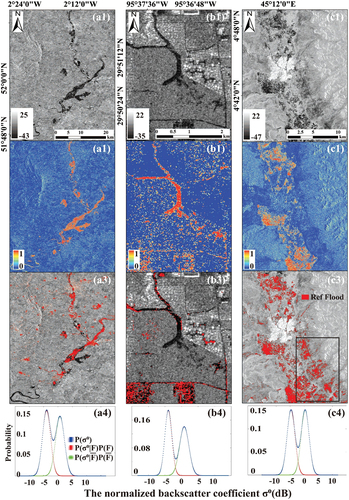
The resultant flood probability maps are shown in Figure 10. The normalized backscatter coefficients used in the proposed method for the three events showed apparent two-peak distributions which facilitated the identification of flooded pixels. The proposed method well captured the spatial characteristics of the flood-affected areas which showed a high consistency with the referenced flood maps (third row in Figure 10). One notable difference occurred in the black box (Figure 10(c3)) where numerous points were classified as flooded in UNITAR but not by our proposed method. However, Martinis, Plank, and Ćwik (2018) have found that this particular area exhibited a unique and stable characteristic of low backscatter, maintaining values around approximately −20 dB, so that it was not caused by flooding. Our proposed method overcame this problem by considering historic images in the PS normalization step. However, it is difficult to calculate precise statistics between our flood probability maps and the reference maps as i) differences in acquisition times can lead to shifts in the actual extent of flooding; and ii) the presence of clouds can obstruct clear depiction of the true flood conditions in optical images. To conclude, the proposed method exhibits a high degree of transferability which underscores the method’s robustness and its capability to deliver commendable performance in a wide array of contexts and applications.

Nonetheless, flood probability maps still exhibit limitations in specific environments, particularly in areas characterized by dense vegetation and pronounced shadow effects, and some edges of flat anthropogenic structures within cities can be misinterpreted as water due to layover (Giustarini et al. 2013). These complexities can contribute to inaccuracies in pinpointing the boundaries of flood zones and estimating the full extent of impacted areas. Despite these challenges, flood mapping using SAR images acts as a significant supplement to traditional flood mapping methods. By consistently refining and enhancing the methodologies employed in flood probability mapping, there exists a potential to improve the precision and dependability of flood monitoring and associated geographical information extraction procedures.

6. Conclusion

In this study, we introduced a novel flood mapping approach that combined PS normalization and Bayesian probability estimation. The utilization of image normalization allowed for a distinct differentiation between flooded and non-flooded pixels within the image. The results revealed a remarkable improvement of 28.57% in reliability compared to the non-normalized method and exhibited a high level of agreement, with a 95% match to the high-resolution UAV DOM. Compared with SDWI and Z-score methods, the new method generated satisfying results with the highest UA and PA (above 88% and 81%). This enhancement indicated that the probability map generated through our proposed approach exhibited high accuracy and feasibility. By combining Gaussian fitting and Bayesian probability calculations, the proposed method aims to make the flood mapping process more adaptable and less reliant on manually set thresholds.

Previous research primarily concentrated on examining the extent of flood inundation during specific flood events, with limited studies focusing on monitoring the dynamics of floods over time. This paper aims to address this gap by acquiring four probability maps that capture various stages of the flood process, enabling the monitoring of flood dynamics. We divided the flood probability range of [0, 1] into four levels: extremely high, high, medium, and low. Each probability level exhibited unique temporal characteristics, with the extremely high level experiencing rapid increases and decreases, while the medium level displaying more gradual changes. By observing these variations, we gained insights into the dynamic nature of flood events beyond mere inundation mapping.

The findings from this study have significant implications for the development of comprehensive flood risk management strategies. By incorporating this method into existing flood management practices, authorities and stakeholders can enhance their ability to minimize the adverse impacts of floods on communities, infrastructure, and the environment. In the future work, we will explore the integration of additional remote sensing data sources, such as multispectral or hyperspectral images, to enhance the method’s accuracy and reliability. Combining data from different sources (e.g. crowdsourced data or social media information) can provide a more comprehensive understanding of flood dynamics so that a more precise and efficient flood response plan can be made.

Acknowledgments

The research was funded in part by the National Key Research and Development Program of China under Grant 2020YFC1512000, in part by the Shaanxi Province Science and Technology Innovation Team under Grant 2021TD-51, in part by the Shaanxi Province Geoscience Big Data and Geohazard Prevention Innovation Team (2022), and in part by the Fundamental Research Funds for the Central Universities, Chang’an University, China under Grant 300102263401, 300102260301, 300102262902, 300102264901 and 300103724057.

Disclosure statement

No potential conflict of interest was reported by the author(s).

Data availability statement

The Sentinel-1 GRD datasets were freely provided by Google Earth Engine (“COPERNICUS/S1_GRD,” path 11 and 113) on https://code.earthengine.google.com/ (accessed on 12 April 2023). The ALOS digital elevation model (DEM) with can be found at https://search.asf.alaska.edu/#/ (accessed on 12 April 2023). Land use/cover dataset was provided by ESRI and downloaded from https://www.arcgis.com/apps/instant/media/index.html?appid=fc92d38533d440078f17678ebc20e8e2 (accessed on 12 April 2023).

Additional information

Funding

The work was supported by the Fundamental Research Funds for the Central Universities, Chang’an University, China [300102260301; 300102262902]; Fundamental Research Funds for the Central Universities, Chang’an University, China [300102263401; 300102264901; 300103724057]; the Shaanxi Province Geoscience Big Data and Geohazard Prevention Innovation Team National Natural Science Foundation of China Major Program [41941019]; the Shaanxi Province Science and Technology Innovation Team [2021TD-51]; National Key Research and Development Program of China [2020YFC1512000].

References

- Alfonso, L., M. M. Mukolwe, and G. Di Baldassarre. 2016. “Probabilistic Flood Maps to Support Decision-Making: Mapping the Value of Information.” Water Resources Research 52 (2): 1026–20. https://doi.org/10.1002/2015wr017378.
- Ali, I., S. Cao, V. Naeimi, C. Paulik, and W. Wagner. 2018. “Methods to Remove the Border Noise from Sentinel-1 Synthetic Aperture Radar Data: Implications and Importance for Time-Series Analysis.” IEEE Journal of Selected Topics in Applied Earth Observations & Remote Sensing 11 (3): 777–786. https://doi.org/10.1109/jstars.2017.2787650.
- Amitrano, D., G. Di Martino, A. Iodice, D. Riccio, and G. Ruello. 2018. “Unsupervised Rapid Flood Mapping Using Sentinel-1 GRD SAR Images.” IEEE Transactions on Geoscience & Remote Sensing 56 (6): 3290–3299. https://doi.org/10.1109/tgrs.2018.2797536.
- Ban, Y., and O. A. Yousif. 2012. “Multitemporal Spaceborne SAR Data for Urban Change Detection in China.” IEEE Journal of Selected Topics in Applied Earth Observations & Remote Sensing 5 (4): 1087–1094. https://doi.org/10.1109/JSTARS.2012.2201135.
- Bauer-Marschallinger, B., S. Cao, M. E. Tupas, F. Roth, C. Navacchi, T. Melzer, V. Freeman, and W. Wagner. 2022. “Satellite-Based Flood Mapping Through Bayesian Inference from a Sentinel-1 SAR Datacube.” Remote Sensing 14 (15). https://doi.org/10.3390/rs14153673.
- Brocker, J., and L. A. Smith. 2007. “Increasing the Reliability of Reliability Diagrams.” Weather and Forecasting 22 (3): 651–661. https://doi.org/10.1175/waf993.1.
- Bulletin, C. G. O. C. F. A. D. D. P. 2022. “Summary of China Flood and Drought Disaster Prevention Bulletin 2021.” China Flood & Drought Management 32 (9): 38–45. https://doi.org/10.16867/j.issn.1673-9264.2022362.
- Chini, M., L. Giustarini, R. Hostache, and P. Matgen. 2016. “An Automatic SAR-Based Flood Mapping Algorithm Combining Hierarchical Tiling and Change Detection.” In ESA Living Planet Symposium, Prague, Czech Republic.
- Chini, M., R. Hostache, L. Giustarini, and P. Matgen. 2017. “A Hierarchical Split-Based Approach for Parametric Thresholding of SAR Images: Flood Inundation As a Test Case.” IEEE Transactions on Geoscience & Remote Sensing 55 (12): 6975–6988. https://doi.org/10.1109/tgrs.2017.2737664.
- Congalton, R. G. 1991. “A Review of Assessing the Accuracy of Classifications of Remotely Sensed Data.” Remote Sensing of Environment 37 (1): 35–46. https://doi.org/10.1016/0034-4257(91)90048-B.
- Criss, R. E., E. M. Stein, and D. L. Nelson. 2022. “Generation and Propagation of an Urban Flash Flood and Our Collective Responsibilities.” Journal of Earth Science 33 (6): 1624–1628. https://doi.org/10.1007/s12583-022-1314-0.
- Danklmayer, A., B. J. Doring, M. Schwerdt, and M. Chandra. 2009. “Assessment of Atmospheric Propagation Effects in SAR Images.” IEEE Transactions on Geoscience & Remote Sensing 47 (10): 3507–3518. https://doi.org/10.1109/tgrs.2009.2022271.
- Dasgupta, A., S. Grimaldi, R. Ramsankaran, V. R. Pauwels, and J. P. Walker. 2018. “Towards Operational SAR-Based Flood Mapping Using Neuro-Fuzzy Texture-Based Approaches.” Remote Sensing of Environment 215:313–329. https://doi.org/10.1016/j.rse.2018.06.019.
- DeVries, B., C. Huang, J. Armston, W. Huang, J. W. Jones, and M. W. Lang. 2020. “Rapid and Robust Monitoring of Flood Events Using Sentinel-1 and Landsat Data on the Google Earth Engine.” Remote Sensing of Environment 240. https://doi.org/10.1016/j.rse.2020.111664.
- Farr, T. G., P. A. Rosen, E. Caro, R. Crippen, R. Duren, S. Hensley, M. Kobrick. 2007. “The Shuttle Radar Topography Mission.” Reviews of Geophysics 45. 2. https://doi.org/10.1029/2005RG000183.
- Gelman, A., J. B. Carlin, H. S. Stern, D. B. Dunson, A. Vehtari, and D. B. Rubin. 1995. Bayesian Data Analysis. New York: Chapman and Hall/CRC.
- Giustarini, L., R. Hostache, D. Kavetski, M. Chini, G. Corato, S. Schlaffer, and P. Matgen. 2016. “Probabilistic Flood Mapping Using Synthetic Aperture Radar Data.” IEEE Transactions on Geoscience & Remote Sensing 54 (12): 6958–6969. https://doi.org/10.1109/tgrs.2016.2592951.
- Giustarini, L., R. Hostache, P. Matgen, G. J.-P. Schumann, P. D. Bates, and D. C. Mason. 2013. “A Change Detection Approach to Flood Mapping in Urban Areas Using TerraSAR-X.” IEEE Transactions on Geoscience & Remote Sensing 51 (4): 2417–2430. https://doi.org/10.1109/TGRS.2012.2210901.
- Giustarini, L., H. Vernieuwe, J. Verwaeren, M. Chini, R. Hostache, P. Matgen, N. E. C. Verhoest, and B. De Baets. 2015. “Accounting for Image Uncertainty in SAR-Based Flood Mapping.” International Journal of Applied Earth Observation and Geoinformation 34:70–77. https://doi.org/10.1016/j.jag.2014.06.017.
- Gorelick, N., M. Hancher, M. Dixon, S. Ilyushchenko, D. Thau, and R. Moore. 2017. “Google Earth Engine: Planetary-Scale Geospatial Analysis for Everyone.” Remote Sensing of Environment 202:18–27. https://doi.org/10.1016/j.rse.2017.06.031.
- Grimaldi, S., J. Xu, Y. Li, V. R. Pauwels, and J. P. Walker. 2020. “Flood Mapping Under Vegetation Using Single SAR Acquisitions.” Remote Sensing of Environment 237. https://doi.org/10.1016/j.rse.2019.111582.
- Guo, J., Y. Luan, Z. Li, X. Liu, C. Li, and X. Chang. 2021. “Mozambique Flood (2019) Caused by Tropical Cyclone Idai Monitored from Sentinel-1 and Sentinel-2 Images.” IEEE Journal of Selected Topics in Applied Earth Observations & Remote Sensing 14:8761–8772. https://doi.org/10.1109/JSTARS.2021.3107279.
- Guo, M., H. Wang, S. S. Potter, J. A. Whitsett, and Y. Xu. 2015. “SINCERA: A Pipeline for Single-Cell RNA-Seq Profiling Analysis.” PloS Computational Biology 11 (11): e1004575.
- Horritt, M. 2006. “A Methodology for the Validation of Uncertain Flood Inundation Models.” Journal of Hydrology 326 (1–4): 153–165. https://doi.org/10.1016/j.jhydrol.2005.10.027.
- Hostache, R., P. Matgen, A. Montanari, M. Montanari, L. Hoffmann, and L. Pfister. 2011. “Propagation of Uncertainties in Coupled Hydro-Meteorological Forecasting Systems: A Stochastic Approach for the Assessment of the Total Predictive Uncertainty.” Atmospheric Research 100 (2–3): 263–274. https://doi.org/10.1016/j.atmosres.2010.09.014.
- Hostache, R., P. Matgen, and W. Wagner. 2012. “Change Detection Approaches for Flood Extent Mapping: How to Select the Most Adequate Reference Image from Online Archives?” International Journal of Applied Earth Observation and Geoinformation 19:205–213. ht tps://do i.org//1 0.1016/j.jag.2012.05.003.
- Klemenjak, S., B. Waske, S. Valero, and J. Chanussot. 2012. “Automatic Detection of Rivers in High-Resolution SAR Data.” IEEE Journal of Selected Topics in Applied Earth Observations & Remote Sensing 5 (5): 1364–1372. https://doi.org/10.1109/jstars.2012.2189099.
- Kruschke, J. K., and T. M. Liddell. 2018. “Bayesian Data Analysis for Newcomers.” Psychonomic Bulletin & Review 25 (1): 155–177. https://doi.org/10.3758/s13423-017-1272-1.
- Li, Y., S. Martinis, S. Plank, and R. Ludwig. 2018. “An Automatic Change Detection Approach for Rapid Flood Mapping in Sentinel-1 SAR Data.” International Journal of Applied Earth Observation and Geoinformation 73:123–135. https://doi.org/10.1016/j.jag.2018.05.023.
- Liang, J., and D. Liu. 2020. “A Local Thresholding Approach to Flood Water Delineation Using Sentinel-1 SAR Imagery.” Isprs Journal of Photogrammetry & Remote Sensing 159:53–62. https://doi.org/10.1016/j.isprsjprs.2019.10.017.
- Lin, Y. N., S.-H. Yun, A. Bhardwaj, and E. M. Hill. 2019. “Urban Flood Detection with Sentinel-1 Multi-Temporal Synthetic Aperture Radar (SAR) Observations in a Bayesian Framework: A Case Study for Hurricane Matthew.” Remote Sensing 11:15. https://doi.org/10.3390/rs11151778.
- Liu, Y., X. Zheng, G. Ai, Y. Zhang, and Y. Zuo. 2018. “Generating a High-Precision True Digital Orthophoto Map Based on UAV Images.” ISPRS International Journal of Geo-Information 7 (9): 333. https://doi.org/10.3390/ijgi7090333.
- Mallapaty, S. 2022. “Why Are Pakistan’s Floods so Extreme This Year?” Nature. https://doi.org/10.1038/d41586-022-02813-6.
- Marquardt, D. W. 1963. “An Algorithm for Least-Squares Estimation of Nonlinear Parameters.” Journal of the Society for Industrial and Applied Mathematics 11 (2): 431–441. https://doi.org/10.1137/0111030.
- Martinis, S., S. Plank, and K. Ćwik. 2018. “The Use of Sentinel-1 Time-Series Data to Improve Flood Monitoring in Arid Areas.” Remote Sensing 10:4. https://doi.org/10.3390/rs10040583.
- McCormack, T., J. Campanya, and O. Naughton. 2022. “A Methodology for Mapping Annual Flood Extent Using Multi-Temporal Sentinel-1 Imagery.” Remote Sensing of Environment 282. https://doi.org/10.1016/j.rse.2022.113273.
- McFeeters, S. K. 1996. “The Use of the Normalized Difference Water Index (NDWI) in the Delineation of Open Wsater Features.” International Journal of Remote Sensing 17 (7): 1425–1432. https://doi.org/10.1080/01431169608948714.
- Meng, L., X. Mao, Z. Wei, and W. Zhang. 2019. “Probabilistic Water Body Mapping of GF-3 Images Based on Prior Probability Estimation.” Acta Geodaetica et Cartographica Sinica 48 (4): 439–447. https://doi.org/10.11947/j.AGCS.2019.20170723.
- Oberstadler, R., H. Honsch, and D. Huth. 1997. “Assessment of the Mapping Capabilities of ERS‐1 SAR Data for Flood Mapping: A Case Study in Germany.” Flood Monitoring Workshop, 1415–1425. FRASCATI, ITALY.
- O’Grady, D., M. Leblanc, and D. Gillieson. 2011. “Use of ENVISAT ASAR Global Monitoring Mode to Complement Optical Data in the Mapping of Rapid Broad-Scale Flooding in Pakistan.” Hydrology and Earth System Sciences 15 (11): 3475–3494. https://doi.org/10.5194/hess-15-3475-2011.
- Otsu, N. 1979. “A Threshold Selection Method from Gray-Level Histograms.” IEEE Trans SMC 9 (1): 62–66.
- Palmer, S. C. J., T. Kutser, and P. D. Hunter. 2015. “Remote Sensing of Inland Waters: Challenges, Progress and Future Directions.” Remote Sensing of Environment 157:1–8. https://doi.org/10.1016/j.rse.2014.09.021.
- Pierdicca, N., L. Pulvirenti, and M. Chini. 2013. “Dealing with Flood Mapping Using SAR Data in the Presence of Wind or Heavy Precipitation.” In SAR Image Analysis, Modeling, and Techniques XIII, Dresden, Germany, edited by N. Claudia, P. Simonetta, and P. Nazzareno, Vol. 8891, 139–149. SPIE.
- Prats-Iraola, P., M. Nannini, R. Scheiber, F. De Zan, S. Wollstadt, F. Minati, F. Vecchioli. 2015. “Sentinel-1 Assessment of the Interferometric Wide-Swath Mode.” In 2015 IEEE International Geoscience and Remote Sensing Symposium (IGARSS), Milan, Italy, 5247–5251. IEEE.
- Pulvirenti, L., M. Chini, N. Pierdicca, and G. Boni. 2016. “Use of SAR Data for Detecting Floodwater in Urban and Agricultural Areas: The Role of the Interferometric Coherence.” IEEE Transactions on Geoscience & Remote Sensing 54 (3): 1532–1544. https://doi.org/10.1109/TGRS.2015.2482001.
- Pulvirenti, L., F. S. Marzano, N. Pierdicca, S. Mori, and M. Chini. 2014. “Discrimination of Water Surfaces, Heavy Rainfall, and Wet Snow Using COSMO-Skymed Observations of Severe Weather Events.” IEEE Transactions on Geoscience & Remote Sensing 52 (2): 858–869. https://doi.org/10.1109/tgrs.2013.2244606.
- Rahman, M. R., and P. K. Thakur. 2018. “Detecting, Mapping and Analysing of Flood Water Propagation Using Synthetic Aperture Radar (SAR) Satellite Data and GIS: A Case Study from the Kendrapara District of Orissa State of India.” Egyptian Journal of Remote Sensing and Space Science 21:S37–S41. https://doi.org/10.1016/j.ejrs.2017.10.002.
- Renard, B., and U. Lall. 2014. “Regional Frequency Analysis Conditioned on Large‐Scale Atmospheric or Oceanic Fields.” Water Resources Research 50 (12): 9536–9554. https://doi.org/10.1002/2014wr016277.
- Rosser, J. F., D. G. Leibovici, and M. J. Jackson. 2017. “Rapid Flood Inundation Mapping Using Social Media, Remote Sensing and Topographic Data.” Natural Hazards 87 (1): 103–120. https://doi.org/10.1007/s11069-017-2755-0.
- Sabel, D., Z. Bartalis, W. Wagner, M. Doubkova, and J.-P. Klein. 2012. “Development of a Global Backscatter Model in Support to the Sentinel-1 Mission Design.” Remote Sensing of Environment 120:102–112. https://doi.org/10.1016/j.rse.2011.09.028.
- Schlaffer, S., M. Chini, L. Giustarini, and P. Matgen. 2017. “Probabilistic Mapping of Flood-Induced Backscatter Changes in SAR Time Series.” International Journal of Applied Earth Observation and Geoinformation 56:77–87. https://doi.org/10.1016/j.jag.2016.12.003.
- Schlaffer, S., P. Matgen, M. Hollaus, and W. Wagner. 2015. “Flood Detection from Multi-Temporal SAR Data Using Harmonic Analysis and Change Detection.” International Journal of Applied Earth Observation and Geoinformation 38:15–24. https://doi.org/10.1016/j.jag.2014.12.001.
- Schumann, G. J. P., and D. K. Moller. 2015. “Microwave Remote Sensing of Flood Inundation.” Physics and Chemistry of the Earth 83-84:84–95. https://doi.org/10.1016/j.pce.2015.05.002.
- Silveira, M., and S. Heleno. 2009. “Separation Between Water and Land in SAR Images Using Region-Based Level Sets.” IEEE Geoscience & Remote Sensing Letters 6 (3): 471–475. https://doi.org/10.1109/lgrs.2009.2017283.
- Tamiminia, H., B. Salehi, M. Mahdianpari, L. Quackenbush, S. Adeli, and B. Brisco. 2020. “Google Earth Engine for Geo-Big Data Applications: A Meta-Analysis and Systematic Review.” Isprs Journal of Photogrammetry & Remote Sensing 164:152–170. https://doi.org/10.1016/j.isprsjprs.2020.04.001.
- Tehrany, M. S., B. Pradhan, S. Mansor, and N. Ahmad. 2015. “Flood Susceptibility Assessment Using GIS-Based Support Vector Machine Model with Different Kernel Types.” Catena 125:91–101. https://doi.org/10.1016/j.catena.2014.10.017.
- Tellman, B., J. A. Sullivan, C. Kuhn, A. J. Kettner, C. S. Doyle, G. R. Brakenridge, T. A. Erickson, and D. A. Slayback. 2021. “Satellite Imaging Reveals Increased Proportion of Population Exposed to Floods.” Nature 596 (7870): 80–86. https://doi.org/10.1038/s41586-021-03695-w.
- Thompson, W. D., and S. D. Walter. 1988. “A Reappraisal of the Kappa Coefficient.” Journal of Clinical Epidemiology 41 (10): 949–958. https://doi.org/10.1016/0895-4356(88)90031-5.
- Tian, P., Y. Liu, J. Li, R. Pu, L. Cao, H. Zhang, S. Ai, and Y. Yang. 2022. “Mapping Coastal Aquaculture Ponds of China Using Sentinel SAR Images in 2020 and Google Earth Engine.” Remote Sensing 14 (21). https://doi.org/10.3390/rs14215372.
- Tien Bui, D., A. Shirzadi, H. Shahabi, K. Chapi, E. Omidavr, B. T. Pham, D. Talebpour Asl. 2019. “A Novel Ensemble Artificial Intelligence Approach for Gully Erosion Mapping in a Semi-Arid Watershed (Iran.” Sensors 19 (11). https://doi.org/10.3390/s19112444.
- Tulbure, M. G., M. Broich, V. Perin, M. Gaines, J. Ju, S. V. Stehman, T. G. Pavelsky, J. Masek, S. Yin, and J. Mai. 2022. “Can We Detect More Ephemeral Floods with Higher Density Harmonized Landsat Sentinel 2 Data Compared to Landsat 8 Alone?” Isprs Journal of Photogrammetry & Remote Sensing 185:232–246. https://doi.org/10.1016/j.isprsjprs.2022.01.021.
- Twele, A., W. Cao, S. Plank, and S. Martinis. 2016. “Sentinel-1-Based Flood Mapping: A Fully Automated Processing Chain.” International Journal of Remote Sensing 37 (13): 2990–3004. https://doi.org/10.1080/01431161.2016.1192304.
- Varmuza, K., and P. Filzmoser. 2016. Introduction to Multivariate Statistical Analysis in Chemometrics. Boca Raton: CRC Press.
- Vreugdenhil, M., W. Wagner, B. Bauer-Marschallinger, I. Pfeil, I. Teubner, C. Rudiger, and P. Strauss. 2018. “Sensitivity of Sentinel-1 Backscatter to Vegetation Dynamics: An Austrian Case Study.” Remote Sensing 10 (9). https://doi.org/10.3390/rs10091396.
- Wang, L., G. Jin, and X. Xiong. 2023. “Flood Duration Estimation Based on Multisensor, Multitemporal Remote Sensing: The Sardoba Reservoir Flood.” Journal of Earth Science 1–11. https://doi.org/10.1007/s12583-022-1670-9.
- Westerhoff, R., M. Kleuskens, H. Winsemius, H. Huizinga, G. Brakenridge, and C. Bishop. 2013. “Automated Global Water Mapping Based on Wide-Swath Orbital Synthetic-Aperture Radar.” Hydrology and Earth System Sciences 17 (2): 651–663. https://doi.org/10.5194/hess-17-651-2013.
- Wilks, D. S. 2006. Statistical Methods in the Atmospheric Sciences, 2nd ed. Amsterdam, Boston: Academic Press.
- Worley, B., and R. Powers. 2013. “Multivariate Analysis in Metabolomics.” Current Metabolomics 1 (1): 92–107. https://doi.org/10.2174/2213235X11301010092.
- Xie, H., L. E. Pierce, F. T. Ulaby, and R. Sensing. 2002. “Statistical Properties of Logarithmically Transformed Speckle.” IEEE Transactions on Geoscience & Remote Sensing 40 (3): 721–727. https://doi.org/10.1109/TGRS.2002.1000333.
- Yang, H., H. Wang, J. Lu, Z. Zhou, Q. Feng, and Y. Wu. 2021. “Full Lifecycle Monitoring on Drought-Converted Catastrophic Flood Using Sentinel-1 SAR: A Case Study of Poyang Lake Region During Summer 2020.” Remote Sensing 13:17. https://doi.org/10.3390/rs13173485.
- Zhang, L., Y. Liu, M. Jin, and X. Liang. 2023. “Spatiotemporal Variability in Extreme Temperature Events in an Arid-Semiarid Region of China and Their Teleconnections with Large-Scale Atmospheric Circulation.” Journal of Earth Science 34 (4): 1201–1217. https://doi.org/10.1007/s12583-021-1517-9.
- Zhao, J., R. Pelich, R. Hostache, P. Matgen, S. Cao, W. Wagner, and M. Chini. 2021. “Deriving Exclusion Maps from C-Band SAR Time-Series in Support of Floodwater Mapping.” Remote Sensing of Environment 265. https://doi.org/10.1016/j.rse.2021.112668.