Solution for crop classification in regions with limited labeled samples: deep learning and transfer learning

ABSTRACT

Reliable classification results are crucial for guiding agricultural production, forecasting crop yield, and ensuring food security. Generating reliable classification results is relatively simple in regions with sufficient labeled samples, but regions with limited labeled samples remain a significant challenge. In this study, we propose two new solutions that leverage the feature representation capabilities of deep learning and the sample reuse potential of transfer learning to solve the limited label problem. Specifically, we develop a Variable-dimensional Symmetric Network with Position Encoding (VPSNet) to improve the efficiency of labeled sample utilization. Additionally, we introduce a transfer strategy based on the Inter-Regional Discrepancies in Crop Time Series (IRDCTS) to expand the labeled sample reuse region. We evaluated the proposed model in three regions with limited labels between 2017 and 2018. Experimental results show that our model has superior discriminative feature extraction capabilities compared to other existing models. The feasibility of the proposed transfer strategy is tested in three pair regions, showing that IRDCTS can enhance the model adaptability by reducing inter-domain discrepancies. This study provides a comprehensive solution to the classification problem of the limited labeled samples, involving both the development of classification models and the implementation of transfer strategies.

Keywords:

• deep learning
• transfer learning
• limited labeled sample
• crop classification
• time series

1. Introduction

Reliable crop classification results provide important information for the agriculture field, including yield predictions, insurance frameworks, risk assessments, and agricultural policymaking (Franch et al. 2015; Gallego et al. 2008). With rapid growth in data volume and accessibility, remote sensing technology has become an important tool for generating reliable crop classification results (Franch et al. 2022). Sophisticated classification models further advance crop classification by extracting discriminative features from remotely sensing images (Skakun et al. 2017; Venkatanaresh and Kullayamma 2022; L. Wang et al. 2023). Labeled samples are fundamental for the remote sensing-based classification model, but collecting sufficient label samples is a substantial cost of time and labor (Lin et al. 2022). Therefore, lacking sufficient labeled samples has become confronting challenge to generating reliable crop classification results (H. Wang et al. 2022).

Enriching the feature representation of the limited label sample is critical for acquiring trustworthy classification results. For example, H. Wang et al. (2022) conducted a self-supervised learning framework for the limited label samples by mapping crop time series to three-dimensional tensors, improving label samples utilized efficiently at the expense of greater computational demands. Based on existing limited labeled samples, we can quickly generate sufficient pseudo-labeled samples by time-series similarity filtering and pivotal growth stage identification (Belgiu et al. 2021; Malambo and Heatwole 2020). However, the lack of pseudo-labeled sample diversity increases the overfitting risks (Yuan et al. 2022). Extracting crop growth information from unlabeled data via predefined pretext tasks has been proven effective in reducing the dependency on labeled samples (H. Wang et al. 2023; Yuan et al. 2022). The unprofessional pretext task may lead to a negative transfer of knowledge, which implies that the designer needs to have specialized background knowledge. Finding more efficient solutions to the problem of crop classification in regions with limited labeled samples is important, due to the limitations of these methods.

One viable solution is to enhance the feature extraction capability of the classification model. This solution requires a model capable of extracting the information embedded in the limited labeled samples from different perspectives. Another viable solution is to transfer well-trained classification models from regions with sufficient labeled samples to regions with limited labeled samples. Domain discrepancies between the source domain and the target domain may restrict the model’s transfer performance.

Machine learning models including Random Forests (RF), Support Vector Machines (SVM), and Multilayer Perceptrons (MLP) have been widely used for crop classification over the past decade (Lin et al. 2022; Skakun et al. 2016; S. Wang, Azzari, and Lobell 2019). These models demonstrate impressive performance due to features designed based on extensive domain expertise being used as input. Considering feature design is a time-consuming and challenging task, they are not suitable for using limited label classification (Xu et al. 2020; Yuan et al. 2022). Deep learning models have become the most popular approach for crop classification, thanks to it do not requiring manually designed features as input and having an excellent ability to process series data. Recurrent Neural Networks (RNNs), Transformers, and Convolutional Neural Networks (CNNs) are three prominent deep learning models that can discover intricate relationships from series data (Xu et al. 2020). RNNs can capture temporal dynamics from multi-temporal remote sensing data and thus have been applied in land cover classification to extract temporal features (Minh et al. 2018; Zhou et al. 2019). Transformer performs well in feature extraction from a very long sequence exceeding 10,000 units in natural language processing (Vaswani et al. 2017). In the field of crop classification, some studies have leveraged Transformer to recognize efficient feature representation from a global perspective (H. Wang et al. 2023; Yuan et al. 2022). CNNs focus on local feature analysis via convolutional layers, but fully connected layers can complete global analysis via aggregate local features from convolutional layers. The temporal pattern hidden in time series also can be learned by CNN via analyzing trends in temporal profiles (Ji et al. 2018; Pelletier, Webb, and Petitjean 2019). There are many models adapted to regions with sufficient labeled samples, but few studies have considered designing specifically for regions with limited labeled samples.

Selecting an appropriate source domain in transfer learning helps the target domain to learn positive knowledge from the source domain. Computer vision (CV) and natural language processing (NLP) provide a large number of source models for crop classification as a qualified source domain (Y. Wang et al. 2021; Yuan and Lin 2021). However, the upper performance bound of model transfer is often limited by the discrepancies between CV/NLP and crop classification (Y. Wang et al. 2021). A model trained using historical yearly labeled samples, further fine-tuned with limited labeled samples from a target year, can also be considered a form of transfer learning (Hao et al. 2016; Konduri et al. 2020; Yaramasu, Bandaru, and Pnvr 2020). This method may be invalidated by the lack of a sufficiently labeled sample of historical years for the target region. When the region with sufficient labeled samples is taken as the source domain, the model can theoretically transfer to any other region. It only requires the presence of labeled samples in one region, which is easy to achieve. Many studies have employed this method to achieve model transfer across national and state levels (Hao et al. 2020; S. Wang, Azzari, and Lobell 2019; Xu et al. 2020). These methods rely on the target region being consistent with the crop phenology of the source region. Nevertheless, the temporal and spatial variability of crop phenology, including annual and regional changes, poses significant challenges for transfer learning (Johnson and Mueller 2021; Lin et al. 2022; Zhong, Gong, and Biging 2014). When using transfer learning to address the crop classification problem in regions with limited labeled samples, designing effective transfer strategies to overcome the variability of crop phenology is particularly important.

This study proposes two solutions to solve the crop classification problem in regions with limited labeled samples, focusing on deep learning classification models and transfer learning strategies. For deep learning, we develop a variable dimensional network structure with position encoding to extract multilevel semantic features. For transfer learning, we introduce a transfer strategy based on inter-domain SITS discrepancies to enhance the adaptability of the source domain model. We validate the proposed classification model and transfer strategy in three study areas. The results show that both solutions can effectively solve the crop classification problem in regions with limited labeled samples. The contributions of this study are threefold.

1. A variable dimensional convolutional module is designed to extract different forms of semantic features. Then, a symmetric network architecture is developed to deeply mine time-series information.

2. The IRDCTS are developed to deal with the variability of crop phenology and the application steps of IRDCTS for transfer learning are elucidated.

3. A comprehensive evaluation of classification models and transfer strategies is presented and the advantages and disadvantages of these two solutions are compared.

2. Materials

2.1. Study area

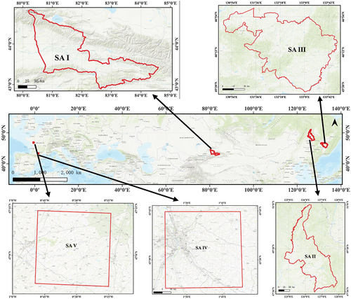
This study encompasses five distinct study areas. The first study area is located in the northwestern part of China and features primary crops such as maize, rice, wheat, and soybeans. The second and third study areas are located in the northeastern region of China, with soybeans, rice, and maize as the primary crops. The fourth and fifth study areas are located in the south and west-central part of France, where the main crops are wheat and maize. In the context of transfer learning experiments, Study Area I (SA I) and Study Area IV (SA IV) serve as the source domain, while Study Area II (SA II), Study Area III (SA III), and Study Area V (SA V) are designated as target domains. The geographical locations of the study area are illustrated in Figure 1.

Figure 1. Geographic location of the five study areas. Study area I is located in northwestern China, study area II and study area III are located in northeastern China, study area IV is located in southern France, and study area V is located in west-central France. The bottom image is World_Topo_Map. The red boundary is the geographic boundary of the study area.

2.2. Data

2.2.1. Satellite imagery

We used remote sensing images from the GaoFen-1 satellite with a temporal resolution of 4 days and a spatial resolution of 16 m for SA I, SA II, and SA III. The remote sensing images contain four bands: Blue, Green, Red, and NIR. The remote sensing images from March 1 to November 1 were selected for the time-series analysis according to the crop cultivation rules and the climatic conditions of the two regions. Effective acquisition dates for remote sensing imagery within each study area can be seen in Figure S1a. Remote sensing images with more than 10% cloudiness between March 1 and November 1 are removed, and remote sensing images with less than 10% cloudiness are subjected to a de-cloud operation, which can lead to inconsistencies in the length of the time series within the study area. To mitigate the impact of irregular time series, we performed resampling at 10-day intervals (Figure S1b), with missing values replaced by the average of the nearest valid values before and after the Day of the Year (DOY).

In SA Ⅳ and SA Ⅴ, we used Sentinel 2 remote sensing imagery with a spatial resolution of 10 m and a temporal resolution of 5 days. Remote sensing imagery from January 1 to December 31 was used for the time-series analysis (Figure S1a). The cloudiness screening in Sentinel 2 is consistent with GaoFen-1.

2.2.2. Ground truth data

2.2.2.1. Sample collection

Field surveys were conducted in 2017 and 2018 to collect labeled samples for SA I, SA II, and SA III. Sampling teams visited each region in July, with specific dates set for SA I in 2017 (July 14–21) and both SA II and SA III in 2017 (July 14–21) and 2018 (July 10–16). Each team consisted of three members: a leader to guide the sampling route and two assistants to document observations on either side. Sampling routes were strategically planned, leveraging knowledge of crop distribution and site accessibility. Data collection utilized the OvitalMap GIS application on mobile phones for recording crop boundaries, types, and growth conditions, excluding areas under 256 m² to maintain pixel integrity. Considering the time constraints of fieldwork may overlook some sample details, necessitating post-survey processing to refine and correct the collected data to result in detailed vector samples (polygons). These polygons were then mapped onto remote sensing images to construct a comprehensive crop time series. Figure 2 provides a detailed visual representation of the entire process, from the collection of field samples to the development of time series.

Figure 2. Pixel-level crop time series development process. (a) OvitalMap GIS application sampling interface, blue indicates sampling patches, black shows sampling information, and red indicates sampling routes. (b) QGIS software sample post-processing interface, red boxes indicate vector samples. (c) Overlaying vector samples with multi-temporal remote sensing images. (d) Pixel-level crop time series with DOY. Step 1 represents sample post-processing, step 2 represents vector sample overlay, and step 3 represents crop time series extraction.

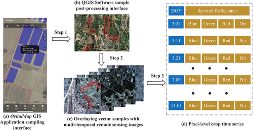
The vector samples for SA IV and SA V were sourced from (Nyborg et al. 2022), recording information including crop type and plot polygon. Since this data has been post-processed, the crop time series can be obtained directly by Figure 2c,d.

2.2.2.2. Sample dataset

In this study, the labeled samples in SA I and SA IV are sufficient while in SA II, SA III, and SA V are limited. SA II and SA III have labeled samples in 2017 and 2018, in the other study areas only 2017 exists. In SA I, SA II, and SA III, the common crops are maize, rice, and soybean, and the common crops are wheat, beans, maize, and barley in SA IV and SA V. The number of valid pixels for each category is shown in Table 1.

Table 1. Total number of valid pixels and crop types in each study area.

Year	2017					2018
	SA I	SA II	SA III	SA IV	SA V	SA II	SA III
Rice	30,771	39	197	–	–	139	70
Wheat	–	–	–	120,154	563	–	–
Maize	171,126	440	515	67,010	268	896	722
Soybeans	9,457	1,207	571	–	–	896	223
Beans	–	–	–	36,159	404	–	–
Barely	–	–	–	44,344	328	–	–
Other	25,584	364	197	–	–	277	84
Total	236,938	2,050	1,480	267,667	1,563	2208	1,099

Stage 2. Calculating IRDCTS between individual labeled samples.

3. Methods

In this study, we proposed two solutions to address the problems of crop classification in regions with limited labeled samples, focusing on both the classification model and the transfer strategy. The first solution aims to enhance the classification capabilities of the local crop classification model, maximizing the utilization of limited labeled samples. The second solution focuses on improving the adaptability of the source domain crop classification model to the target domain, harnessing the full potential of the source domain classification model. In the following two sections, we will introduce the designed classification model and the transfer strategy in detail.

3.1. Variable-dimension position symmetric net

The Variable-dimension Position Symmetric Net (VPSNet) receives a pixel-level time series including spectral reflectance and acquisition timing during the crop growing season. The model employs blocks with variably dimensional hidden layers to extract various forms of semantic features and a symmetric network structure to ensure the original time-series length is aligned with the feature dimensions of the model output. The specific network architecture is illustrated in Figure 3. The VPSNet model contains three components: the input module, the VPSNet module, and the output module.

Figure 3. The detailed structure of VPSNet-B. There are three types of VPSNet: VPSNet-b, VPSNet-s, and VPSNet-L. VPSNet-B denotes the base model with 11 blocks and the dimension of the intermediate block hidden layer is 64 d. VPSNet-S denotes the small model with 9 blocks and the dimension of the intermediate block hidden layer is 32 d. VPSNet-L denotes the large model with 13 blocks and the dimension of the intermediate block hidden layer is 128 d.

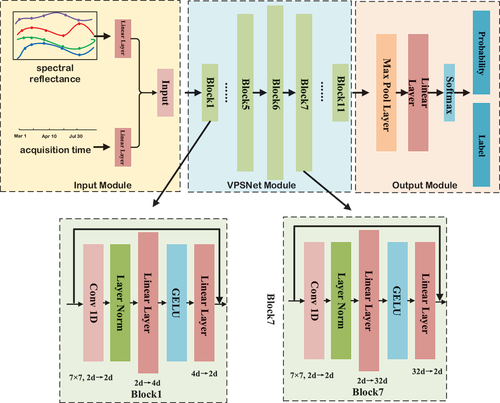
Input module: The spectral reflectance $\left[\mathit{s}{e}_1,\mathit{s}{e}_2,\dots ,\mathit{s}{e}_T\right]$ of each pixel is encoded as a d-dimensional spectra feature vector$\mathit{s}{f}_i$by equation (1)(1) $\mathit{s}{f}_i=\mathit{f}\left(\mathit{s}{e}_i\right)$(1) and T denotes the length of the time series, $\mathit{i}\in [0,\mathit{\hspace{0.17em}}\mathit{T}]$. The acquisition time of spectral reflectance$\left[\mathit{do}{y}_1,\mathit{do}{y}_2,\dots ,\mathit{do}{y}_T\right]$is encoded as a d-dimensional temporal feature vector$\mathit{t}{f}_i$by equation (2)(2) $\mathit{t}{f}_i\left(\mathit{p}\right)=\left\{\begin{array}{c}sin\left(\mathit{do}{y}_i/{1000}^{2\mathit{k}/d}\right)\mathit{\hspace{0.17em}}\mathit{if}\mathit{\hspace{0.17em}}\mathit{p}=2\mathit{k}\\ cos\left(\mathit{do}{y}_i/{1000}^{2\mathit{k}/d}\right)\mathit{\hspace{0.17em}}\mathit{if}\mathit{\hspace{0.17em}}\mathit{p}=2\mathit{k}+1\end{array}\right.$(2) . The spectral and temporal features concat into $x_i$ by equation (3)(3) $x_i=\mathrm{Concat}\left(\mathit{t}{f}_i,\mathit{s}{f}_i\right)$(3) as the input to the model.

(1) $\mathit{s}{f}_i=\mathit{f}\left(\mathit{s}{e}_i\right)$(1)

(2) $\mathit{t}{f}_i\left(\mathit{p}\right)=\left\{\begin{array}{c}sin\left(\mathit{do}{y}_i/{1000}^{2\mathit{k}/d}\right)\mathit{\hspace{0.17em}}\mathit{if}\mathit{\hspace{0.17em}}\mathit{p}=2\mathit{k}\\ cos\left(\mathit{do}{y}_i/{1000}^{2\mathit{k}/d}\right)\mathit{\hspace{0.17em}}\mathit{if}\mathit{\hspace{0.17em}}\mathit{p}=2\mathit{k}+1\end{array}\right.$(2)

(3) $x_i=\mathrm{Concat}\left(\mathit{t}{f}_i,\mathit{s}{f}_i\right)$(3)

where$\mathit{k}\in [0,\mathit{\hspace{0.17em}}\mathit{d}]$, d is the dimensionality of the feature vector.

VPSNet module: In VPSNet, each block with a different hidden layer depth extracts features from the input vector at different levels. While the intermediate layer depth of each block varies with the number of blocks, the depth of the input layer and the output layer remains the same to ensure that the input to each block remains consistent with the initial input. Additionally, we employed a residual structure (He et al. 2016) in each block to prevent the gradient from vanishing during the training process. The relationship between the hidden layer vector h, input vector input, and output vector output for each block can be represented as:

(4) $\mathit{inpu}{t}^l=\mathit{outpu}{t}^{\mathit{l}-1}+\mathit{inpu}{t}^{\mathit{l}-1}$(4)

(5) $\begin{array}{rl}& h_{l_1}^{\mathit{l}}=\mathit{LayerNorm}\left(w_{l_1}^{\mathit{l}}\ast \left(\mathrm{inpu}{\mathrm{t}}^l\right)+b_{l_1}^{\mathit{l}}\right)\\ & \mathit{\hspace{0.17em}}{h}_{l_2}^{\mathit{l}}=\mathit{act}\left(w_{l_2}^{\mathit{l}}\ast \left(h_{l_1}^{\mathit{l}}\right)+b_{l_2}^{\mathit{l}}\right)\\ & \mathit{\hspace{0.17em}}\mathit{outpu}{t}^l=w_{l_3}^{\mathit{l}}\ast \left(h_{l_2}^{\mathit{l}}\right)+b_{l_3}^{\mathit{l}}\end{array}$(5)

where l denotes the lth block, $l_i$denotes the ith hidden layer in the lth block, w and b denote the weight matrix that can be learned, and * denotes the convolution operation. act is $\mathit{GELU}\left(\mathit{x}\right)=0.5\mathit{x}(1+tanh(\sqrt{2/\mathit{\pi }}(\mathit{x}+0.044715x^3))$. GELU can significantly reduce the problem of gradient disappearance during training and can accelerate the convergence of the model. LayerNorm is used for the first layer of convolution operation due to it is more effective than BatchNorm for sequence processing (Liu et al. 2022). The first hidden layer is composed of one-dimensional convolution with a kernel size is 7. The last two hidden layers consist of Linear Layers to extract features in multiple dimensions. Compared to traditional CNN network structures, VPSNet employs fewer activation layers to reduce the risk of overfitting. Previous network structures used fixed combinations of convolution followed by activation functions, while one activation function is only used in a single block of VPSNet to reduce the interference of nonlinear operations in feature propagation. The use of the reverse bottleneck structure allows VPSNet to reduce the number of parameters while maintaining competitive performance and improving the overall efficiency of the model.

Output module: This module consists of a Global Maximum Pooling Layer and a Linear Layer. The Linear Layer output vector is computed using Softmax to obtain the classification labels and classification probabilities.

Compared to the prior study, the proposed deep learning model introduces several key distinctions: (1) Our model uniquely integrates spectral reflectance and the acquisition timing of this reflectance as inputs to address a gap in existing models that neglect the temporal aspect, leading to suboptimal feature extraction in regions with limited labeled (H. Wang et al. 2022; Zhong, Hu, and Zhou 2019). (2) To enhance the analysis of crop time-series data, we adopted a symmetric network structure to optimize the use of crop time-series information by ensuring that the input and output vectors are dimensionally congruent. (3) The introduction of blocks with variable dimensions for feature extraction allows our model to adeptly handle the extraction of complex semantic features, essential in contexts with limited labeled samples. This architectural design promotes feature diversity and aligns with the necessity for input-output dimension parity.

3.2. Design of IRDCTS

Utilizing models trained in regions with sufficient labeled samples for predictions in regions with limited label samples can be promising (Xu et al. 2020). However, discrepancies such as regional climate differences and cultivation practices can impede the direct applicability of models from the source domain to the target domain. The existence of limited labeled samples in the target region presents an opportunity to mitigate these challenges. In this study, we propose the IRDCTS to improve the source domain models’ adaptability to the target domain, detailed as follows:

Stage 1. Representative labeled sample selection.

To accurately compute the IRDCTS, we developed a method for the extraction of representative labeled samples from both the source and target domains. This method employs sampling route segmentation to divide into 1.5-kilometer segments. In each segment, one labeled sample is selected every 1.5 kilometers specifically for IRDCTS computation and initiation points of sampling vary across different crops. In instances where a segment lacks available samples, the process advances to the subsequent segmentation point. The quantity of labeled samples employed in the IRDCTS calculation is documented in Table 2.

Table 2. The number of labeled samples used to calculate IRDCTS.

Year	2017					2018
	SA I	SA II	SA III	SA IV	SA V	SA II	SA III
Rice	35	5	18	–	–	11	27
Wheat	–	–	–	35	28	–	–
Maize	30	26	27	24	36	29	31
Soybeans	22	35	24	–	–	34	31
Beans	–	–	–	31	27
Barely	–	–	–	29	19	–	–
Total	87	66	69	119	110	74	89

Stage 2. Calculating IRDCTS between individual labeled samples.

The inspiration for the IRDCTS is derived from image-denoising techniques (Tian et al. 2020). This technique shows that the noise between the noisy image and the noise-free image is spread over each pixel. Analogously, in the context of crop time-series analysis, the source domain’s time series can be regarded as “pure,” whereas the target domain’s time series is “noisy,” with the noise manifesting specifically in the acquisition time of spectral reflectance in time series. The multiplicative noise calculation method is employed to compute IRDCTS, as delineated in Equation (6)(6) $\mathit{y}(\mathit{i})=\mathit{x}(\mathit{i})+\mathit{g}(\mathit{i})\cdot \mathit{x}(\mathit{i})$(6)

(6) $\mathit{y}(\mathit{i})=\mathit{x}(\mathit{i})+\mathit{g}(\mathit{i})\cdot \mathit{x}(\mathit{i})$(6)

where y(i) and x(i) denote the crop time series of the target and source domains, respectively, and g(i) denotes IRDCTS between individual labeled samples.

Stage 3. Calculating IRDCTS.

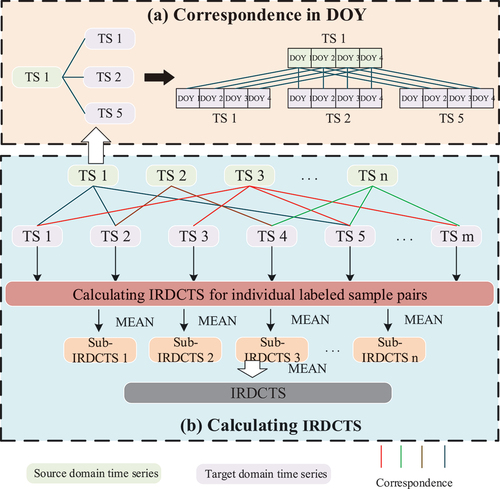
The primary challenge in computing the IRDCTS centers on efficiently matching labeled samples between the source and target domains. Direct one-to-one cross-matching is computationally intensive. To address this, we implemented a random matching strategy, illustrated in Figure 4b. This strategy begins with using source domain samples as bases for matching, and target domain samples as candidates for match-pairing. We then imposed a limit, denoted as L, on the number of possible matches per source domain sample, allowing for the random selection of 1 to L samples from the target domain for matching. The IRDCTS is represented by the mean of the sub-IRDCTS calculated for these sample pairs.

Figure 4. Correspondence between crop time series and IRDCTS calculation process. (a) Correspondence in DOY. (b) Calculating IRDCTS. (a) shows the correspondence rules for time series between individual pixel pairs.(b) shows the process of calculating the sub-irdcts for an individual pixel pair and the process of calculating the IRDCTS between the source and target domains.

Calculate IRDCTS

1 Input: source domain labeled sample set LS_s=[ts₁, ts₂, … , ts_n], target domain labeled sample set LS_t=[ts₁, ts₂, … , ts_m], where ts_i =[ts_i1,ts_i2, … ,ts_iT] denotes the ith time series of length T, m and n denote the number of labeled sample

2 Select k representative labeled samples LS_sr in the source domain and z representative labeled samples LS_tr in the target domain

3 for j = 1 to k do

4 Randomly select L target domain labeling samples (L≤z)

5 for jj = 1 to L do

5 Calculating the IRDCTS between LS_sr_j and LS_tr_jj by $\mathit{IRDCT}{S}_{\mathit{jj}}=\frac{\mathit{LS}\_\mathit{t}{\mathit{r}}_{\mathit{jj}}-\mathit{LS}\_\mathit{t}{r}_j}{\mathit{LS}\_\mathit{t}{r}_j}$

6 Calculate IRDCTS for L sample pairs $\mathit{IRDCT}{S}_j=\mathit{Mean}(\mathit{IRDCT}{S}_1,\dots ,\mathit{IRDCT}{S}_L)$

7 Calculate IRDCTS for k sample pairs $\mathit{IRDCT}\mathit{S}=\mathit{Mean}(\mathit{IRDCT}{S}_1,\dots ,\mathit{IRDCT}{S}_k)$

8 Output: IRDCTS

4. Experimental design

4.1. Different forms of network structures

To assess the efficacy of the proposed VPSNet, we undertook a detailed comparison involving five distinct network structures as depicted in Figure 5. To guarantee an equitable evaluation, each network configuration maintained a consistent number of blocks. Below is a succinct overview of the five network structures evaluated:

Figure 5. The different sections between the five different network structures and VPSNet. ID indicates that the dimensionality of the hidden layer within the block remains invariant. IONR indicates that the dimensionality of the hidden layer within the block is non-asymmetric.NoPE indicates that only the spectral reflectance serves as the input for the classification model.Us indicates that the classification model presents an upsampling form. DS indicates that the classification model exhibits a downsampling form.

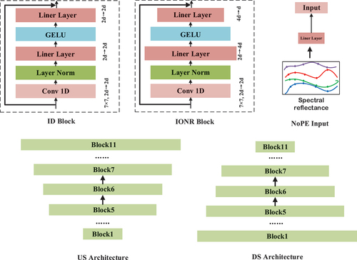
Invariant Dimensional (ID): This structure characterizes uniform hidden layer dimensions, with inputs and outputs for each block maintaining identical dimensions, resulting in a symmetrical structure.

Up-Sampling (US): This structure characterizes increasing hidden layer dimensions, with inputs and outputs for each block maintaining identical dimensions, resulting in an asymmetrical structure.

Down-Sampling (DS): This structure characterizes decrement hidden layer dimensions, with inputs and outputs for each block maintaining identical dimensions, resulting in an asymmetrical structure.

Input-Output Non-Reciprocal (IONR): This structure characterizes various hidden layer dimensions, with inputs and outputs for each block maintaining different dimensions, resulting in a symmetrical structure.

No Position Encoding (NoPE): This structure is consistent with the hidden layer variations of VPSNet but without positional encoding.

4.2. Different transfer strategies in transfer learning

Three different IRDCTS applications were set up to evaluate the effectiveness of ISDCTS. In scenarios where IRDCTS is not utilized during model transfer termed Transfer Learning without Transfer Strategy (TL1). Conversely, employing IRDCTS in the transfer process is designated as Transfer Learning with a Transfer Strategy. IRDCTS can be applied both in the source and target domains. Specifically, when applied in the source domain, IRDCTS adjusts the crop time series to align with the target domain’s time series via Equation (7)(7) $\hat{X}=\mathit{X}\left(1+\mathit{G}\right)$(7) , which is referred to as TL2. When implemented in the target domain, IRDCTS adjusts the crop time series to align with the target domain’s time series via Equation (8)(8) $\hat{X}=\frac{X}{\left(1+\mathit{G}\right)}$(8) , which is referred to as TL3.

(7) $\hat{X}=\mathit{X}\left(1+\mathit{G}\right)$(7)

(8) $\hat{X}=\frac{X}{\left(1+\mathit{G}\right)}$(8)

where$\mathit{X}$denotes the unprocessed original crop time series, $\hat{X}$denotes the processed crop time series using IRDCTS, and G represents IRDCTS.

4.3. Experimental setup and accuracy assessment

The block number of VPSNet was set to (9, 11, 13), with an initial hidden layer dimension of 256. The training process involved SA I and SA IV with epoch = 100, SA II, SAIII, and SA V with epoch = 1000, a batch size of 256, a learning rate of 1e-5, and a dropout rate of 0.1. The optimizer is Adam, and the loss function is cross-entropy.

The entire experiment was run on a Windows platform configured with an i7–11700 K @ 3.60 GHz, 32 G RAM, and NVIDIA GeForce RTX 3080 GPU (10 GB RAM), and all programs were written using the Python language.

In this study, several evaluation metrics were used to evaluate the proposed transfer strategy and classification model. Overall Accuracy (OA) was used to evaluate the classification accuracy of the classification model and the overall performance of the transfer strategy. Recall, Precision, F1 scores, and F2 scores were used to assess the classification ability of the classification methods for different crops.

(9) $\mathit{OA}=\frac{{\mathit{n}}^{\mathit{corr}}}{n^{\mathit{all}}}$(9)

(10) $\mathrm{Recal}{\mathrm{l}}_c=\frac{n_c^{c\mathrm{orr}}}{n_c^k}$(10)

(11) $\mathrm{Precisio}{\mathrm{n}}_c=\frac{n_c^{c\mathrm{orr}}}{n_c^l}$(11)

(12) $\mathit{F}{1}_c=2\frac{\mathrm{Recal}{\mathrm{l}}_c\ast \mathit{precisio}{n}_c}{\mathit{precisio}{n}_c+\mathrm{Recal}{\mathrm{l}}_c}$(12)

(13) $\mathit{F}{2}_c=5\frac{\mathrm{Recal}{\mathrm{l}}_c\ast \mathit{precisio}{n}_c}{4\mathit{precisio}{n}_c+\mathrm{Recal}{\mathrm{l}}_c}$(13)

where n^corr represents the number of labeled samples correctly classified, n^all denotes the number of samples used for validation. $n_c^k$ denotes the number of true samples in category c, and $n_c^l$ denotes the number predicted to be in category c.

4.4. Experimental training and validation

4.4.1. Local training and validation

VPSNet underwent evaluation in study areas SA II (2017, 2018), SA III (2017, 2018), and SA V (2017) in localized testing. The distribution of labeled samples across these regions (calculated by subtracting the number of samples in Table 2 from those in Table 1) was allocated into training, validation, and testing sets following a 4:2:4 ratio. In localized testing, VPSNet was compared against six network architectures alongside six competitive crop classification methodologies. The six methods were RF, DeepCropMapping (DCM) (Xu et al. 2020), SITS-BERT (Yuan and Lin 2021), Conformer (Gulati et al. 2020), Performer (Choromanski et al. 2021), and Cropformer (H. Wang et al. 2023).

4.4.2. Transfer learning training and validation

Evaluation of IRDCTS in transfer learning in SAI_SAII, SAI_SAIII, and SAIV_SAV. Specifically, in SA I and SA IV, the distribution of the dataset into training, validation, and testing sets adhered to a 6:2:2 ratio. It should be noted that training and validation sets were derived exclusively from SA I and SA IV, whereas testing sets were sourced from SA II, SA III, and SA V. The effectiveness of IRDCTS was assessed using four distinct classification methods, namely RF, SITS-BERT (Yuan and Lin 2021), Cropformer (H. Wang et al. 2023), and VPSNet, to determine its viability across various models.

5. Results

5.1. Evaluation of VPSNet

Table 3 reports the accuracy of VPSNet across three different scales and six competitive classification models. Compared to DeepCropMapping (DCM) at the same scales, VPSNet-S showed an accuracy advantage in three out of five classification scenarios. VPSNet-B performed impressively, with a cumulative accuracy exceeding that of SITS-BERT (20.54%), Cropformer (15.61%), Conformer (4.07%), and Performer (8.54%) in the five classification scenarios indicating VPSNet could extract more discriminative features with fewer parameters. VPSNet-L outperformed all models in the five classification scenarios, achieving a cumulative accuracy surpassing the top-performing methods, RF (18.08%), Performer (17.74%), and Conformer (13.27%), highlighting the superiority in fully leveraging the information from limited labeled samples of VPSNet.

Table 3. OA of different classification models in five classification scenarios (%).

Methods	2017_SA II	2017_SA III	2018_SA II	2018_SAIII	2017_SA V	Parameter count
RF	78.35	63.45	80.49	71.91	83.38	1k <
SITS-BERT	76.31	62.36	78.13	69.42	80.06	24 M
Cropformer	80.14	61.56	78.54	67.16	83.81	28 M
Conformer	80.49	65.19	77.45	76.17	83.45	31 M
DCM	77.32	64.01	77.70	69.23	82.68	5 M
Performer	77.37	60.82	80.73	75.32	84.04	30 M
VPSNet-S	81.05	62.87	79.51	71.06	82.40	7.6 M
VPSNet-B	81.27	66.49	82.44	73.19	83.43	16 M
VPSNet-L	83.21	68.42	81.71	78.21	84.47	31 M

Bold indicates best.

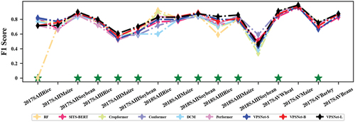
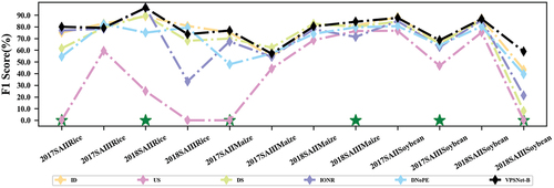
Figure 6 shows the F1 scores of different models in each classification scenario. VPSNet achieved the best performance in 11 out of the 16 crop types. The advantage of VPSNet over the other five models was more significant for very limited labeled samples, such as 2017 SAII Rice, further demonstrating the superiority of the proposed approach. Another classification accuracy for three experiments could be found in Figure S2. Specifically, VPSNet achieved the highest recall in 8 out of 16 crop types, as well as the highest precision in 8 out of 16 crop types, as well as the highest F2 scores in 11 out of 16 crop types, and was also generally in a suboptimal position or at the top of the list in non-optimal scenarios (e.g. 2017SAIIRice and 2018SAIIIRice).

Figure 6. F1-score per crop type (%) of different classification models in different classification scenarios. Green * indicates that VPSNet obtains the highest accuracy in this scenario.

5.2. Evaluation of IRDCTS in transfer learning

Table 4 reports the classification accuracy using different transfer strategies in regions with limited labeled samples. In the five classification scenarios, all four classification models using TL1 were ineffective in the target domain, with classification accuracy exceeding 60% only in 2018_SAIII, indicating cross-region model transfer may not be effective without considering domain discrepancies. Comparing TL3 to TL1, the minimum improvement in OA exceeded 24%, with the maximum improvement exceeding 70%, while compared to TL 2, the minimum improvement in OA exceeded 9%, with the maximum improvement exceeding 45%. The results showed that IRDCTS significantly improved the classification performance of cross-region model transfer, indicating that transfer learning could address the crop classification problem in regions with limited labeled samples, provided that the model trained in the source domain could adapt to the target domain’s classification scenarios. The results of SA II and SA III in 2018 showed that IRDCTS could accommodate transfer scenarios across years and regions, implying that the choice of source domains is not limited by year, which provided better options for large-scale model transfer.

Table 4. OA of different transfer learning strategies using different classification models (%).

Methods	Transfer strategy	2017_SA II	2017_SA III	2018_SA II	2018_SA III	2017_SA V
RF	TL 1	7.40	31.13	26.97	68.81	26.32
	TL 2	53.85	46.36	61.58	42.66	52.35
	TL 3	68.34	81.79	81.07	92.66	72.36
SITS-BERT	TL 1	6.80	29.80	19.77	62.11	48.36
	TL 2	64.50	48.68	68.08	43.12	60.36
	TL 3	83.79	83.71	77.01	91.58	78.05
CT	TL 1	6.73	28.48	23.45	64.22	40.23
	TL 2	71.01	51.66	73.73	62.39	56.33
	TL 3	82.54	83.74	81.36	89.91	76.35
VPSNet-B	TL 1	7.99	36.75	26.27	51.38	46.03
	TL 2	63.91	49.34	49.34	40.83	58.58
	TL 3	82.66	90.07	82.49	90.83	78.60

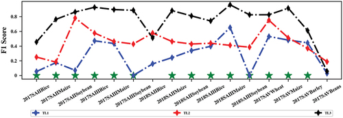
Figure 7 provides the F1 scores for different transfer strategies using VPSNet-B in each classification scenario. Almost all scenarios reached significant improvement in F1 scores by using IRDCTS. In some scenarios such as 2017_SAIII Maize, 2018_SAIII Maize, and 2018_SAIII Rice, the use of IRDCTS resulted in lower or close performance for TL 2 compared to TL 1 possibly due to more noise adulteration of the samples generated in the source domain. Another classification accuracy for three experiments can be found in Figure S3. Specifically, VPSNet achieved the highest recall in 11 out of 16 crop types, the highest precision in 14 out of 16 crop types, and the highest F2 score in 13 out of 16 crop types.

Figure 7. F1-score per crop type (%) of different transfer learning strategies using VPSNet-B. Green * indicates that TL3 obtains the highest accuracy in this scenario.

5.3. Comparing two proposed solutions

In this set of experiments, we compared two proposed solutions for crop classification in regions with limited labeled samples. This comparison was conducted on classification accuracy and mapping results, utilizing (You et al. 2021) as the reference mapping and accuracy (Figure S5). For the mapping, two areas measuring 10 km × 10 km each in SA II and SA III were selected for detailed crop mapping, focusing on rice, maize, and soybeans. In Solution 2, the mapping process for each area involved three iterations for the specific crops (rice, maize, and soybeans), and only the mapping results of the target crops were preserved during iteration. The pixels with the highest confidence among the three results were retained as the final mapping result.

Table 5 reports the classification results of the two solutions in five classification scenarios. Compared Solution 2 to Solution 1, notably achieving substantial overall accuracy (OA) improvements in 2017 SA III and 2018 SA III by 21.65% and 12.62%, respectively. Although VPSNet could adapt to classification scenarios with limited labeled samples, its adaptability was still insufficient compared to models trained with sufficient labeled samples in the source domain. Solution 1 obtained the best F1 score in six classification scenarios while Solution 2 performed the best F1 score in eight classification scenarios in Figure 8. Other metrics for Solutions 1 and 2 are shown in Figure S4. Overall, Solution 2 exhibits a more pronounced advantage in terms of accuracy in regions with limited labeled samples.

Figure 8. F1-score per crop type (%) of different solutions.

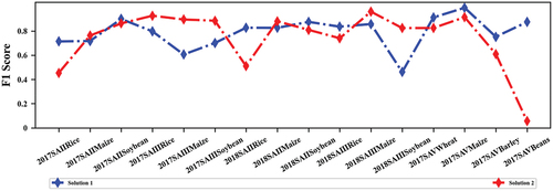
Table 5. OA of different solutions in five classification scenarios (%).

Classification Scenarios	2017_SA II	2017_SA III	2018_SA II	2018_SA III	2017_SA V
Solutions 1	83.21	68.42	81.71	78.21	84.47
Solutions 2	82.66	90.07	82.49	90.83	78.60

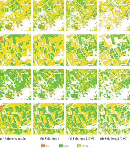
Figure 9 shows the mapping results of different solutions compared to the reference mapping results. Solution 1 mapping results had the highest similarity with the reference mapping results, Solution 2 with threshold 0.95 was second, and Solution 2 with threshold 0.99 was the worst. Compared to the reference mapping, the majority of pixels in the mapping results of both solutions were correctly classified, indicating that our solutions effectively addressed crop classification issues in regions with limited labeled samples. Although there were some inconsistencies between our results and the reference mapping, the reference mapping was based on sufficient labeled samples and had undergone effective post-processing. SA II and SA III implemented crop rotation between soybeans and maize, and our mapping results for 2017–2018 are consistent with this. A large number of pixels with classification probabilities less than 99% were excluded in Solution 2, resulting in visually worse mapping results for Solution 2 than for Solution 1 (Figure 9(c)). The mapping results for Solution 2 were improved when the screening threshold was lowered to 95%. In conclusion, both solutions effectively addressed the crop classification problem in regions with limited labeled samples. Solution 1 achieved lower accuracy compared to Solution 2, but its mapping results were generally superior to Solution 2. So, we recommend using Solution 1 when labeled samples are moderately available, while Solution 2 could be employed in scenarios with extremely limited. Note that the use of Solution 2 presupposes the existence of sufficient labeled source domains, otherwise Solution 1 is still the best choice.

Figure 9. Comparison of mapping results of different solutions in four classification scenarios. The first and third rows represent the mapping results for SA III, while the second and fourth rows represent the mapping results for SA II.

6. Discussions

6.1. The advantages of the VPSNet structure

In exploring the efficacy of various network structures in regions with limited labeled samples, six distinct structures were evaluated, as detailed in Section 4.1. TheVPSNet showed performance improvement over five structures in four classification scenarios (Table 6). The US structure exhibited the lowest performance, suggesting that the increase in asymmetric hidden layer dimensions introduces unnecessary redundancy. The IONR structure was the second least effective, primarily due to its disruption of sequence information caused by mismatched input and output dimensions. The ID structure, despite utilizing fewer parameters, achieved near-optimal results. Similarly, the DS structure demonstrated commendable performance, reinforcing the significance of preserving dimension consistency between input and output in crop classification. The NoPE structure yielded a close but unstable performance as compared to VPSNet, possibly due to a lack of understanding of temporal information.

Table 6. OA of different network structures in four classification scenarios (%).

Network structures	2017_SA II	2017_SA III	2018_SA II	2018_SA III	Parameter count
ID	80.27	65.50	80.73	72.34	98k
US	64.23	47.66	66.59	62.13	24 M
DS	76.89	66.67	80.73	68.94	24 M
IONR	76.89	61.99	77.80	57.87	17 M
NoPE	71.53	65.20	73.66	71.49	16 M
VPSNet-B	81.27	66.49	82.44	73.19	16 M

Figure 10 illustrates the F1 scores for various network structures across different crop types over 2 years. VPSNet-B outperformed other network structures in half among the 12 evaluated scenarios, demonstrating its robustness and structural advantages. For certain scenarios, VPSNet-B was to also be in sub-optimal accuracy such as 2017_SA II soybeans and 2018_SA II soybeans. Other network structures showed unstable performance. For example, the US structure recorded 0% accuracy for rice and maize in 2017 SA II yet showed remarkable performance for soybeans. In some scenarios, VPSNet underperformed DS and ID structures such as 2017_SA III maize and 2018_SA III rice, which may be due to the introduction of redundant information in the up-sampling.

Figure 10. F1-score per crop type (%) of different network structures. Green * indicates that VPSNet-B obtains the highest accuracy in this scenario.

6.2. Evaluation of model inputs for solutions 1 and 2

To demonstrate the effectiveness of the proposed solution with other bands and vegetation indices as inputs, we conducted comparative experiments in SA IV and V. In this set of experiments, Sentinel 2 imagery served as the primary data source, with model inputs segmented into four distinct categories for analysis. The first category of input included the blue, green, red, and near-red spectral bands. Input 2 expanded upon input1 by adding short-wave infrared 1 (SWIR1) and short-wave infrared 2 (SWIR2) bands. Input 3 adds vegetation indices including the Normalized Difference Vegetation Index (NDVI), Enhanced Vegetation Index (EVI), Ratio Vegetation Index (RVI), and Green Normalized Difference Vegetation Index (GNDVI) to input1. Input 4 then adds the vegetation index to input 2.

Table 7 reports the accuracy of different classification models using different inputs in the SA V. VPSNet yielded a higher OA than other classification models with different inputs indicating VPSNet can adapt to different spectral datasets. When the model inputs were enriched, the classification accuracy of almost all classification models was improved, implying that enriching the inputs to the models for regions with limited labeled samples was also feasible. The F1 scores for different crop types in SA V are shown in Figure 11 for comparison of different inputs.

Figure 11. F1 scores per crop type for classification models using different inputs. Green * indicates that VPSNet-L obtains the highest accuracy in this scenario.

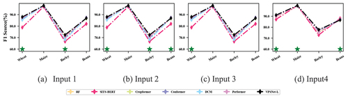
Table 7. OA of different classification models using different inputs (%).

Methods	RF	SITS-BERT	Cropformer	Conformer	DCM	Performer	VPSNet-L
Input 1	83.38	80.06	83.81	83.45	82.68	84.04	84.47
Input 2	83.46	82.37	83.17	83.93	83.43	83.62	83.99
Input 3	85.80	82.55	85.93	84.36	84.32	84.54	86.49
Input 4	85.93	85.08	86.23	86.78	86.22	86.16	87.11

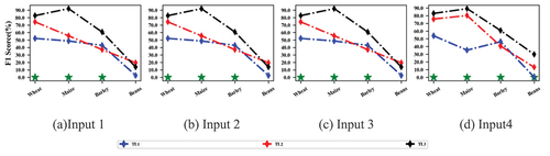
Table 8 reports the accuracy of different transfer strategies using different inputs in the SA V. TL3 consistently achieved notable accuracy improvements over both TL1 and TL2, validating the effectiveness of the IRDCTS with Sentinel 2. Comprised accuracy of different inputs can be observed that input 1 and input 2 yielded superior results compared to input 3 and input 4, especially when TL1 and TL2 were used. This might be because the inaccuracy of IRDCTS was further amplified by the addition of the vegetation index, as IRSCTS was only an approximation of the inter-domain discrepancies. The F1 scores for different crop types show TL3 using other bands and vegetation indices as input still outperformed the other two transfer strategies, further demonstrating the generality of IRDCTS (Figure 12).

Table 8. OA of different transfer strategies using different inputs (%).

Transfer strategy	TL1	TL2	TL3
Input 1	45.29	59.06	78.72
Input 2	49.88	67.88	80.22
Input 3	42.88	56.75	77.18
Input 4	42.11	52.03	77.54

Figure 12. F1 scores per crop type of different transfer strategies using different inputs (%). Green * indicates that TL3 obtains the highest accuracy in this scenario.

6.3. The necessity of IRDCTS

Contrasting the temporal profiles of crop time series between the source domain and the target domain allowed observation of variations in crop growth across different regions. The temporal profiles of SA II and SA III were very similar, while there were significant differences between SA I and SA II/III (Figure S6) suggesting that differences in temporal profiles between crops in geographically close and climatically similar regions were less likely to occur. Conversely, in regions with greater geographical separation and larger climate differences, there were more noticeable differences in crop temporal profiles. This observation aligns with previous research findings (Lin et al. 2022; S. Wang, Azzari, and Lobell 2019). This was why we chose SA I as the source domain because selecting a source domain geographically close to the target domain will place both domains within the same ecological zone, which contradicted the setting of limited labeled samples. These differences in crop time series posed challenges to the transfer of classification models. Eliminating these differences was crucial for achieving successful cross-domain model transfer, making the use of IRDCTS essential in cross-domain model transfer.

6.4. Feasibility of crop mapping with solution 2

The precondition for crop mapping using Solution 2 (TL 3) is that the IRDCTS for different crops were distinct. We compared the temporal profiles of IRDCTS in four bands between 2017_SA I and 2018_SA II. The trends in IRDCTS across four bands varied for different crops (Figure S7), facilitating our use of Solution 2 for crop mapping. During the mapping process, it’s crucial to select the relevant IRDCTS based on the crops to map. Given that the same region may contain not only the target crop but also other crops, there is a risk of misclassifying non-target crops. In such cases, only pixels with classification probabilities exceeding 0.95 and 0.99 are employed, and these high-confidence pixels are used for mapping. Additionally, these high-confidence labeled samples can serve as generated samples, presenting another solution to address crop classification in regions with limited labeled samples.

6.5. Interpretation of VPSNet performance

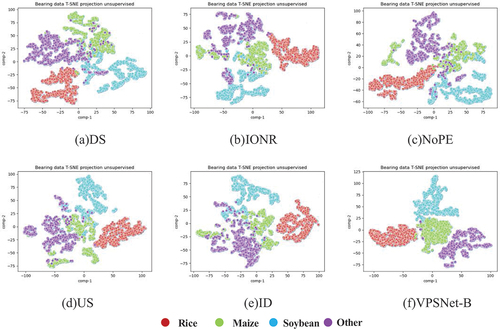
To further investigate the performance of VPSNet, we employed t-SNE to visualize the features learned from the six different structures. As shown in Figure 13, it is evident that for certain structures, the classification boundaries between some classes appear to be less distinct, such as the case of maize and soybeans in DS. In contrast, VPSNet exhibited clearer classification boundaries among the four classes. This observation suggested that the proposed network structure was effective in extracting features with higher discriminative power.

Figure 13. t-SNE visualization of the different network structures.

6.5.1. Limitations

This study has effectively addressed the issue of crop classification in regions with limited samples from both the perspectives of classification models and transfer strategies. However, there are still some limitations that need to be addressed in future research. In terms of classification models, this study utilized spectral reflectance and acquisition time of individual pixels’ time series as inputs for the classification model. However, the relationships between each pixel and its neighboring pixels were not considered. Incorporating such relationships could be a potential avenue for further improving the classification model’s performance in regions with limited labeled samples. Regarding transfer strategies, the method of segmenting routes was employed to obtain crop time series from both the source and target domains for calculating IRDCTS. While this approach had proven effective, its performance might be limited when sampling routes were not sufficiently diverse. In future work, exploring methods that consider the centroid of all labeled samples for IRDCTS calculation may reduce errors caused by insufficient diversity in the labeled sample. In addition, while this study was able to provide a solution for regions with limited labeled samples, it was limited in the help it provided for crop classification in sample-free regions. In future work, we will also explore crop categorization in sample-free regions from both deep learning and migration learning, possibly through domain adaptation techniques that tailor the model more closely to the target domain’s conditions (Y. Wang et al. 2022).

7. Conclusions

This study addresses the issue of crop classification in regions with limited labeled samples from two perspectives: deep learning and transfer learning. A novel deep learning model is proposed, which extracts different forms of semantic features by configuring different hidden layer depths. The results demonstrate that the proposed method exhibits advantages across various classification scenarios. Additionally, a new transfer strategy is introduced to enhance the adaptability of the source domain model in the target domain by reducing inter-domain discrepancies. The results show that, with the use of IRDCTS, the crop classification accuracy in the target domain can reach up to 90.83%. A comparison of the two solutions reveals that Solution 2 (classification strategy) outperforms Solution 1 (classification model) when labeled samples are extremely scarce, while Solution 1 performs better when labeled sample availability is strong. The temporal profiles of crop time series in different regions show that cross-domain model transfer is influenced by inter-domain differences, and IRDCTS can reduce these differences, thereby improving the model’s adaptability. Visualizations indicate that, compared to other network structures, VPSNet can learn clearer classification boundaries between crops.

Disclosure statement

No potential conflict of interest was reported by the author(s).

Data availability statement

The labeled sample data that support the findings of this study are available on request from the corresponding author upon reasonable request. GF 1 images were developed by the China Resources Satellite Application Center (CRSAC) and are available from the Land Observing Satellite Data Service (LOSDS) website (https://data.cresda.cn/#/home.)

Supplementary material

Supplemental data for this article can be accessed online at https://doi.org/10.1080/15481603.2024.2387393.

Additional information

Funding

This work was supported in part by the National Natural Youth Science Foundation of China under Grant [42001352]; and in part by the National Key Research and Development Program of China under Grant [2022YFB3903500].

References

- Belgiu, M., W. Bijker, O. Csillik, and A. Stein. 2021. “Phenology-Based Sample Generation for Supervised Crop Type Classification.” International Journal of Applied Earth Observation and Geoinformation 95:102264. https://doi.org/10.1016/j.jag.2020.102264.
- Choromanski, K. M., V. Likhosherstov, D. Dohan, X. Song, A. Gane. 2021. “Rethinking Attention with Performers, International Conference on Learning Representations.”
- Franch, B., J. Cintas, I. Becker-Reshef, M. J. Sanchez-Torres, J. Roger, S. Skakun, J. A. Sobrino, et al. 2022. “Global Crop Calendars of Maize and Wheat in the Framework of the WorldCereal Project.” GIScience & Remote Sensing 59 (1): 885–20. https://doi.org/10.1080/15481603.2022.2079273.
- Franch, B., E. Vermote, I. Becker-Reshef, M. Claverie, J. Huang, J. Zhang, C. Justice, et al. 2015. “Improving the Timeliness of Winter Wheat Production Forecast in the United States of America, Ukraine and China Using MODIS Data and NCAR Growing Degree Day Information.” Remote Sensing of Environment 161:131–148. https://doi.org/10.1016/j.rse.2015.02.014.
- Gallego, J., M. Craig, J. Michaelsen, B. Bossyns, and S. Fritz. 2008. Best Practices for Crop Area Estimation with Remote Sensing. Ispra: Joint Research Center.
- Gulati, A., J. Qin, C.-C. Chiu, N. Parmar, Y. Zhang. 2020. “Conformer: Convolution-Augmented Transformer for Speech Recognition.” https://doi.org/10.48550/arXiv.2005.08100.
- Hao, P. Y., L. P. Di, C. Zhang, and L. Y. Guo. 2020. “Transfer Learning for Crop Classification with Cropland Data Layer Data (CDL) as Training Samples.” Science of the Total Environment 733:138869. https://doi.org/10.1016/j.scitotenv.2020.138869.
- Hao, P. Y., L. Wang, Y. L. Zhan, C. Y. Wang, Z. Niu, and M. Wu. 2016. “Crop Classification Using Crop Knowledge of the Previous-Year: Case Study in Southwest Kansas, USA.” European Journal of Remote Sensing 49 (1): 1061–1077. https://doi.org/10.5721/EuJRS20164954.
- He, K., X. Zhang, S. Ren, and J. Sun. 2016. “Deep Residual Learning for Image Recognition.” Proceedings of the IEEE conference on computer vision and pattern recognition, Las Vegas, USA, 770–778.
- Ji, S., C. Zhang, A. Xu, Y. Shi, and Y. Duan. 2018. “3D Convolutional Neural Networks for Crop Classification with Multi-Temporal Remote Sensing Images.” Remote Sensing 10 (1): 75. https://doi.org/10.3390/rs10010075.
- Johnson, D. M., and R. Mueller. 2021. “Pre- and Within-Season Crop Type Classification Trained with Archival Land Cover Information.” Remote Sensing of Environment 264:112576. https://doi.org/10.1016/j.rse.2021.112576.
- Konduri, V. S., J. Kumar, W. W. Hargrove, F. M. Hoffman, and A. R. Ganguly. 2020. “Mapping Crops within the Growing Season Across the United States.” Remote Sensing of Environment 251:112048. https://doi.org/10.1016/j.rse.2020.112048.
- Lin, C., L. Zhong, X.-P. Song, J. Dong, D. B. Lobell, and Z. Jin. 2022. “Early- and In-Season Crop Type Mapping without Current-Year Ground Truth: Generating Labels from Historical Information via a Topology-Based Approach.” Remote Sensing of Environment 274:112994. https://doi.org/10.1016/j.rse.2022.112994.
- Liu, Z., H. Mao, C.-Y. Wu, C. Feichtenhofer, T. Darrell. 2022. “A Convnet for the 2020s.” Proceedings of the IEEE/CVF Conference on Computer Vision and Pattern Recognition, New Orleans, USA, 11976–11986.
- Malambo, L., and C. D. Heatwole. 2020. “Automated Training Sample Definition for Seasonal Burned Area Mapping.” ISPRS J. Photogram. Remote Sens 160:107–123. https://doi.org/10.1016/j.isprsjprs.2019.11.026.
- Minh, D. H. T., D. Ienco, R. Gaetano, N. Lalande, E. Ndikumana, F. Osman, P. Maurel, et al. 2018. “Deep Recurrent Neural Networks for Winter Vegetation Quality Mapping via Multitemporal SAR Sentinel-1.” IEEE Geoscience & Remote Sensing Letters 15 (3): 464–468. https://doi.org/10.1109/LGRS.2018.2794581.
- Nyborg, J., C. Pelletier, S. Lefèvre, and I. Assent. 2022. “TimeMatch: Unsupervised Cross-Region Adaptation by Temporal Shift Estimation.” Isprs Journal of Photogrammetry & Remote Sensing 188:301–313. https://doi.org/10.1016/j.isprsjprs.2022.04.018.
- Pelletier, C., G. I. Webb, and F. Petitjean. 2019. “Temporal Convolutional Neural Network for the Classification of Satellite Image Time Series.” Remote Sensing 11 (5): 523. https://doi.org/10.3390/rs11050523.
- Skakun, S., B. Franch, E. Vermote, J.-C. Roger, I. Becker-Reshef, C. Justice, N. Kussul, et al. 2017. “Early Season Large-Area Winter Crop Mapping Using MODIS NDVI Data, Growing Degree Days Information and a Gaussian Mixture Model.” Remote Sensing of Environment 195:244–258. https://doi.org/10.1016/j.rse.2017.04.026.
- Skakun, S., N. Kussul, A. Y. Shelestov, M. Lavreniuk, and O. Kussul. 2016. “Efficiency Assessment of Multitemporal C-Band Radarsat-2 Intensity and Landsat-8 Surface Reflectance Satellite Imagery for Crop Classification in Ukraine.” IEEE Journal of Selected Topics in Applied Earth Observations & Remote Sensing 9 (8): 3712–3719. https://doi.org/10.1109/JSTARS.2015.2454297.
- Tian, C., L. Fei, W. Zheng, Y. Xu, W. Zuo, and C.-W. Lin. 2020. “Deep Learning on Image Denoising: An Overview.” Neural Networks 131:251–275. https://doi.org/10.1016/j.neunet.2020.07.025.
- Vaswani, A., N. Shazeer, N. Parmar, J. Uszkoreit, L. Jones. 2017. “Attention is All You Need.” Advances in Neural Information Processing Systems, Cambridge, MA, USA, 5998–6008.
- Venkatanaresh, M., and I. Kullayamma. 2022. “A New Approach for Crop Type Mapping in Satellite Images Using Hybrid Deep Capsule Auto Encoder.” Knowledge-Based Systems 256:109881. https://doi.org/10.1016/j.knosys.2022.109881.
- Wang, H., W. Chang, Y. Yao, D. Liu, Y. Zhao, S. Li, Z. Liu, et al. 2022. “CC-SSL: A Self-Supervised Learning Framework for Crop Classification with Few Labeled Samples.” IEEE Journal of Selected Topics in Applied Earth Observations & Remote Sensing 15:8704–8718. https://doi.org/10.1109/JSTARS.2022.3211994.
- Wang, H., W. Chang, Y. Yao, Z. Yao, Y. Zhao, S. Li, Z. Liu, et al. 2023. “Cropformer: A New Generalized Deep Learning Classification Approach for Multi-Scenario Crop Classification.” Frontiers in Plant Science 14. https://doi.org/10.3389/fpls.2023.1130659.
- Wang, L., Y. Bai, J. Wang, Z. Zhou, F. Qin, and J. Hu. 2023. “Histogram Matching-Based Semantic Segmentation Model for Crop Classification with Sentinel-2 Satellite Imagery.” GIScience & Remote Sensing 60 (1): 2281142. https://doi.org/10.1080/15481603.2023.2281142.
- Wang, S., G. Azzari, and D. B. Lobell. 2019. “Crop Type Mapping without Field-Level Labels: Random Forest Transfer and Unsupervised Clustering Techniques.” Remote Sensing of Environment 222:303–317. https://doi.org/10.1016/j.rse.2018.12.026.
- Wang, Y., L. Feng, W. Sun, Z. Zhang, H. Zhang, G. Yang, X. Meng, et al. 2022. “Exploring the Potential of Multi-Source Unsupervised Domain Adaptation in Crop Mapping Using Sentinel-2 Images.” GIScience & Remote Sensing 59 (1): 2247–2265. https://doi.org/10.1080/15481603.2022.2156123.
- Wang, Y., Z. Zhang, L. Feng, Y. Ma, and Q. Du. 2021. “A New Attention-Based CNN Approach for Crop Mapping Using Time Series Sentinel-2 Images.” Computers and Electronics in Agriculture 184:106090. https://doi.org/10.1016/j.compag.2021.106090.
- Xu, J. F., Y. Zhu, R. H. Zhong, Z. X. Lin, J. L. Xu, H. Jiang, J. Huang, et al. 2020. “DeepCropmapping: A Multi-Temporal Deep Learning Approach with Improved Spatial Generalizability for Dynamic Corn and Soybean Mapping.” Remote Sensing of Environment 247:111946. https://doi.org/10.1016/j.rse.2020.111946.
- Yaramasu, R., V. Bandaru, and K. Pnvr. 2020. “Pre-Season Crop Type Mapping Using Deep Neural Networks.” Computers and Electronics in Agriculture 176:105664. https://doi.org/10.1016/j.compag.2020.105664.
- You, N., J. Dong, J. Huang, G. Du, G. Zhang, Y. He, T. Yang, et al. 2021. “The 10-M Crop Type Maps in Northeast China During 2017–2019.” Scientific Data 8 (1): 41. https://doi.org/10.1038/s41597-021-00827-9.
- Yuan, Y., and L. Lin. 2021. “Self-Supervised Pretraining of Transformers for Satellite Image Time Series Classification.” IEEE Journal of Selected Topics in Applied Earth Observations & Remote Sensing 14:474–487. https://doi.org/10.1109/JSTARS.2020.3036602.
- Yuan, Y., L. Lin, Q. S. Liu, R. L. Hang, and Z. G. Zhou. 2022. “SITS-Former: A Pre-Trained Spatio-Spectral-Temporal Representation Model for Sentinel-2 Time Series Classification.” International Journal of Applied Earth Observation and Geoinformation 106:102651. https://doi.org/10.1016/j.jag.2021.102651.
- Zhong, L., P. Gong, and G. S. Biging. 2014. “Efficient Corn and Soybean Mapping with Temporal Extendability: A Multi-Year Experiment Using Landsat Imagery.” Remote Sensing of Environment 140:1–13. https://doi.org/10.1016/j.rse.2013.08.023.
- Zhong, L., L. Hu, and H. Zhou. 2019. “Deep Learning Based Multi-Temporal Crop Classification.” Remote Sensing of Environment 221:430–443. https://doi.org/10.1016/j.rse.2018.11.032.
- Zhou, Y. N., J. Luo, L. Feng, Y. Yang, Y. Chen, and W. Wu. 2019. “Long-Short-Term-Memory-Based Crop Classification Using High-Resolution Optical Images and Multi-Temporal SAR Data.” GIScience & Remote Sensing 56 (8): 1170–1191. https://doi.org/10.1080/15481603.2019.1628412.