Association between Perceived Daylit Area and Self-reported Frequency of Electric Lighting Use in Multi-dwelling Buildings

ABSTRACT

This paper examines the association between daytime electric lighting use and perceived indoor daylight availability in residential spaces. In addition, occupant preferences were evaluated, in particular which rooms are prioritized in terms of daylight availability. The study deployed a questionnaire survey that was carried out in typical multi-dwelling apartment blocks in Malmö, Sweden (Latitude: 55.6 °N). Occupants were asked to report how often they use electric lighting during daylight hours (EL) in their kitchen, living room and main bedroom, and how much of the floor area they perceive as adequately daylit (DA) throughout the year. Responses EL and DA were measured in seven-point semantic differential scales, and were correlated (Spearman) to evaluate their association for different room groups. Groups were based on age, room function, façade orientation, balcony obstruction and fenestration geometry. In addition, occupants were asked which room they would choose if there had to be one underlit room. Results indicate that EL is strongly associated with DA in the overall room sample (r_S = −0.588, p < .01, n = 225). The association is persistent across room groups of different characteristics, with the Spearman rank correlation coefficient ranging between −0.4 and −0.8, and not differing significantly between groups. In terms of preferences, a significantly high proportion of participants would choose the bedroom if there had to be one underlit room (62%, p < .05), while the kitchen was selected by only 5 out of 108 respondents.

KEYWORDS:

• Electric lighting
• daylight
• survey
• residential
• preferences

1. Introduction

There are several good reasons to minimize the use of electric lighting in residential spaces by utilizing more daylight to illuminate room interiors (Knoop et al. 2019). Firstly, it has long been shown that daylight has substantial healthcare effects (Beauchemin and Hays 1998; Ulrich 1991; Walch et al. 2005; Weiss et al. 2016). It is the most important among “zeitgebers” (“time givers”, in German) that help brain neurons synchronize with the environment in a 24-hour rhythm that affects human physiology and behavior, ensuring health and well-being (Arendt and Middleton 2018; Kyriacou and Hastings 2010). For instance, sleep-wake cycles, alertness, cognitive performance, core body temperature and hormone production are all dictated by an internal time-keeping system in the suprachiasmatic nucleus of the hypothalamus (Czeisler and Gooley 2007). On the other hand, the absence of daylight is associated with seasonal affective disorder (Menculini et al. 2018), increased stress levels (Stevens and Rea 2001) and inability to generate vitamin D (Mead 2008). Secondly, electricity used for lighting adds up to the overall energy use of a residence, resulting in increased greenhouse gas production. Exacerbating the situation for Swedish dwellings is the fact that they are equipped (on average) with 35 lamps per dwelling, the highest among 12 EU countries according to a previous market study (PremiumLight Project Consortium 2014). Thirdly, occupants tend to prefer daylight to electric lighting (Veitch et al. 1993). Its spectral composition along with its variation during the day and season allow people to detect all subtle color shifts, to estimate the time of the day, to be aware of the weather conditions, in essence, to connect to their surrounding environment. It is also the predominant factor of how space is revealed and perceived by its users (Lam 1986). The preference to daylight is partly attributed to the fact that it necessitates the existence of fenestration. In Denmark, in a study including 1823 office workers, participants reported that the most positive aspects of windows were to be able to see out, to see the weather outside, and to be able to open the window (Christoffersen and Johnsen 1999, 41). Of these and other benefits of daylight (Boyce 2017), the present work focuses on the potential of daylight to reduce unnecessary electricity for lighting.

The hypothesis that electric lighting use can be affected by indoor daylight availability in dwellings can be logically deducted from the fact that dwellings i) are occupied during part of the daylight hours of the year and ii) are using electric lighting during that period. The fact that domestic occupancy in Sweden takes place during daylight hours has been shown previously by measurements of airflow rates in ventilation systems and carbon dioxide concentrations in 342 apartments (Johansson et al. 2011). In addition, the latest Swedish Time Use Survey derived hourly occupancy and activity profiles showing that people in Sweden are very likely to be inside their dwellings during afternoon hours (SCB 2012), when daylight is still available from the sun and sky. Similar to occupancy, the fact that people do use electric lighting during daylight hours can be traced to previous research. A metering campaign in 400 Swedish dwellings showed that the hourly lighting load (both weekdays and weekends) increases dramatically starting from approximately 15:00 for all types of occupants (single, couple without children, family) and for a high range of ages (28– 64 and 64+) (Zimmermann 2009). A multitude of further Swedish and international studies are in agreement that lighting use increases noticeably after 15:00 hours (Barthelmes et al. 2018; El Kontar and Rakha 2018; Hu et al. 2019; Johansson et al. 2011; Mitra et al. 2020; Stokes et al. 2006; Widén et al. 2009a, 2009b; Wolf et al. 2019).

From the aforementioned information, we can infer that for a significant part of the year, electric lighting in the residential sector is used before sunset, when daylight is still available. This lighting use can be expected to increase, if we consider developing trends of remote work (work-from-home), owing to advances in telecommunications (GWA 2020; Hardill and Green 2003). The same is true for situations similar to the ongoing coronavirus (COVID-19) pandemic, which caused massive relocations of people to their homes in order to work safely and limit the spread of the virus (Hickman and Saad 2020).

1.1. Objective

Due to the benefits of daylight, a considerable amount of standards, regulations and certification schemes include provisions for indoor daylight availability, e.g. EN17037 (CEN 2018). However, the potential to reduce residential electricity for lighting by means of daylight utilization has been challenged by previous work, stating that the use of artificial lighting seems to be largely independent from the availability of natural light, owing to individual occupant habits and preferences regarding electric lighting (Lobaccaro et al. 2019, 1). On the contrary, another study proposing daylight performance indicators for residential spaces assumed that good levels of daylight illuminances are likely to be associated with lower levels of electric lighting usage (Mardaljevic et al. 2011, 6). In the present study, it was hypothesized that daytime is a period when the sun and sky may provide adequate illumination for some domestic activities (e.g. cooking or cleaning), resulting in occupants switching on lights less frequently if their dwellings are adequately daylit. Behavioral aspects notwithstanding, the present paper aims to demonstrate that daytime electric lighting use in residential spaces is indeed associated with indoor daylight availability. In addition, the study aims to identify (if any) preference among occupants, with respect to which room function is (or is not) prioritized in terms of daylight availability.

2. Material and methods

The study design involved six procedural steps that are schematically illustrated in Fig. 1, namely: i) selecting representative buildings, ii) distributing questionnaires, iii) collecting responses, iv) locating apartments of participants, v) characterizing apartments geometrically and vi) analyzing statistically the gathered data.

Fig. 1. Schematic workflow of the study design including six procedural steps

2.1. Selecting buildings and characterizing apartments

The survey was carried out in the city of Malmö (Latitude: 55.6 °N), and included six residential multi-dwelling developments (Fig. 2) located in the central and suburban area of the city. Apartments in multi-dwelling buildings are the most common type of dwellings in Sweden (51%) (SCB 2018), and the prevalent type among new constructions annually since 1985 (SCB 2019). The developments were chosen based on i) their block typology and ii) their construction year, to represent typical residential blocks as documented in Swedish urban planning history (Hall and Rörby 2009; Rådberg and Friberg 1996). The evaluated rooms included the kitchen (K), living room (L) and bedroom (B) as per the national building regulation, which stipulates that daylight should be provided where people are present other than occasionally (BOVERKET 2020a, 98).

Fig. 2. Means ($\bar{\mathrm{x}}$) and standard deviations (s) for GFR, GWR and GW_INTR per development and room function. Abbreviations K, L, B stand for Kitchen, Living room and Bedroom respectively. Map data: Google

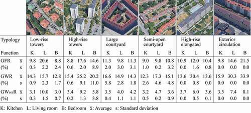
Building drawings were retrieved from the municipal archive of Malmö (Malmö-Stad 2020), were re-drawn in CAD format and analyzed using Grasshopper (Grasshopper 2020) to deduct geometric attributes per room. Attributes included the glass-to-floor ratio (GFR), the glass-to-wall ratio (GWR) and the glass-to-internal wall ratio (GW_INTR), which is the ratio of the glazing area divided by the total interior walls area. The drawings were validated via on-site measurements taken in a sample of apartments (20% of apartments). It was found that the municipal archive drawings were up-to-date, except for a few cases with removed interior wall partitions. Figure 2 shows the six surveyed developments, along with means ($\bar{\mathrm{x}}$) and standard deviations (s) of the three geometric attributes per room function.

2.2. Survey period and subjects

The questionnaire was distributed on March 13, 2018, aiming for occupants to respond during a period close to the spring equinox. Indeed the vast majority of participants (90%) gave their responses between March 14 and March 28. Overall, 108 questionnaires were mailed back. Post-processing revealed that 28 were missing values while five questionnaires did not include all three room functions K, L, B (small apartments). The response rate was calculated to 13%, but it was confirmed that there was satisfactory variation in age and gender among participants (Fig. 3). Sufficient variation in age is important, as it is by far the most common cause of limited visual capacity (Boyce 2017), as well as an influencing factor of electric lighting use in Swedish residential spaces during the day (Zimmermann 2009).

Fig. 3. Percentage of participants per age group and gender

The main procedure used to provide a quantitative subjective evaluation of the rooms was semantic differential (SD) scales. Two SD scales were used for each room function as shown in Fig. 4 (EL & DA). A third item was included at the end of the questionnaire as a multiple-choice question with a single-answer option (PR). The reader may refer to the Supplemental Material for the complete questionnaire; this includes additional items that were used in a previous publication and are irrelevant to the present study. The EL item aimed to measure the frequency of electric lighting use during the daylight hours of the year (EL). The DA item aimed to measure the portion of the room area that is sufficiently daylit throughout the year. The PR item aimed to assess occupant preferences, in particular, which room would be tolerated without daylight if there had to be one such room. Due to missing EL and DA data in some questionnaires, the processed responses for EL and DA were 75 per room function (75 apartments, 225 rooms), and PR responses were 108 (108 apartments). During processing, the EL response was quantified with an index ranging from 1 = “never” to 7 = “always”, and similarly, the DA response from 1 = “none” to 7 = “all the area”, as shown indicatively below the scales in Fig. 4.

Fig. 4. Questionnaire items: i) EL, the self-reported frequency of daytime electric lighting use throughout the year, ii) DA, the perceived area portion that is adequately daylit over the year and iii) PR, the preferred room function to be underlit, if there had to be one

2.3. Questionnaire design

Previous work on semantic differential scales indicates that different participants may use the same scale to assess different aspects of the physical environment (Houser and Tiller, 2003). The design and formulation of items can influence responses (Lietz 2010). Tiller and Rea (1992) have previously advocated that ambiguous use of semantic differential scales can be prevented by adequately defining i) the response measure, and ii) the dimensions of the response. The items in Fig. 4 were formulated accordingly, in order for every participant to assess the same aspect of the environment, with the same measurement scale.

2.3.1. Definition of response measure

On a basic level, the participant is required to know the semantic meaning of the words used in the items. On a higher level, the aspect to be assessed should be comprehended. In the case of the EL item, the clause “you turn on electric lighting” is a clear concept. The term “how often” can be intuitively understood as a measure of frequency. Observing the extreme adverbs of frequency at the ends of the response scale (never, always) facilitates understanding. The reference period was the daylight hours of the year. To avoid confusion of the term “daytime” with a potential working schedule (e.g. 8:00– 17:00), the underlined clause “when the sun is above the horizon” was used instead (Fig. 4). In the case of the DA item, two segments of the question needed to be salient: the part “how much of the … area” that refers to an area measure and the part “enough daylight” that refers to preferred daylight levels. When in the context of rooms, the Swedish word used for the term “area” (yta) is semantically connected to the “floor area”, i.e. refers to a region on the horizontal plane whose boundaries are defined by the room walls. The Swedish words used for “how much of” (the area) were “hur stor del av” (yta), the literal translation being “how big part of” (the area), which inherently refers to a portion of area, a fraction of the total space. The term “all the area” at the right end of the scale further clarifies this. The Swedish term used for “enough”, “tillräckligt med”, is the generic term for “sufficient amount of” or “adequate amount of”. In conjunction with “daylight”, it connotes daylight sufficiency in order to conduct a task (e.g. reading, cooking, etc.). “Tillräckligt med dagsljus” (enough daylight) is the official terminology used by Boverket, the state authority that issues Swedish building regulations, to refer to adequate amounts of daylight (BOVERKET 2020b).

2.3.2. Definition of response dimensions

To ensure that the response magnitude was measured consistently by participants, it was important that the terms at the ends of the scales were bipolar opposites that could define the entire range of possible measures. The two terms at the sides of each scale were also equidistant from the neutral central point (rating 4). The EL response was bounded by the terms “never” and “always”, as frequency is normally considered to vary along these two terms. For DA, the terms “none” and “all the area” were used, as they define all possible dimensions, ranging from the smallest possible to largest possible amount of room area.

2.3.3. Additional instructions for participants

A pilot study was conducted prior to collecting data, with nine subjects from the author’s work environment, to ensure that individual items operate well, but also to verify that the questionnaire as a whole was appropriately structured. Informal interviews with the nine participants indicated that the DA area was consistently understood as the area “satisfactorily lit” or “bright enough”. However, the extent of area under evaluation was unclear in cases where the kitchen was not separated from the dining room or the living room by a wall partition. Therefore, additional instructions were included per room function, as shown in the questionnaire found in the Supplemental Material. For instance, the kitchen items were preceded by the clarification: “The ‘kitchen’ is considered the area around the kitchen cabinets. A dining area away from the kitchen cabinets should not be considered for the following questions”. For the living room, it was clarified that “If the apartment has one kitchen and only one other room, then that room should be considered the ‘living room’ ”. This instruction was included to guide participants living in apartments that did not have a separate bedroom, i.e. sleeping occurs in the same space as the living room activities (small apartments). However, the present study did not assess any such apartment. Finally, for the bedroom, it was clarified that “If the apartment has more than one bedrooms, then answer the following questions ONLY for the largest bedroom”. There were two reasons for this decision. The first reason was that in case of multiple bedrooms, the largest bedroom (main bedroom) was expected to correspond to the main tenant of the apartment, for instance to the parent instead of the child, who was also expected to be the responder. The second reason was that the room would need to be identified (among other bedrooms) on the plan of the apartment during post processing (Fig. 1-iv, Locating participants). In the following sections of this paper, the term “bedroom” stands for “the main bedroom”, i.e. the largest bedroom in the apartment.

2.3.4. Retrieval from memory

Both EL and DA items ask retrospective questions, i.e. they refer to a period preceding the survey. The EL item asks participants to construct an estimate of absolute frequency, which is meant to characterize lighting use throughout the year. In other words, participants have to reflect on past behavior within a long period to provide a response. The response accuracy is thus dependent on the ability to retrieve memories, which means that noise can be expected. However, three factors in this study design may improve the accuracy in this estimate. Firstly, electric lighting use is repeated on a daily basis, as a habitual task, which facilitates memorization. Secondly, there are cues connected to this habit such as domestic tasks (e.g. cooking at specific times) or room occupancy patterns (e.g. being in specific rooms at specific times). The association with such cues in the environment facilitates the retrieval of long-term memories through so-called retrieval cues (Goldstein 2014). Retrieval is further facilitated by the fact that responding takes place in the same room as the room where the habit takes place, which can yield context-dependent retrieval (Godden and Baddeley 1975). Thirdly, the survey was conducted during a period that represents “average” daylight conditions (spring equinox). This effectively means that even if a participant were to base his or her answer on recent behavior to provide a response (e.g. within two weeks prior to the survey), this behavior would be during a period of typical daylight availability and average daytime duration with respect to the entire year. The same factors (i.e. cues, context, and time of survey) facilitate responding to the DA item, with the difference that the response relies on retrieving memories of the space, instead of memories of behavior in it.

2.3.5. Inattentive responding

Inattentive responding, also known as careless responding, refers to participants responding to items without regard to what is actually being asked. Meade and Craig (2012) have identified four factors affecting careless responding: respondent interest, survey length, social contact and environmental distraction. Inattentive responses can also be expected from occupants who have no prior experience upon which to base their response (Fotios 2019), for instance tenants that moved recently into the apartment and have not lived there long enough to make an informed estimate. Several strategies were used to alleviate inattentive responding. There was an introductory page explaining the importance of daylight and the significance of the collected data, i.e. potential influence on policy making. The latter was also meant to instill a sense of responsibility for the answers provided. The overall questionnaire length was kept to a minimum (two pages) to avoid attention waning over the course of a lengthy process. The fact that participation was voluntary was stated twice, in order to avoid a sense of obligation to participate. There was also no monetary incentive (or other form of retribution), which could potentially motivate a person to participate regardless of lacking knowledge or experience upon which to base his or her response.

2.3.6. Context effects

Literature on survey context effects has previously shown that preceding items can affect responses to subsequent items (Strack and Martin 1987). This could happen in two cases in this study: i) a response for the first room appearing in the questionnaire could affect a response for the following room and ii) the EL response could affect the DA response for a given room. To avoid the first case, the EL and DA items for each room function (kitchen, living room and bedroom) were placed in separate sections of the questionnaire. These sections were separated from each other by distinct headings, instructions and visual markers. They were also separated by seven additional items and fill-in instructions per room, and the occupant was asked to enter each room prior to responding to items for it (see Supplemental Material for complete questionnaire). Effects between the EL and DA items were alleviated by formulating questions to refer to different contexts. The EL item asks for a response on previous behavior (activity of turning lights on, “how often”), while the DA item refers to previous visual perception (experience of space, “how big an area”). In addition, different formulations were used for the reference period (EL: “when the sun is above the horizon”, DA: “during the year”). These differences along with a salient definition of each item ensure understanding of each response measure and prevent the two items from being perceived as parts of the same context or sequence (whole – part), alleviating assimilation and contrast effects (Schwarz et al. 1991; Tourangeau and Rasinski 1988).

2.3.7. The preference item PR

The third item in Fig. 4 regarded occupant preferences (PR), in particular, which room would be tolerated without daylight, if there had to be one such room. This item aimed at revealing (if any) popular prioritization with respect to daylight availability. This prioritization may be useful in devising design guidelines, considering constraints pertaining to multi-dwelling buildings as opposed to single-family (detached) houses. For instance, there is a high probability that a room is placed deeper into the building core and away from the exterior wall if facades are not extensive enough to arrange all rooms along the perimeter of the building (deep plan buildings). There is also no possibility to utilize skylights for rooms far from the façade, except in apartments on the top floor. The first three choices for the PR response corresponded to the three room functions. A fourth choice was given as an option, (response: “I don’t know which one”). This response includes all those occupants that cannot make a clear distinction, due to any of the following three reasons: i) because they value daylight equally for all functions, ii) because they would not accept any room being underlit, iii) because the room they would choose was not included in the questionnaire (e.g. bathroom).

2.4. Types of electric lighting use

Electric lighting use in each room was assigned a specific “type”, based on the relation between the EL and DA responses. In essence, the concept of categorizing electric lighting use into different “types” was based on whether or not the user responds to available daylight levels by using electric lighting accordingly. The Euclidean distances between responses EL, DA and the scale midpoint (rating = 4) were calculated to define five types of use (Table 1). The use was assumed responsive when the EL response was the reverse of the DA response with respect to the scale midpoint (EL = 8 – DA), namely: 1v7, 2v6, 3v5, 4v4, 5v3, 6v2, 7v1. This type characterizes electric lighting use that is responsive to daylight availability, i.e. the lighting switch-on behavior corresponds to daylight levels. If electric lighting is normally off in a very bright space, this is considered responsive by the study. The latter implies that responsive use is not determined by the degree of electric lighting use, but by its association with perceived daylit area (DA). The second type of use, termed responsive ±1, was assigned when responses deviated from responsive by a distance of ± 1 on the rating scale (EL = (8 – DA) ±1), for instance 1v6 instead of 1v7, 2v7 instead of 2v6 etc. Similarly, the responsive ±2 use was assigned when responses deviated from responsive by a distance of ± 2 on the rating scale (EL = (8 – DA) ±2). The three aforementioned types of use (responsive types) did not include rooms with both responses greater than 4 or both lower than 4. In other words, responsive types of use are characterized by a negative correlation between EL and DA. On the contrary, the fourth and fifth types included combinations where EL and DA were positively correlated. More specifically, the fourth group included rooms where occupants reported higher frequencies of electric lighting use and larger extents of daylit area. The use in these rooms was considered irresponsive, since electric lighting is used despite the large extent of the daylit area (EL ≥ 4 and DA ≥ 4, excluding the pair with EL = DA = 4). This type was termed irresponsive EL↑-DA↑. On the other hand, in some cases electric lighting use was reported as infrequent although only a small daylit area was reported. The electric lighting use in these rooms was termed irresponsive EL↓-DA↓ (EL ≤ 4 and DA ≤ 4, excluding the pair with EL = DA = 4), i.e. EL is low despite DA being low.

Table 1. Combinations of EL and DA responses for each type of use (49 in total)

Type of use	responsive	responsive ±1	responsive ±2	irresponsive EL↑-DA↑	irresponsive EL↓-DA↓
(EL, DA)	(1,7)	(1,6)	(1,5)	(4,7)	(1,4)
	(2,6)	(2,7)	(3,7)	(4,6)	(1,3)
	(3,5)	(2,5)	(5,1)	(4,5)	(1,2)
	(4,4)	(3,6)	(7,3)	(5,7)	(1,1)
	(5,3)	(5,2)		(5,6)	(2,4)
	(6,2)	(6,3)		(5,5)	(2,3)
	(7,1)	(6,1)		(5,4)	(2,2)
		(7,2)		(6,7)	(2,1)
				(6,6)	(3,4)
				(6,5)	(3,3)
				(6,4)	(3,2)
				(7,7)	(3,1)
				(7,6)	(4,3)
				(7,5)	(4,2)
				(7,4)	(4,1)
Combinations	7	8	4	15	15

2.5. Evaluated room groups

The EL and DA responses were analyzed considering the overall room sample (S_ALL, N = 225), and groups extracted from it according to room function, occupant age, balcony obstruction, orientation, geometry and type of electric lighting use. The sizes of different groups are shown further down in the Results section to avoid repetition here. With respect to room function, there were three groups K, L, B, one per function (K: kitchen, L: living room and B: bedroom). With respect to age, rooms were divided into six groups according to ranges “< 30”, “(30– 39)”, “(40– 49)”, “(50– 59)”, “(60– 69)” and “≥ 70”. With respect to balcony, rooms were divided into two groups, one group including rooms with a balcony obstruction above their fenestration, and one without (YES, NO, respectively). These groups only included rooms where the balcony obstructed all available fenestration area in order to assess the balcony impact, thus 196 out of 225 rooms were included. In terms of orientation, rooms were divided into groups N, W, S, E corresponding to North-facing, West-facing, South-facing and East-facing rooms respectively. The rationale for grouping rooms according to orientation was the azimuth angle of the room’s fenestration normal, measured clockwise starting from North. Four distinct angular ranges were defined based on the mid-cardinal compass points, e.g. a room was considered East-facing for a façade normal direction between angles 45° and 135°, South-facing for a façade normal direction between angles 135° and 225° etc. In terms of geometry, rooms were dichotomized into two groups for each of the geometric attributes GFR, GWR, GW_INTR, one group including rooms with the lowest half of the attribute values and one group including rooms with the highest half. The comparison between low and high attribute groups were performed separately for each room function, as paired samples t-tests comparing GFR, GWR and GW_INTR between the K, L, B groups revealed significant differences between function groups for all geometric attributes. Finally, seven groups of rooms were defined according to type of electric lighting use: i. responsive (only rooms with responsive use), ii. responsive ±1 (only rooms with responsive ±1 use), iii. responsive ±2 (only rooms with responsive ±2 use), iv. irresponsive EL↑-DA↑ (only rooms with irresponsive EL↑-DA↑ use), v. irresponsive EL↓-DA↓ (only rooms with irresponsive EL↓-DA↓ use), vi. responsive OR responsive ±1 (rooms with either responsive or responsive ±1 use) and vii. irresponsive EL↑-DA↑ OR irresponsive EL↓-DA↓ (rooms with either irresponsive EL↑-DA↑ or irresponsive EL↓-DA↓ use). It should be noted here that the combined group responsive OR responsive ±1 was used in specific statistical tests with the aim to evaluate whether it is usual for EL and DA to be strongly associated across rooms of specific groups (e.g. kitchens, North-facing rooms, ages (30– 39) etc.), in particular negatively associated. Type responsive ±2 was not included in this combined group, even though it too refers to a negative association between EL and DA. The reason is that it refers to a weaker association (Table 1). In essence, testing for a significant frequency of responsive OR responsive ±1 rooms in a group yields more statistical power for the analysis with respect to the EL and DA association effect, in comparison with testing for the frequency of responsive OR responsive ±1 OR responsive ±2 rooms.

2.6. Data analysis

2.6.1. Association between EL and DA

The Spearman rank correlation coefficient r_S was used to measure the strength of association between EL and DA. The choice over Pearson’s correlation was made since r_S is preferable in heavy-tailed distributions or when outliers are present (de Winter et al. 2016), which was the case with multiple room groups in this study. The association strength was interpreted according to the three-tier effect size categorization suggested by Cohen (Cohen 1988), where the effect size is considered small for an absolute value of r_S lower than 0.3, medium for an absolute value of r_S between 0.3 and 0.5, and large for an absolute value of r_S greater than 0.5. Post-hoc analysis using G*Power (Faul et al. 2007) revealed that the sizes of all groups and corresponding effect sizes r_S ensured the conventional statistical power threshold of 0.8 for a significance level p < .05.

2.6.2. Difference between associations

Pairwise comparisons between group correlation coefficients (r_S1 vs r_S2) were performed, to evaluate whether the EL and DA association is stronger in certain room groups. The procedure involved constructing the 95% confidence interval for the r_S difference between a given pair of groups. The confidence interval construction approach can reveal both the precision and magnitude of an effect, as opposed to significance testing using a-priori hypotheses, which is why it is preferred over typical significance tests in the context of correlations (Olkin and Finn 1995). For a given pair of groups 1 and 2 with correlation coefficients r_S1 and r_S2, the procedure included constructing the confidence interval for the r_S1 – r_S2 difference (CI_{1_2}: [L, U]) according to Zou (2007). The difference between r_S1 and r_S2 was not considered statistically significant if CI_{1_2} contained zero. Zou (2007) provides different formulae to calculate CI_{1_2} for independent and dependent (paired) groups; the suitable calculation was used depending on the groups compared. In the case of orientation groups N, W, S, E, and balcony groups YES, NO, the pairs of groups (e.g. S vs E, or YES vs NO) were only partially paired, i.e. one portion of participants was included in both groups, and one portion of participants was included in only one of the two groups (either one). In these cases, responses were removed from the largest group randomly (with equal probability of removal), with the intent to acquire two independent groups with the highest possible size for the smaller group. Subsequently, the confidence interval for the r_S1 – r_S2 difference was constructed according to the formulae suitable for independent groups.

2.6.3. Analysis of electric lighting use types

The percentage of rooms with a specific type of electric lighting use was calculated in each group. To compare percentages, one variable with two categories (1, 0) was created per type of use, where 1 indicates that the room is characterized by the type and 0 that it is characterized by any other type. Binomial tests (Glass and Hopkins 1995) were performed to assess if the percentage was significantly higher or lower than the percentage expected from random responses. If the EL and DA responses were randomly selected by each participant, the probability of occurrence for a given type would depend on the number of combinations shown in Table 1 (responsive: 7/49 = 0.14, responsive ±1: 8/49 = 0.16, responsive ±2: 4/49 = 0.08, irresponsive EL↑-DA↑: 15/49 = 0.31 and irresponsive EL↓-DA↓: 15/49 = 0.31). Similarly, for responsive OR responsive ±1 the expected probability would be equal to (7 + 8)/49 = 0.31. Binomial tests where used to assess the statistical significance of deviations from these expected distributions (e.g. expected distribution for responsive use is 14% for 1, and 86% for 0). A significant test result indicated that the percentage of rooms with a given type of use was significantly high or low. The alpha level considered was α = 0.05 (2-tailed).

Two different tests were used to compare groups, depending on group relation. McNemar tests were used for paired groups, namely the function groups (K, L, B), and Chi-square tests were used to compare independent groups, which included all other groups. The McNemar test can be used to compare percentages (e.g. percentages of responsive rooms) for two paired groups (e.g. KvL), and is suitable for non-parametric binary data (McNemar 1947). The test is applied to a 2 × 2 contingency table and is calculated based only on the number of subjects who gave different responses per group (discordant pairs of responses), for instance, a discordant pair of responses from the same subject could be: ‘K: responsive = 0, L: responsive = 1ʹ. Subjects that gave the same response for both groups (concordant pairs) are not accounted for by the test. The probability (p-value) of the test is based on discordant pairs, and the way it is calculated depends on their number. The test statistic has a chi-square distribution, but if the number of discordant pairs is less than 25, the statistic is better approximated by the binomial distribution. Previous research supports that this renders the test more conservative, and that a mid-p value (calculated p-value divided by 2) should be used in such cases (Fagerland et al. 2013); the mid-p value was used in this study wherever applicable as per the aforementioned suggestion. Finally, the Odds ratio (OR) was calculated to assess the effect size of the test (Cleophas and Zwinderman 2016), since the McNemar test only assesses significance.

The Chi-square test of independence was used to compare age, orientation and balcony groups. Specifically for this test, the six age groups were merged into two groups, one for all participants aged below 50 (< 50) and one for those aged 50 or higher (≥ 50). The Chi-square test of independence is designed to analyze group differences (e.g. South-facing vs North-facing rooms) when the dependent variable is measured at the nominal level (e.g. responsive = 1 or 0). It is robust with respect to the distribution of the data, i.e. it does not require equal variances among groups or homoscedasticity. As with McNemar’s test, it is also applied on a contingency table, in this study a 2 × 2 table. In cases where at least one table cell has an expected count less than 5, Fischer’s exact test can be used to compute the Chi-square test’s probability (Fisher 1922). The test only assesses the significance of the group difference, thus it should be followed by a strength statistic (McHugh 2013). The strength statistic used was Cramer’s V (Elliot et al. 2016), which ranges from 0, if the groups are independent of the variable, to 1, if the groups are perfectly predictive of the variable value, e.g. if room function is predictive of percentage of responsive rooms. According to Cohen (1988), Cramer’s V for a 2 × 2 contingency table corresponds to a weak, medium or large effect when equal to 0.1, 0.3 or 0.5 respectively.

2.6.4. Analysis of PR responses

The proportion of PR responses (responses for a preferred underlit room, if there had to be one) was calculated per category, namely for categories “kitchen”, “living room”, “bedroom” and “I don’t know which one” (Fig. 4). A Chi-square goodness-of-fit test was performed to evaluate if the categories were equally distributed (25% of responses per category), followed by Binomial tests per category to evaluate which one had a proportion significantly higher or lower than 25%. In addition, for those participants that age data were available (n = 76), binomial tests were performed to test the same assumption in each age group, i.e. which category of the PR response had a significantly different proportion than 25%, within different age groups.

3. Results

3.1. Association between EL and DA responses

The Spearman rank correlation between EL and DA responses for different groups is shown in Table 2. There is a significant negative association (p < .05) for all groups. Overall, the size of the association is large (All rooms: r_S = −0.588, p < .01), and ranges from medium-to-large to large across different groups (−0.4 ≤ r_S ≤ −0.8). The association was not significantly different between room functions as per the confidence interval of the r_S difference (CI_{K_L}: [−0.14, 0.24], CI_{K_B}: [−0.24, 0.16], CI_{L_B}: [−0.27, 0.09], p < .01). With respect to age groups, the strongest associations were found for groups “< 30”, “(40– 49)” and “≥ 70” (r_S = 0.-0.772, −0.767 and −0.746 respectively). All three were significantly higher than the association in the (50– 59) age group, but the confidence intervals of r_S differences were wide (CI_{<30_50-60}: [−0.66, −0.03], CI_{40-50_50-60}: [−0.65, −0.06], CI_{≥70_50-60}: [−0.63, −0.06]). When comparing between younger (age < 50) and older (age ≥ 50) participants, no significant difference was found. With respect to orientation, the North and South-facing rooms exhibit a medium-to-large effect (N: r_S = −0.405, S: r_S = −0.395, p < .05), while West and East-facing rooms exhibit a large and more significant effect (W: r_S = −0.582, E: r_S = −0.726, p < .01). Significant differences between associations were identified between East and North (CI_{E_N}: [−0.66, −0.04]) and between East and South (CI_{E_S}: [−0.65, −0.05]). In other words, the association between EL and DA was significantly higher in East-facing rooms compared to North and South-facing rooms (p < .05). Finally, the association is strong both for rooms with and without a balcony obstruction (YES: r_S = −0.576, NO: r_S = −0.550, p < .01), without a significant difference between the two groups (CI_{YES_NO} [−0.33, 0.20]).

Table 2. Spearman rank correlation coefficient r_S for overall sample S_ALL (n = 225), and for groups according to function, age, orientation and balcony obstruction

Variable	Group	n	rS
All rooms	SALL	225	−0.588**
Function	K	75	−0.570**
	L	75	−0.617**
	B	75	−0.531**
Age	< 30	21	−0.772**
	(30– 39)	45	−0.478**
	(40– 49)	30	−0.767**
	(50– 59)	48	−0.408**
	(60– 69)	33	−0.633**
	≥ 70	42	−0.746**
Orientation	N	35	−0.405*
	W	85	−0.582**
	S	38	−0.395*
	E	67	−0.726**
Balcony^a	NO	155	−0.550**
	YES	41	−0.576**

*, ** significance p < .05, p < .01 respectively

^aonly includes single-aspect rooms

The effect of geometric attributes on r_S was evaluated separately in each function group K, L, B, since paired samples t-tests indicated that these attributes differ significantly between groups (p < .05). Table 3 shows the association for different ranges of attributes and different orientations. Cases where r_S was significantly different between two groups are marked with “*”. It is shown that there is a negative association (p < .05) for the majority of groups. Wherever significant, the association effect ranges between −0.429 and −0.804. This indicates that the stratification of rooms based on function and geometry did not yield different results compared to Table 2. In the case of living rooms, two geometric attributes yield a markedly different association depending on their range. The association is significantly stronger for living rooms with higher GFR (r_{S_13.8–25.3} = −0.754) compared to lower GFR (r_{S_0-13.8} = −0.443), CI_{0-13.8_13.8–25.3}: [0.02, 0.65], and for living rooms with higher GW_INTR (r_{S_6.7–13.2} = −0.773) compared to lower GW_INTR (r_{S_0-6.7} = −0.436), CI_{0-6.7_6.7–13.2}: [0.05, 0.67]. In essence, the lower range geometry values correspond to single-aspect living rooms, while the higher range values correspond to multi-aspect living rooms. It should be noted that age, orientation and balcony categories were equally represented among these pairs of groups. Finally, with respect to orientation, the association is strong in kitchens and living rooms oriented toward East or West (0.623 ≤ |r_S| ≤ 0.714, p < .01), and in bedrooms oriented toward East or South (East: r_S = −0.804, p < .01, South: r_S = −0.625, p < .05). However, post-hoc analysis indicated that there is no statistical power for r_S in the rest of the groups, i.e. the possibility that there is an association between EL and DA cannot be ruled out for them.

Table 3. Spearman rank correlation coefficient r_S per room function, within different ranges of GFR, GWR, GW_INTR, and different orientations

	Kitchen			Living room			Bedroom
Variable	Group	n	rS	Group	n	rS	Group	n	rS
GFR	(0– 9.81)	37	−0.513**	⋆(0– 13.79)	34	−0.443**	(0– 10.9)	39	−0.540**
	(9.82– 15.4)	38	−0.623**	⋆(13.8– 25.3)	41	−0.754**	(11.0– 24.6)	36	−0.528**
GWR	(0– 14.69)	36	−0.547**	(0– 16.99)	36	−0.564**	(0– 13.99)	36	−0.633**
	(14.7– 27.7)	39	−0.618**	(17– 32)	39	−0.613**	(14– 33.9)	39	−0.429**
GWINTR	(0– 3.4)	34	−0.618**	⋆(0– 6.69)	35	−0.436**	(0– 3.79)	37	−0.542**
	(3.5– 4.3)	41	−0.529**	⋆(6.7– 13.2)	40	−0.773**	(3.8– 10.1)	38	−0.529**
Orientation	N	5	−0.649	N	13	−0.318	N	18	−0.402
	W	29	−0.623**	W	32	−0.714**	W	23	−0.166
	S	13	−0.088	S	12	−0.405	S	13	−0.625*
	E	28	−0.675**	E	18	−0.644**	E	21	−0.804**

*, ** significance p < .05, p < .01 respectively

⋆ significant difference between two correlations

3.2. Type of electric lighting use

Table 4 shows the percentage of rooms in each group that have responsive, responsive ± 1, responsive ± 2, responsive OR responsive ± 1, irresponsive EL↑-DA↑ or irresponsive EL↓-DA↓ lighting use. Markers (+) and (-) indicate that a percentage is significantly higher or lower than what would be expected from random responses (Binomial test). The first row of the table confirms that there is an association between EL and DA. For the overall sample (All rooms), the percentage of rooms with either a perfect or a nearly perfect negative association between EL and DA (column responsive OR responsive ±1) is 73%. The percentage was found significantly higher (+) than what would be expected from random responses (15%). Rooms characterized by responsive, responsive ± 1 and responsive ± 2 correspond to 38%, 36% and 6% of the overall sample (respectively). The percentages of rooms with irresponsive EL↑-DA↑ and irresponsive EL↓-DA↓ electric lighting use were found significantly low (All rooms, irresponsive EL↑-DA↑: 10%, irresponsive EL↓-DA↓: 10%, (-)).

Table 4. Percentage of rooms per group with a given electric lighting use type. Markers (+) and (-) indicate that a percentage is significantly higher or lower (respectively) than what was expected (Binomial test)

Variable	Group	n	responsive (%)	responsive ±1 (%)	responsive ±2 (%)	responsive OR responsive ±1 (%)	irresponsive EL↑-DA↑ (%)	irresponsive EL↓-DA↓(%)
All rooms	SALL	225	38 (+)	36 (+)	6	73 (+)	10 (-)	10 (-)
Function	K	75	29 (+)	36 (+)	8	65 (+)	16 (-)	11 (-)
	L	75	48 (+)	32 (+)	5	80 (+)	5 (-)	8 (-)
	B	75	36 (+)	39 (+)	5	75 (+)	9 (-)	9 (-)
Age	< 30	21	48 (+)	24	5	71 (+)	24	0 (-)
	(30– 39)	45	20	47 (+)	2	67 (+)	20	11 (-)
	(40– 49)	30	40 (+)	47 (+)	0	87 (+)	10 (-)	3 (-)
	(50– 59)	48	35 (+)	27	8	62 (+)	13 (-)	17
	(60– 69)	33	42 (+)	36 (+)	18	79 (+)	0 (-)	3 (-)
	≥ 70	42	48 (+)	33 (+)	5	81 (+)	0 (-)	14
Orientation	N	35	36 (+)	28 (+)	8	64 (+)	11 (-)	17
	W	85	43 (+)	39 (+)	4	82 (+)	7 (-)	7 (-)
	S	38	32 (+)	34 (+)	3	66 (+)	18	13
	E	67	36 (+)	36 (+)	10	72 (+)	9 (-)	9 (-)
Balcony^a	NO	155	38 (+)	35 (+)	5	73 (+)	11 (-)	12 (-)
	YES	41	29	41 (+)	12	71 (+)	10 (-)	7 (-)

(+), (-) significantly higher or lower than expected (Binomial test).

^aonly includes singe-aspect rooms

Observing Table 4, it is shown that the percentage of responsive OR responsive ± 1 is significantly high across all groups (all percentages (+)). In addition, for the majority of groups, there were significantly few rooms with irresponsive EL↑-DA↑ or irresponsive EL↓-DA↓ use (most percentages (-)). Exceptions for irresponsive EL↑-DA↑ use include the two lower age groups (<30: 24%, (30– 39): 20%), and South-facing rooms (S: 18%). Exceptions for irresponsive EL↓-DA↓ use include age groups (50– 59) and ≥70 (irresponsive EL↓-DA↓: 17% and 14% respectively), as well as North-facing and South-facing rooms (irresponsive EL↓-DA↓: 17% and 13% respectively). Overall, frequent responsive OR responsive±1 use persists across groups of different characteristics. The percentage of irresponsive EL↑-DA↑ rooms are significantly low for all groups, while the percentage of irresponsive EL↓-DA↓ rooms are significantly low for most groups (in 11 out of 15 groups).

With respect to differences between groups K, L, B, the McNemar test result was statistically significant in three cases, all of which correspond to the comparison between K and L. The percentages of responsive and responsive OR responsive ±1 were significantly higher in living rooms compared to kitchens (responsive: p = .003, OR = 3.8, responsive OR responsive ±1: p = .017, OR = 2.83), and the percentage of irresponsive EL↑-DA↑ rooms was significantly higher in kitchens compared to living rooms (irresponsive EL↑-DA↑: p = .019, OR = 5.0). There were no other significant differences between function groups. With respect to age group comparisons, the Chi-square tests revealed one significant difference. Participants aged 50 or higher reported irresponsive EL↑-DA↑ use significantly less frequently than participants aged below 50 (χ²(1) = 9.443, p = .002), but the magnitude of the difference was weak-to-medium (Cramer’s V = 0.21, p < .01). With respect to orientation group comparisons, the Chi-square tests revealed two significant differences, both regarding responsive OR responsive ±1 use. This type of use was reported more frequently in West-facing rooms compared to North-facing rooms (x2(1) = 5.896, p =.015), with a weak-to-medium effect size (Cramer’s V = 0.227, p = .015), and more frequently in West-facing rooms compared to South-facing rooms (x2(1) = 4.055, p =.044), with a weak-to-medium effect size (Cramer’s V = 0.391, p = .026). Finally, no significant differences were identified between balcony groups NO, YES for any type of use.

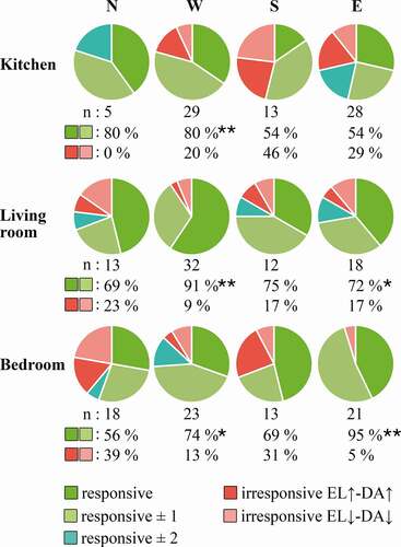
Each pie chart in Fig. 5 corresponds to a subgroup including rooms of a specific function (kitchen, living room or bedroom) oriented toward a particular orientation (N, W, S, E). Each slice corresponds to the percentage of rooms in the subgroup that are characterized by a given type of electric lighting use (responsive, responsive ±1, etc.). Cumulative percentages are shown below each pie chart for responsive OR responsive ± 1 rooms (green hues) and irresponsive EL↑-DA↑ OR irresponsive EL↓-DA↓ rooms (red hues), which correspond to proportions of rooms with a negative and positive association between EL and DA respectively (green hues: negative, red hues: positive). It is shown that the green hue prevails, i.e. lighting use is responsive OR responsive ± 1 for the majority of rooms in each subgroup (> 50% of rooms). Binomial tests indicated that the proportion of responsive OR responsive ± 1 rooms is significantly higher than 50% in i) West-facing kitchens (90%, p < .01), ii) West and East-facing living rooms (91%, p < .01 and 72%, p < .05 respectively) and in iii) West and East-facing bedrooms (74%, p < .05 and 95%, p < .01 respectively). Comparing orientations for each room function, one significant difference was revealed. West-facing kitchens reported responsive OR responsive ± 1 use more frequently compared to East-facing kitchens (χ²(1) = 4.247, p = .039), with a medium effect size (Cramer’s V = 0.273, p < .05). Two more comparisons had marginally significant results (p < .1). Living rooms oriented toward West reported responsive OR responsive ± 1 use more frequently than living rooms oriented toward East (χ²(1) = 3.075, p = .091, Cramer’s V = 0.273, p = .079), and bedrooms oriented toward East reported responsive OR responsive ± 1 use more frequently than bedrooms oriented toward West (χ²(1) = 3.731, p = .062, Cramer’s V = 0.291, p = .053). This information indicates that West orientation is favorable for kitchens and living rooms, while East is favorable for bedrooms, which is in line with the r_S magnitude shown in Table 3 for the orientation groups; however, larger room samples are required to corroborate this finding.

Fig. 5. Proportion of each type of electric lighting use per orientation and room function. Cumulative percentages are shown for responsive OR responsive ± 1 rooms (green hues), and for irresponsive EL↑-DA↑ OR irresponsive EL↓-DA↓ rooms (red hues). The number of rooms per function and orientation is indicated by “n”. Markers “*” and “**” indicate significance at 0.05 and 0.01 respectively, for Binomial tests with an expected proportion of 50%

3.3. Daylight prioritization per room function

Figure 6 shows the percentage of responses in each PR category for a sample of 108 participants. These are responses to the question “If any of the rooms would be without daylight, which one would you choose?”. Percentages that correspond to significant Binomial test results are marked with “*”. It is shown that the bedroom is the space where most occupants would tolerate low daylight levels, if they had to choose one such room (62.0% of the occupants). The second most chosen category, and more frequent than the remaining two choices, is the “I don’t know which one” category (25.0%). The “Living room” responses were few (8.3%), and “Kitchen” responses were extremely few (4.6%). This indicates that the kitchen is the space within the apartment where the vast majority of participants would not tolerate the lack of daylight (only 5 out of 108 chose “Kitchen”). The Chi-square goodness of fit test for an expected percentage of 25% per category was significant, χ²(3) = 89.19, p < .01. The result was followed by individual Binomial tests per category. It appeared that the percentages of “Kitchen” and “Living room” responses were significantly lower than 25% (Kitchen: 4.6%, Living room: 8.3%, p < .01 for both), and the percentage of “Bedroom” responses was significantly higher (62.0%, p < .01). The percentage of participants who chose category “I don’t know which one” was exactly 25% (27 out of 108 responses).

Fig. 6. Percentage of PR responses per category. The PR responses were given for the question: “If any of the rooms would be without daylight, which one would you choose” (Fig. 4). Indicated with “**” are percentages significantly higher or lower than 25%, as per the Binomial test results

Figure 7 shows the percentage of PR responses that correspond to each room function, per age group. Percentages that are significantly higher or lower than 25% (as per the Binomial tests (p < .05)), are marked with “(+)” and “(-)”. The numerals below the age ranges at the x-axis show the percentage of responses that were either “Bedroom” or “I don’t know which one”, i.e. the percentage of participants that did not choose neither the “Kitchen” nor the “Living room” category. These percentages are marked with “*” and “**” when significantly higher than 50%, as per the Chi-square goodness-of-fit test (p < .05, p < .01 respectively). It is shown that the “Bedroom” category was chosen most frequently and the “I don’t know which one” was the second most chosen category, in all groups except for the “≥ 70” group where the two categories have the same proportion (43% each). This is the only group where the majority of participants did not choose “Bedroom”. For this group, the “Bedroom” percentage (43%) is not significantly higher than 25%, which is the expected percentage if all categories where considered equally probable. For the rest of the groups, the “Bedroom” response is significantly more frequent than 25%. Overall, the percentage of participants who did not choose neither “Kitchen” nor “Living room” deviated significantly from 50%, as indicated consistently by the percentages shown below the x-axis (“Bedroom” OR “I don’t know which one” percentages between 86% and 100%). A significant result was not obtained for the “< 30” group due to low group size (n = 7).

Fig. 7. Percentage of PR responses per room function and age group. Significantly high or low percentages are marked with (+) or (-) respectively. The x-axis also shows the cumulative percentage of responses “Bedroom” or “I don’t know which one”. The percentages are marked with “*” and “**” when significantly higher than 50%, as per the Chi-square goodness-of-fit test (p < .05, p < .01 respectively)

Figures 8 and 9 juxtaposed with Fig. 6 can help illustrate a contradiction between reported electric lighting use and perceived daylit area on one hand (EL & DA), and preferences with respect to daylight availability on the other hand (PR). Figure 8 suggests that daytime electric lighting use is more frequent in kitchens, as nearly one out of three kitchens uses electric lighting more often than half the daylight hours in a year (EL ≥ 5 in 32% of the rooms). McNemar tests indicated that the percentage of kitchens was significantly higher than that of living rooms (p = .004, OR = 5) and significantly higher than that of bedrooms (p = .021, OR = 3). In addition, Fig. 9 shows that kitchens were reported underlit (DA ≤ 3) more often than the other two room functions. In particular, nearly one out of four occupants reported a low daylit area in their kitchen (DA ≤ 3, K: 24%), while the corresponding percentages for living rooms and bedrooms were 14.7% and 16.0% respectively. The McNemar test result was marginally significant when comparing kitchens with living rooms (p = .059) and kitchens with bedrooms (p = .09). Interpreting the information provided by Figs. 6, 8 and 9 combined, we can infer that there is a need to ensure/improve daylight provision for kitchens. The latter is true since: i) very few occupants would tolerate an underlit kitchen (Fig. 6), the most frequent electric lighting use during daytime occurs in kitchens (Fig. 8) and iii) kitchens were most frequently reported as underlit (Fig. 9).

Fig. 8. Percentage of high-frequency electric lighting use (EL ≥ 5) responses, per room function

Fig. 9. Percentage of low daylit area responses (DA ≤ 3) per room function

4. Discussion

Reducing unnecessary electricity for lighting in the residential sector by means of daylight utilization is a laudable goal. As stated in the Introduction section, an increase of remote work (work-from-home) could induce an increase in residential electricity used for lighting; however, the net difference in electricity use would depend on the lighting power density [W/m2] of offices (where people left from) compared to residences (where people went to). The case might be that residences use less artificial lighting per unit area compared to offices, which would then result in less electricity use overall if people work from home. On the other hand, the lighting load per person should be factored in this comparison, as employees may share ambient lighting in e.g. open offices, while each employee would use a different luminaire if they worked from their individual home environment. Whatever the case, improving daylight performance to reduce electricity use for lighting in residences is a laudable goal, as it increases the resilience of these spaces and renders them more efficient as potential working spaces, if the need arises.

Daylight utilization in residences is also in phase with the need for integrative lighting (CIE 2016), which may produce both physiological and psychological benefits for humans. Although there are still gaps of knowledge regarding these benefits (Münch et al. 2020), there is evidence that timing the exposure to daylight radiation and increasing its quantity are very important (Figueiro 2017), and this is relevant specifically for residences. The reason is that residences are where people sleep, which makes their need for daylight in these spaces to vary with time: they require light with high melanopic content upon waking up and during the day, light with lower melanopic content before going to bed, and darkness when they sleep. This warrants the importance of daylight design for residences with respect to timing illumination for different rooms.

With respect to lighting use types, there are two considerations pertaining to their definition. Type irresponsive EL↑-DA↑ was assumed for rooms with frequent electric lighting use despite a large daylit area (EL, DA responses ≥ 4, excluding the 4v4 pair). The case could be that this type does not necessarily characterize an occupant who uses electric lighting regardless of daylight conditions. In cases of deep rooms, an occupant may use electric lighting at the back end of the room if the task is located there, although most of the room area may be adequately daylit. It appeared that there was only one living room with irresponsive EL↑-DA↑ use and designed with extensive depth (7.5 m), where a task could potentially be conducted in a dark location while most of the room area remains daylit. The most irresponsive EL↑-DA↑ rooms were kitchens (Table 4). Kitchens with irresponsive EL↑-DA↑ use had their counter on the side wall, the counter stretching throughout the room depth (4.5– 4.8 m). This depth was within the recommended range for daylit spaces (Reinhart 2005), and indeed these rooms were reported as having an extended daylit area (DA ≥ 5). In kitchens though, tasks of high contrast and small size such as cooking require higher levels of illuminance (DiLaura et al. 2011), probably higher than what would be perceived as adequate for the overall room area, which explains the higher percentage of irresponsive EL↑-DA↑ use in kitchens. The same spatial consideration applies for irresponsive EL↓-DA↓ electric lighting use. A person could potentially live in a room considered dark (DA ≤ 3), but still use electric lighting only on rare occasions (EL ≤ 3), e.g. if the task is located next to the window. Checking the apartment plans and survey photographs verified that this was not possible in kitchens or bedrooms. However, it could be possible in living rooms with a sitting area next to the window and the rest of the area stretching deep into the building core. This was possible in five out of six irresponsive EL↓-DA↓ living rooms, which indicates that the term irresponsive EL↓-DA↓ did not necessarily pertain to behavior characterized by indifference toward daylight conditions. If the latter is true, then these rooms could be considered similar to the rooms were EL and DA were negatively associated, further verifying the hypothesis of this study.

With respect to occupant preferences, it was shown that the majority of respondents (62%) would choose the bedroom as the underlit room of their apartment, if they had to choose one such room. This finding provides knowledge suitable for design guidelines. For instance, if one room or a percentage of the apartment area is predestined to be darker due to uncontrolled factors (e.g. high preexisting surrounding obstructions), it is preferable to accommodate a bedroom function in that space instead of a kitchen function. However, this prioritization should not affect children, which may be present in their bedroom earlier in the afternoon compared to their parents (Wolf 2020; Wolf et al. 2019). Daylight provision should also be considered in bedrooms for elderly people, as the “Bedroom” response did not stand out significantly in the “≥ 70” age group (Fig. 7). On the other hand, the kitchen was selected by a remarkably low amount of respondents (5 out of 108 respondents). Results indicated that this room function: i) would not be tolerated underlit, ii) was reported most often as using electric lighting frequently (EL ≥ 5) and iii) was reported most often as having a small daylit area (DA ≤ 3). It can therefore be inferred that daylight provision is needed for kitchens. The author has previously received skepticism for this conclusion, when presenting preliminary results in previous symposia or workshops, including comments from practitioners of architecture and policy makers in Sweden. The main point raised was that there is more necessity for daylight where one dines, compared to where one cooks, concluding that no daylight provision is necessary for the kitchen. Although this sounds like a reasonable argument, it is not supported by scientific evidence. The participants of this study were asked to exclude the dining area when responding for the kitchen, and still reported that they would not tolerate low daylight levels. This finding is in agreement with recently published work conducted in 45 Swedish apartments, where the kitchen was chosen as the most important room to have access to a lot of daylight, even though a choice was given to select the dining room instead (Eriksson et al. 2019, 21). In particular, the dining room only ranked third out of four room functions in terms of daylight prioritization, the kitchen being the most important, followed closely only by the living room, similarly what was found here (Fig. 6). The bedroom was voted as the least important room by a high margin, also similarly to the results presented here.

5. Conclusions

This paper presented results of a questionnaire survey in 75 apartments located in typical residential buildings in Malmö, Sweden, comprising 225 rooms that included kitchens, living rooms and bedrooms. The aim of the study was to assess if there is a potential to reduce residential electric lighting use by exploiting daylight, and to assess which rooms are prioritized with respect to daylight admission. The following may be concluded:

5.1. Associations between electric lighting use and daylit area

Overall, the size of the association between self-reported frequency of electric lighting use (EL) and perceived daylit area (DA) was found strong (r_S = −0.588, p < .01). The association was persistent through groups defined according to function, occupant age, orientation, balcony obstruction and fenestration size, and ranged between −0.4 and −0.8. There were no significant differences between different age groups. Neither between room functions, with the sole exception of living rooms: higher fenestration with respect to floor area (GFR) or internal wall area (GW_INTR) resulted in a higher association between EL and DA in living rooms (p < .05). With respect to orientation, East and West exhibited a large association effect (p < .01), with East inducing a significantly higher association compared to North and South. Finally, there was no significant difference between rooms with and without a balcony obstruction.

5.2. Type of electric lighting use

The majority of rooms was characterized by either responsive or responsive ±1 electric lighting use (73% of rooms). The corresponding percentage for individual groups based on function, age, orientation or balcony obstruction ranged from 62% to 87%. The percentage of rooms with irresponsive EL↑-DA↑ or irresponsive EL↓-DA↓ use was significantly low (irresponsive EL↑-DA↑: 10%, irresponsive EL↓-DA↓: 10%, p < .05). Kitchens were characterized less often by responsive OR responsive ±1 use and more often by irresponsive EL↑-DA↑ use, compared to living rooms (p < .05). With respect to occupant age, it was shown that younger people (age < 50) reported significantly higher irresponsive EL↑-DA↑ use compared to older people (age ≥ 50), but the magnitude of the difference was relatively weak (Cramer’s V = 0.21, p < .01). Regarding orientation, the optimum choice with respect to responsive OR responsive ±1 use was associated with room function. West induced a higher amount of responsive OR responsive ±1 rooms for kitchens and living rooms (p = .039, p = .091 respectively), while East induced a higher amount for bedrooms (p = .062).

5.3. Occupant preferences

With respect to occupant preferences, a significantly high amount of respondents would choose the bedroom as the underlit room of their apartment, if they had to choose one such room (62%, p < .05). The occupants who chose the kitchen or the living room were significantly fewer than what would be expected from random responses (kitchen: 4.6%, living room: 8.3%, p < .05). The same pattern was observed within each age group, except for the group with the oldest participants (age ≥ 70); responses “Bedroom” and “I don’t know which one” were equally represented in this group (25% each), implying that perhaps older people spend more time in their bedroom, compared to other ages. This differentiation notwithstanding, all age groups gave very few “Kitchen” or “Living room” responses, indicating that these two room functions are the most prioritized in terms of daylight availability regardless of age, which is in agreement with previous work (Eriksson et al. 2019). In particular, the percentage of occupants that selected the kitchen was extremely low (4.6%), corresponding to 5 out of 108 participants. The latter contradicts the occupants’ experience, since kitchens were reported most often as having i) more frequent electric lighting use compared to other rooms (EL ≥ 5, K: 32.0%, L: 16.0%, B: 18.7%) and ii) a smaller daylit area (DA ≤ 3, K: 24%, L: 14.7%, B: 16.0%). The study indicates that daylight provision is necessary for this room function, if electric lighting use is to be reduced and occupant preferences to be accounted for.

5.4. Applications

The knowledge provided could contribute to policymaking or design guidelines, if considered when formulating daylight performance criteria for residential spaces. Although there were no photometric measurements carried out, with which to correlate subjective responses, the results may be used to define a suitable timeframe for evaluations, or to make distinctions between room types. For instance, the stronger associations for East and West-facing rooms warrant that morning and afternoon hours constitute the most important time-period for residences. This is in agreement with residential occupancy profiles (Barthelmes et al. 2018; Mitra et al. 2020; Wolf et al. 2019). Differences between room functions may also be considered. The fact that the optimum orientation varies according to function (Kitchen, Living room: West, Bedroom: East) implies that different hours of the day could be considered for the evaluation of different rooms. Finally, the results indicate that different criteria thresholds may be stipulated per room function, as occupants were shown to prioritize kitchens and living rooms over bedrooms.

Acknowledgments

The author is indebted to all participating residents whose responses were crucial for this research. The housing companies (MKB, HSB, Stena Fastigheter and Riksbyggen) are also acknowledged for allowing this work to take place within their properties, and for providing access to the apartments for on-site measurements. Marie-Claude Dubois and Henrik Davidsson are acknowledged for the necessary communications with tenants. Thorbjörn Laike is acknowledged for his valuable comments regarding the structure of the questionnaire. The author would also like to thank Ioannis-Antonios Moutsatsos and Danai Vogiatzi for reviewing this work. Special thanks to Marwan Abugabbara and Ludvig Haav for undertaking the Arabic and English translation of the questionnaire respectively.

Disclosure statement

The author has no financial interests to declare.

Supplemental data

Supplemental data for this article can be accessed on the publisher’s website.

Additional information

Funding

This work was funded by the Swedish Energy Agency (Energimyndigheten, grant nr 41816-2), Arkus (Stiftelsen Arkus) and ARQ (c/o White Architects AB), grant nr 12:2016).

References

- Arendt J, Middleton B. 2018. Human seasonal and circadian studies in Antarctica (Halley, 75°S). General and Comparative Endocrinology. 258: 250–258. doi:https://doi.org/10.1016/j.ygcen.2017.05.010
- Barthelmes VM, Li R, Andersen RK, Bahnfleth W, Corgnati SP, Rode C. 2018. Profiling occupant behaviour in Danish dwellings using time use survey data. Energy and Buildings. 177: 329–340. doi:https://doi.org/10.1016/j.enbuild.2018.07.044
- Beauchemin KM, Hays P. 1998. Dying in the dark: sunshine, gender and outcomes in myocardial infarction. Journal of the Royal Society of Medicine. 91(7): 352–354. doi:https://doi.org/10.1177/014107689809100703
- BOVERKET. 2020a. Mandatory provisions and general recommendations BFS 2011:6 with amendments up to BFS 2018:4. Karlskrona (Sweden): The Swedish National Board of Housing, Building and Planning
- BOVERKET. (2020b). The Swedish National Board of Housing, Building and Planning. Dagsljus, solljus och belysning i byggnader [Daylight, sunlight and lighting in buildings]. Karlskrona (Sweden): BOVERKET, [accessed 2020 April 30]. https://www.boverket.se/sv/byggande/halsa-och-inomhusmiljo/ljussolljus/
- Boyce PR. 2017. Human factors in lighting (3rd edition). London (UK): CRC Press, Taylor & Francis Group.
- CEN. 2018. European Standard EN 17037:2018 Daylight in Buildings. Brussels (Belgium): European Committee for Standardization.
- Christoffersen J, Johnsen K. 1999. Vinduer og dagslys - en feltundersøgelse i kontorbygninger (Windows and Daylight - a Post-occupancy Evaluation of Offices). SBI-rapport 318, 71 pages (in Danish). Retrieved from https://vbn.aau.dk/ws/portalfiles/portal/14365841/Rapport_318.pdf
- CIE. 2016. International Lighting Vocabulary DIS 017/E:2016 ILV. Vienna (Austria): International Commision on Illumination.
- Cleophas TJ, Zwinderman AH. 2016. Clinical Data Analysis on a Pocket Calculator. Understanding the Scientific Methods of Statistical Reasoning and Hypothesis Testing (2nd edition). Cham (Switzerland): Springer International Publishing.
- Cohen J. 1988. Statistical power analysis for the behavioral sciences (2nd edition). New York (USA): Lawrence Erlbaum Associates.
- Czeisler C, Gooley J. 2007. Sleep and circadian rhythms in humans. Cold Spring Harbor Symposia on Quantitative Biology. 72: 579–597. doi:https://doi.org/10.1101/sqb.2007.72.064
- de Winter JCF, Gosling SD, Potter J. 2016. Comparing the Pearson and Spearman correlation coefficients across distributions and sample sizes: A tutorial using simulations and empirical data. Psychological Methods. 21(3): 273–290. doi:https://doi.org/10.1037/met0000079 & https://doi.org/10.1037/met0000079.supp (Supplemental)
- DiLaura DL, Houser KW, Mistrick RG, Steffy GR. 2011. The lighting handbook: reference and application (10th edition). New York (USA): Illuminating Engineering Society of North America.
- El Kontar R, Rakha T. 2018. Profiling Occupancy Patterns to Calibrate Urban Building Energy Models (UBEMs) Using Measured Data Clustering. Technology | Architecture + Design. 2(2): 206–217. doi:https://doi.org/10.1080/24751448.2018.1497369
- Elliot M, Fairweather I, Olsen W, Pampaka M. 2016. Cramer’s v. In: A Dictionary of Social Research Methods. Online version: Oxford University Press. 1st edition.
- Eriksson S, Waldenström L, Tillberg M, Österbring M, Kalagasidis AS. 2019. Numerical simulations and empirical data for the evaluation of daylight factors in existing buildings in Sweden. Energies. 12(11):2200.
- Fagerland MW, Lydersen S, Laake P. 2013. The McNemar test for binary matched-pairs data: mid-p and asymptotic are better than exact conditional. BMC Med Res Methodol. 13(1):1–8.
- Faul F, Erdfelder E, Lang AG, Buchner A. 2007. G*Power 3: a flexible statistical power analysis program for the social, behavioral, and biomedical sciences. Behav Res Methods. 39(2):175–191.
- Figueiro MG. 2017. Disruption of circadian rhythms by light during day and night. Curr Sleep Med Rep. 3(2):76–84.
- Fisher RA. 1922. On the interpretation of χ2 from contingency tables, and the calculation of P. J Royal Stat Soc. 85(1):87–94.
- Fotios S. 2019. Using category rating to evaluate the lit environment: is a meaningful opinion captured? LEUKOS. 15(2–3):127–142.
- Glass GV, Hopkins KD. 1995. Statistical methods in education and psychology. 3rd ed. Boston (USA): Allyn and Bacon.
- Godden DR, Baddeley AD. 1975. Context dependent memory in two natural environments: on land and underwater. British J Psychol. 66(3):325–331.
- Goldstein EB. 2014. Cognitive psychology: connecting mind, research, and everyday experience. 4th ed. Stamford (USA): Cengage Learning.
- Grasshopper. 2020. Version 1.0.0007 Seattle (WA): [software]. Seattle (WA): Robet McNeel & Associates.
- GWA. 2020. Global workplace analytics. Latest work-at-home/telecommuting/mobile work/remote work statistics. San Diego (USA): GWA [accessed 2020 May 12]. https://globalworkplaceanalytics.com/telecommuting-statistics.
- Hall T, Rörby M. 2009. Stockholm: The Making of a Metropolis. 1st ed. London (UK): Routledge.
- Hardill I, Green A. 2003. Remote working—altering the spatial contours of work and home in the new economy. New Technol Work Employ. 18(3):212–222.
- Hickman A, Saad L. 2020. Reviewing remote work in the U.S. under COVID-19. Online article. Washington(USA): Gallup [accessed 2020 May 10]. http://ludwig.lub.lu.se/login?url=https://search.ebscohost.com/login.aspx?direct=true&db=bth&AN=143431112&site=eds-live&scope=site
- Houser KW, Tiller DK. 2003. Measuring the subjective response to interior lighting: paired comparisons and semantic differential scaling. Light Res Technol. 35(3):183–198.
- Hu S, Yan D, An J, Guo S, Qian M. 2019. Investigation and analysis of Chinese residential building occupancy with large-scale questionnaire surveys. Energy Build. 193:289–304.
- Johansson D, Bagge H, Lindstrii L. 2011, November 14–16. Measured occupancy levels in 18 Swedish apartment buildings - application to input data for building simulations. Paper presented at the 12th Conference of International Building Performance Simulation Association; Sydney (Australia).
- Knoop M, Stefani O, Wirz-Justice A, Bueno B, Matusiak B, Hobday R, Martiny K, Kantermann T, Aarts MPJ, Zemmouri N, et al. 2019. Daylight: what makes the difference? Light Res Technol. 52(3):423–442.
- Kyriacou CP, Hastings MH. 2010. Circadian clocks: genes, sleep, and cognition. Trends Cogn Sci. 14(6):259–267.
- Lam WMC. 1986. Sunlighting as formgiver for architecture. 1st ed. New York (USA): Van Nostrand Reinhold.
- Lietz P. 2010. Research into questionnaire design. Int J Market Res. 52(2):249–272.
- Lobaccaro G, Savarino M, Goia F, Fabrizio E. 2019. Relation between daylight availability and electric lighting in a single-family house. Paper presented at the 1st Nordic conference on Zero Emission and Plus Energy Buildings; Trondheim (Norway).
- Malmö-Stad. 2020. Stadsbyggnadskontorets arkiv [Municipal building archives]. Malmö (Sweden): Malmö Stad [accessed 2020 May 7]. https://malmo.se/Service/Bygga-och-bo/Stadsbyggnadskontorets-arkiv.html.
- Mardaljevic J, Andersen M, Roy N, Christoffersen J. 2011. Daylighting metrics for residential buildings. Paper presented at the 27th Session of the CIE; Sun City (South Africa).
- McHugh ML. 2013. The chi-square test of independence. Biochemia Medica. 23(2):143–149.
- McNemar Q. 1947. Note on the sampling error of the difference between correlated proportions or percentages. Psychometrika. 12(2):153–157.
- Mead MN. 2008. Benefits of sunlight: a bright spot for human health. Environ Health Perspect. 116(4):161–167.
- Meade AW, Craig SB. 2012. Identifying careless responses in survey data. Psychol Methods. 17(3):437–455.
- Menculini G, Verdolini N, Murru A, Pacchiarotti I, Volpe U, Cervino A, Steardo L, Moretti P, Vieta E, Tortorella A. 2018. Depressive mood and circadian rhythms disturbances as outcomes of seasonal affective disorder treatment: A systematic review. J Affect Disord. 241:608–626.
- Mitra D, Steinmetz N, Chu Y, Cetin KS. 2020. Typical occupancy profiles and behaviors in residential buildings in the United States. Energy Build. 210. doi:https://doi.org/10.1016/j.enbuild.2019.109713
- Münch M, Wirz-Justice A, Brown SA, Kantermann T, Martiny K, Stefani O, Vetter C, Wright KPJ, Wulff K, Skene DJ. 2020. The role of daylight for humans: gaps in current knowledge. Clocks Sleep 2(1):61–85.
- Olkin I, Finn JD. 1995. Correlations redux. Psychol Bull. 118(1):155–164.
- PremiumLight Project Consortium. 2014. Top quality energy-efficient lighting for the domestic sector, Final report. Vienna (Austria): Austrian Energy Agency.
- Rådberg J, Friberg A. 1996. Svenska stadstyper: historik, exempel, klassificering. 1st ed. [Swedish city types: history (examples, classification]. Stockholm (Sweden)): Kungliga Tekniska Högsklolan Stockholm.
- Reinhart CF. 2005. A simulation-based review of the ubiquitous window-head-height to daylit zone depth rule-of-thumb. Paper presented at the 9th International IBPSA Conference; Montréal (Canada).
- SCB. 2012. Swedish Time Use Survey 2010/11, Series title: LE - living conditions, in report 1654–1707 (Online); 0347–7193 (print). Örebro (Sweden): Statistics Sweden [accessed 2020 May 4] https://www.scb.se/publication/18561.
- SCB. 2018. Dwelling stock 31/12/2018. Örebro (Sweden): Statistics Sweden [accessed 2020 May 4] https://www.scb.se/en/finding-statistics/statistics-by-subject-area/housing-construction-and-building/housing-construction-and-conversion/dwelling-stock/pong/statistical-news/dwelling-stock-2018-12-31/.
- SCB. 2019. Completed dwellings and number of rooms including kitchen in newly constructed buildings by region and type of building, Year 1975–2018. Örebro (Sweden): Statistics Sweden [accessed 2020 May 2] http://www.statistikdatabasen.scb.se/pxweb/en/ssd/START__BO__BO0101__BO0101A/LghReHustypAr/.
- Schwarz N, Strack F, Mai H-P. 1991. Assimilation and contrast effects in part-whole question sequences: a conversational logic analysis. Public Opinion Q. 55(1):3–23.
- Stevens RG, Rea MS. 2001. Light in the built environment: potential role of circadian disruption in endocrine disruption and breast cancer. Cancer Causes Controls. 12(3):279–287.
- Stokes M, Crosbie T, Guy S. 2006. Shedding light on domestic energy use: a cross-discipline - study of lighting homes. Paper presented at the 2006 Annual Research Conference of the Royal Institution of Chartered Surveyors; London (UK).
- Strack F, Martin LL. 1987. Thinking, judging, and communicating: a process account of context effects in attitude surveys. In: Hippler H-J, Schwarz N, Sudman S, editors. Social information processing and survey methodology. 1st ed. New York (USA): Springer New York; p. 123–148.
- Tiller DK, Rea MS. 1992. Semantic differential scaling: prospects in lighting research. Light Res. Technol. 24(1):43–51.
- Tourangeau R, Rasinski KA. 1988. Cognitive processes underlying context effects in attitude measurement. Psychol Bull. 103(3):299–314.
- Ulrich RS. 1991. Effects of interior design on wellness: theory and recent scientific research. J Health Care Inter Des. 3:97–109.
- Veitch JA, Hine DW, Gifford R. 1993. End-users’ knowledge, beliefs and preferences for lighting. J Inter Des. 19(2):15–26.
- Walch JM, Rabin BS, Day R, Williams JN, Choi K, Kang JD. 2005. The effect of sunlight on postoperative analgesic medication use: a prospective study of patients undergoing spinal surgery. Psychosom Med. 67(1):156–163.
- Weiss B, Spies C, Piazena H, Penzel T, Fietze I, Luetz A. 2016. Exposure to light and darkness and its influence on physiological measures of intensive care unit patients-a systematic literature review. Physiol Meas. 37(9):R73–R87.
- Widén J, Lundh M, Vassileva I, Dahlquist E, Ellegård K, Wäckelgård E. 2009a. Constructing load profiles for household electricity and hot water from time-use data—modelling approach and validation. Energy Build. 41(7):753–768.
- Widén J, Nilsson AM, Wäckelgård E. 2009b. A combined Markov-chain and bottom-up approach to modelling of domestic lighting demand. Energy Build. 41(10):1001–1012.
- Wolf S. 2020. ProccS - an occupancy simulation tool for private households - Maintainer: sebastian Wolf [accessed 2020 May 14] https://www.proccs.org/index.
- Wolf S, Calì D, Alonso MJ, Li R, Andersen RK, Krogstie J, Madsen H (2019). Room-level occupancy simulation model for private households. Paper presented at the CISBAT 2019 – International Scientific Conference; Lausanne (Switzerland).
- Zimmermann ZP. 2009. End-use metering campaign in 400 households in Sweden - assessment of the potential electricity savings. Eskilstuna (Sweden): Swedish Energy Agency. Report No.: 17-05-2743. [accessed 2020 January 19]. https://www.enertech.fr/pdf/54/consommations%20usages%20electrodomestiques%20en%20Suede_2009.pdf
- Zou GY. 2007. Toward using confidence intervals to compare correlations. Psychol Methods. 12(4):399–413.