Technoeconomic evaluation of offshore green ammonia production using tidal and wind energy: a case study

ABSTRACT

The climate crisis is driving policy makers, energy companies and chemical industries to accelerate the transition from conventional high-carbon ammonia to low-carbon and zero-carbon (green) ammonia. Ammonia is produced on a vast scale globally and is predominantly used for fertilizers but has a potential use as an energy vector. Utilizing variable renewable energy (typically solar or wind) for green ammonia production requires expensive energy storage. Tidal stream energy is a novel energy source for green ammonia production and could be an ideal energy source given its high resource availability and predictability. The objective of this paper is to determine if tidal stream energy is a useful energy resource (technically and economically) for offshore green ammonia production. This idea is presented through a case study on the Pentland Firth, a globally excellent tidal stream location. Using 30 years of hourly wind and tidal data, the addition of tidal stream capacity to wind capacity is shown to decrease the hydrogen storage requirement by 96% and eliminate the fuel cell requirement and thus reduce the levelized cost of ammonia (LCOA) by 12%.

KEYWORDS:

• Green ammonia
• tidal stream energy
• offshore wind energy
• levelized cost of ammonia
• energy storage

Introduction

Green ammonia

Ammonia (NH₃), primarily used for fertilizers, is conventionally produced from fossil fuels (brown ammonia). In particular, 72% of ammonia is currently produced from natural gas (gray ammonia) and 22% from coal (black ammonia) (IRENA 2022). The scale and impact of ammonia production is vast – ammonia is the second most produced chemical in the world and accounts for 1% of global greenhouse emissions (IRENA 2022). Ammonia’s uses are rapidly expanding from fertilizer and explosives production to use as an energy storage vector, as a hydrogen carrier, for power generation and as a maritime fuel.

Green ammonia is ammonia produced using renewable energy, with no direct carbon dioxide emissions. Such power-to-ammonia systems usually utilize solar and onshore wind power, given their low electricity cost (The Royal Society 2020). Power-to-ammonia is a subgroup of power-to-x systems (where x is hydrogen, ammonia, methanol, gas etc (Crivellari and Cozzani 2020; Blanco et al.2018; Cesaro et al. 2021; Ikäheimo et al. 2018; McKenna et al. 2021; Weimann et al. 2021; Zhong et al. 2022). In the 1.5°C scenario, 566 Mt/year of green ammonia capacity will be required in 2050, yet today there is only a single commercial green ammonia plant, producing < 0.02 Mt/year of ammonia (IRENA 2022). Thus, the green ammonia production rate must increase rapidly.

Producing ammonia from offshore energy has scarcely been researched, apart from a handful of offshore wind (and solar) production studies. Most recently, Salmon and Bañares-Alcántara (2022) determined locations worldwide which could economically produce green ammonia offshore via offshore wind and solar while factoring land limitations and infrastructure requirements. This work illustrated that, due to the UK’s low land availability, offshore ammonia production is particularly attractive for the UK – up to 100% of its ammonia could be produced offshore. Wang et al (2021). performed a detailed design optimization for offshore ammonia production, which determined the scenarios in which the Levelized Cost of Ammonia (LCOA), using offshore wind, is competitive with a reference green ammonia LCOA from 2020. However, this work did not consider specific geographical locations, rather an average of Pacific, Atlantic, and Gulf offshore regions. Thommessen et al (2021). present an offshore ammonia energy hub system powered by offshore wind and located in the North Sea. The efficiency of ammonia production, storage and transport is estimated. This study does not perform an optimization or thorough cost analysis of the energy hub or wind turbine; for example, they do not report platform cost. In 2013 Morgan was the first to do a detailed technical and economic analysis of offshore wind powered ammonia production (Morgan 2013). In this work, the ammonia is produced onshore with grid support and the offshore wind energy is harvested in the Gulf of Maine.

Besides wind, there are other important unexploited renewable energy sources offshore that could be suitable for ammonia production, e.g. tidal stream (Coles et al. 2021). To exploit offshore renewable energy for ammonia production, ammonia can either be produced onshore or offshore (Wang, Daoutidis, and Zhang 2021). If ammonia is produced onshore, an expensive and inefficient cable from the offshore renewable energy source to the onshore production location is required for electricity transmission (Salmon and Bañares-Alcántara 2021a). If ammonia is produced offshore, a platform is required near the offshore renewable energy source to produce ammonia, and ammonia is sent to shore, either via ship at around 0.5 USD/t/100 km or via pipeline at 2 USD/t/100 km (Salmon, Bañares-Alcántara, and Nayak-Luke 2021). Production of ammonia from offshore renewable energy in remote locations in the ocean or locations where grid connection is not viable would facilitate the exploitation of previously undeveloped renewable energy locations.

According to Coles et al (2021), in the UK today, tidal stream energy has a levelized cost of energy (LCOE) of 240 GBP/MWh which is three times larger than offshore wind energy of around 80 GBP/MWh. Although the LCOE from tidal stream energy is currently high, the predictability, consistent monthly capacity factor and high resource availability should be recognized as key advantages of this technology.

Renewable energy is usually variable which means expensive energy storage and flexibility (ramping) are required to produce ammonia with the Haber-Bosch process (Salmon and Bañares-Alcántara 2021b). The Haber-Bosch process can operate at as low as 10–30% of rated capacity (IRENA 2022). However, the ramp-up rate is slow and thus costly – Fasihi et al (2021). use ramp up and down limits of 2% per hour and 20% per hour respectively. Compared to wind or solar, a predictable power source ensures that less buffer storage is required for ammonia production. Thus, it is desirable to find and utilize a predictable and reliable renewable energy source offshore to produce green ammonia. Tidal stream power can be accurately forecast far into the future (Coles et al. 2021).

Utilizing both wind and solar generally gives a high capacity factor (up to 60–70%) and lower ammonia cost compared to utilizing wind or solar individually (capacity factor 20–60%) (IRENA 2022; Salmon and Bañares-Alcántara 2021a). Thus, combining offshore wind energy which is relatively inexpensive, with tidal stream energy which is predictable, could enable cost-effective green ammonia.

The broad concept of green ammonia production from a tidal lagoon is reported in the literature (Valera-Medina 2018; Warwick-Brown et al. 2020). Hydrogen production, in part from tidal stream energy (as well as wind and the grid), has also been reported in the literature (Alex et al. 2022). However, according to a recent report by IRENA and AEA, there are no commercial or small-scale facilities for green ammonia production using tidal stream turbines as an energy source at present or announced for the near future (IRENA 2022). Moreover, to the best of the authors’ knowledge, there is no available research on green ammonia production using tidal stream turbines as an energy source. Thus, this paper presents the first study on ammonia produced from tidal stream energy.

Tidal stream power

Tidal stream power location

The maximum tidal stream current speeds are above 4 m/s in the Pentland Firth, above 3.5 m/s in the Inner Sound of Stroma (next to the Isle of Stroma) (Goward Brown, Neill, and Lewis 2017), and almost 4 m/s at Fall of Warness (Neill et al. 2017). These fast current speeds ensure this region of Scottish waters is a globally prominent tidal energy hotspot (O’Hara Murray and Gallego 2017). SIMEC Atlantis is leading the deployment of tidal turbines globally (Tidal Stream 2022), specifically with their MEYGEN project (between mainland Scotland and the island of Stroma) which has a lease for the installation of 398 MW power (Meygen 2021).

The extractable tidal stream power limit without significant flow disruption in the Pentland Firth is 1.4 GW, according to a 3-D hydrodynamic model by O’Hara Murray and Gallego (2017). Our study focuses on tidal stream power extraction from the Pentland Firth of an order of magnitude lower than 1.4 GW. However, it should be noted that the total operational tidal stream capacity for the UK was only around 10 MW in 2021 (Coles et al. 2021).

Tidal array layout

Tidal turbine arrays must be designed carefully – the array design changes the overall array power output with a fixed overall installed capacity. As demonstrated by Zazzini et al (2019), the layout (location, quantity and positioning) of the tidal turbines can affect the extractable power of each turbine. Methods of turbine micro-arrangement optimization include varying inter-row spacing, row staggering and varying turbine arrangement within a row as demonstrated by Vennell et al (2015). A staggered layout is generally preferred to an aligned layout to optimize power output and reduce array interaction (Myers and Bahaj 2012; Almoghayer et al. 2022). Good tidal power locations are often area restricted with bi-directional flow, requiring array layout optimization (Myers and Bahaj 2012). Stansby and Stallard (2016) optimized the power of various small array layouts with low blockage. They demonstrate that downstream turbines are significantly affected by wakes from upstream turbines which decreases the power output of downstream turbines.

There is scarce information available on real tidal turbine wake recovery rates (Stansby and Ouro 2022). Generally, the streamwise spacing of turbines should be between 10-20D to allow for wake recovery (Almoghayer et al. 2022; 2019; Thiébot et al. 2020; Stallard et al. 2013). Since tidal turbines generally occupy significantly more of the free flow compared to wind turbines, a larger distance (in multiples of blade diameters) is needed for kinetic flux recovery downstream of a tidal turbine compared to a wind turbine (Bryden, Grinsted, and Melville 2004; Vennell et al. 2015). Thus, the power extracted by a fixed number of tidal turbines is limited by the occurrence of wake effects.

Tidal stream velocity models

The Pentland Firth and Orkney Waters (PFOW) 1.02 model (O’Hara Murray and Campbell 2021; O’Hara Murray and Gallego 2017) displays 3-D tidal current flow velocity data (north and east components) on an unstructured grid over 0° − 5° W and 57° − 61° N (horizontal resolution in the Pentland Firth of ~ 100–150 m). The water column is divided into 10 terrain-following sigma layers. The PFOW 1.02 model data is over one climatological year (averaging 1990–2014), using the Finite Volume Community Ocean Model (FVCOM). The PFOW model is easily accessible – a copy of the model output is available publicly.

As previously discussed, there is a need to rapidly scale up green ammonia production to meet climate targets. It is therefore necessary to identify all suitable renewable energy sources for this purpose. Producing green ammonia from tidal stream energy has not been analyzed before. Moreover, the exceptional tidal stream resource in the Pentland Firth is a logical location for the first case study. The objective of this paper is to determine if tidal stream energy is a useful energy resource (technically and economically) for offshore green ammonia production in the Pentland Firth.

Methodology

Technoeconomic modeling

A green ammonia plant optimization model minimizes the LCOA (USD/t). This model is adapted from the mixed-integer linear program (MILP) optimization model developed in (Salmon and Bañares-Alcántara 2021b), which uses Python’s pyomo package and is solved using Gurobi. The capacity constraints and balance equations are modified to account for three major differences: adding tidal stream energy instead of solar PV, removing grid connection, and incorporating an offshore platform for offshore ammonia production. A summary of the ammonia model’s inputs and outputs is shown in Figure 1. MATLAB is used to process the input wind and tidal velocities (which have a temporal resolution of 1 hour) to power profiles.

Figure 1. Overview of the offshore green ammonia production model.

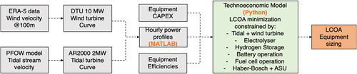
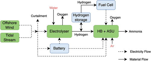
Wind and tidal energy are used to supply power to three components: the electrolyzer to produce hydrogen, a battery, and the air separation unit (ASU) to produce nitrogen in addition to the Haber-Bosch (HB) unit to produce ammonia from nitrogen and hydrogen (Figure 2). To account for variable wind and tidal energy inputs and thus variable hydrogen production in the electrolyzer, hydrogen storage between the electrolyzer and the HB unit is included. A fuel cell is also included to supply back-up electricity to the HB and ASU from stored hydrogen. Battery storage, charged by wind and tidal energy, is used to supply back-up electricity to the electrolyzer, HB and ASU. Electricity can also be curtailed if necessary.

Figure 2. Flow diagram displaying the units involved in ammonia production, electricity flow between them and material inputs and outputs. Internal energy storage units are in blue.

The ammonia plant optimization model minimizes the levelized cost of ammonia, $LCOA$ (USD/t) – Eq.. 1.

(1) $LCOA=\frac{\left(\frac{i{\left(1+i\right)}^{PL}}{{\left(1+i\right)}^{PL}-1}\right)\times CAPEX+OPEX}{F}$(1)

where $F$ is the yearly ammonia production in tons (set to 100,000 tons/year), $i$ is the discount rate of 7% (Salmon, Bañares-Alcántara, and Nayak-Luke 2021) and $PL$ is plant lifetime, assumed to be 30 years.

The total $CAPEX$ (USD) calculation is presented in Eq.. 2, and individual equipment CAPEX values are listed in Table A1.

(2) $CAPEX=\sum {\sigma }_{R}Cos{t}_R+\sum {\sigma }_{C}Cos{t}_C+\sum {\sigma }_{SC}Cos{t}_{SC}+{\sigma }_{FC}Cos{t}_{FC}+Cos{t}_P$(2)

where ${\sigma }_R$ is the installed capacity of the renewable energy source (MW), $Cos{t}_R$ is the cost of renewable power (USD/MW), ${\sigma }_C$ is the installed capacity of the component (MW), $Cos{t}_C$ is the cost of the component (USD/MW), ${\sigma }_{SC}$ is the installed capacity of the storage component (MWh for battery, t for hydrogen), $Cos{t}_{SC}$ is the cost of the storage component (USD/MWh for battery, USD/t for hydrogen), ${\sigma }_{FC}$ is the installed capacity of the fuel cell (MW), $Cos{t}_{FC}$ is the cost of fuel cell (USD/MW), and $Cos{t}_P$ is the cost of offshore platform (USD). Renewable energy sources considered are tidal stream and wind. Components considered are the electrolyzer, HB+ASU, and battery interface (for power sizing). As described in Appendix A, the tidal turbine CAPEX is appropriate for 100 MW of tidal capacity. There is a large uncertainty in the tidal turbine CAPEX, thus an upper and lower bound will be applied in the model. Storage components considered are battery and hydrogen storage. The battery self-discharge is 5% per month (Salmon and Bañares-Alcántara 2021b). The HB ramp up and down limits are 2% per hour and 20% per hour respectively (Fasihi et al. 2021). The minimum load of the HB is 20% of rated capacity (Beerbühl, Fröhling, and Schultmann 2015). The electrolyzer is assumed to ramp up and down instantaneously and is modeled with a constant conversion efficiency of $50kWhk{g}^{-1}$ (Nayak-Luke and Bañares-Alcántara 2020; Salmon and Bañares-Alcántara 2021b). The last 14 days of every year modeled are allocated to maintenance time (Salmon and Bañares-Alcántara 2021b), whereby no ammonia is produced. Hence, an operational year is 8,424 hours (365 days minus 14 days). However, ideally, maintenance could be done during the least productive power periods.

The total $OPEX$ (USD/y) is presented in Eq. 3:

(3) $OPEX=\frac{CF\left(H_{2}O,H_2\right)}{CF\left(N{H}_3,H_2\right)}Cos{t}_{W}F+Cos{t}_{OM}CAPEX$(3)

where $Cos{t}_W$ is the cost of desalinated water (2 USD/t (Salmon and Bañares-Alcántara 2021b)) and $Cos{t}_{OM}$ are the operating and maintenance costs (2% of CAPEX (Salmon and Bañares-Alcántara 2021b)). The conversion factors are $CF\left(H_{2}O,H_2\right)$, water to hydrogen mass ratio, and $CF\left(N{H}_3,H_2\right)$, ammonia to hydrogen mass ratio. From stoichiometry: $CF\left(H_{2}O,H_2\right)=9k{g}_{H_{2}O}/k{g}_{H_2}$ and $CF\left(N{H}_3,H_2\right)=17/3k{g}_{N{H}_3}/k{g}_{H_2}$.

To account for different energy sources and variability of wind, two studies are simulated:

1. Low, baseline, and high wind years for both tidal and wind vs wind only, i.e. 6 scenarios.

2. 30 consecutive years, representing the plant’s lifetime, for both tidal and wind vs wind only, i.e. 2 scenarios.

A sensitivity analysis is performed on the tidal CAPEX value relative to the wind CAPEX value to determine the cutoff CAPEX values at which no tidal and all wind is utilized by the techno-economic model and vice versa.

Tidal stream resource

Tidal stream turbine power

The tidal current flow velocity data from the PFOW model (O’Hara Murray and Campbell 2021; O’Hara Murray and Gallego 2017) is used in this research to determine the power variation of an Atlantis AR2000 tidal turbine in the Pentland Firth (the AR2000 will be utilized in the MeyGen Project (Black and Veatch 2020)). The AR2000 has a rated capacity of 2 MW, a cut-in velocity of <1 m/s, rated velocity of 3.05 m/s and rotor diameter of 20 m (Encarnacion, Johnstone, and Ordonez-Sanchez 2019; Lewis et al. 2021).

The tidal turbine power $P\left(MW\right)$ is determined (as shown in Appendix B) using Eq.. 4:

(4) $P=\frac{1}{2}\rho A{C}_p{u}^3$(4)

where $\rho$ is the density of fluid, $A$ is the swept area of turbine, $C_p$ is the power coefficient and $u$ is the fluid velocity.

The velocities at each location are taken as the average of the middle three sigma layers. This is to account for the location of the turbine in the water. Yang et al (2013). demonstrate that the location of the largest power output of a tidal turbine is at the middle of the water column.

Tidal stream turbine location and layout

The ideal tidal turbine location is where the tidal stream currents are reliably and consistently fast. This results in a large power output from the turbines over a period of time, requiring fewer turbines to produce a fixed amount of ammonia, which will enable a lower LCOA. Thus, a region in the Pentland Firth with high annual energy production from tidal turbines is chosen for analysis.

Due to local tidal current velocity variation, each tidal turbine will have a different annual energy production capacity.

To determine which tidal turbine power profiles are used as an input to the technoeconomic model, the locations (nodes in the PFOW model) with the largest annual energy production in the region considered are selected, which constrains the layout of tidal turbines. The average power profiles from 100 MW (i.e. 50 locations or nodes) of tidal power capacity were input to the technoeconomic model (Figure 1). The calculated total tidal power capacity output by the technoeconomic model, may be more or less than 100 MW. This is justified since only a small region of the Pentland Firth is exploited for tidal stream power in this paper. Moreover, each node (and thus power profile) could potentially represent more than one turbine, so a capacity output by the technoeconomic model of more than 100 MW is justified. If the capacity output by the technoeconomic model is less than 100 MW, this would be a conservative approximation as fewer, better power profiles (and thus a lower tidal capacity) could represent the required tidal stream power input. The LCOA could be lowered (by a couple percentage points) if the required and calculated tidal turbine power capacities in the ammonia model (Figure 1) are matched. However, using a fixed number of tidal turbine power profiles is a justified engineering approximation for this paper.

Wind resource

Wind turbine power

The wind profile is from ECMWF (European Center for Medium-Range Weather Forecasts) Reanalysis v5 (ERA5) (Hersbach et al. 2022). ERA5 data is reported every hour since 1979 and has a high resolution of 0.25° for latitude and longitude. The north and east velocity components are converted to the resultant velocity for 1991–2020. The reference height, $h_{ref}$, at which the velocities, $u_{ref}$, are reported at in ERA5 is $100m$. In Eq.. 5, the Hellmann exponent, $\alpha$, is about 0.1 for wind turbines above the ocean (Abolude and Zhou 2019; Liu et al. 2017) which allows the wind velocities, $u$, at $h=119m$ (the hub height) to be calculated.

(5) $u=u_{ref}{\left(\frac{h}{h_{ref}}\right)}^{\alpha }$(5)

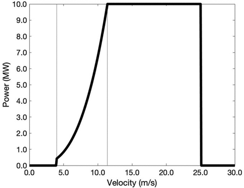
The power curve used is that of the DTU 10 MW wind turbine (Bak et al. 2013) – the cut-in, rated and cutout wind speeds are 4, 11.4, and 25 m/s respectively, the blade diameter is 178.3 m and the hub height is 119 m. Several recent, relevant papers utilizing offshore wind also use the DTU 10 MW turbine including Baldi et al (2022); Martinez and Iglesias (2022); and Wang et al (2020). The wind turbine power is determined using Eq. 4(4) $P=\frac{1}{2}\rho A{C}_p{u}^3$(4) (as shown in Appendix B).

Wind turbine location and layout

The wind location is constrained to the same region of the Pentland Firth with high tidal turbine annual energy production. The wind turbine layout is less constrained compared to the tidal stream turbine layout (in terms of wake recovery distance (Vennell et al. 2015)). Thus, the specific layout of wind turbines will not be considered but rather the maximum limit on wind power in an area will be factored in. The maximum wind turbine power density that avoids hindrance due to wake effects is 5 MWkm⁻² (Ruiz et al. 2019).

Results and discussion

Tidal stream energy in the Pentland Firth

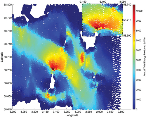
A heat map of the annual energy produced from an isolated, 2 MW tidal turbine within the Pentland Firth is shown in Figure 3. A smaller region within the Pentland Firth with the highest annual energy production is focused upon in the inset of Figure 3. The highest capacity factor in this smaller region is 0.631 with 10,634 MWh of energy produced per year.

Figure 3. Heat map of the annual energy produced from an AR2000 2 MW turbine in the Pentland Firth. The longitude range is (−3.300)-(−2.800) and the latitude range is 58.640–58.800. For the inset, the longitude range is (−3.150)-(−3.050) and the latitude range is 58.690–58.740.

Wind energy in the Pentland Firth

Wind velocities are determined at [−3.24, 58.65], as this is the closest location to the inset of Figure 3. At this wind location, the annual capacity factor is relatively high but variable over 1991–2020 (Figure 4). For Study 1 of the technoeconomic analysis, 2010 is the low wind year (capacity factor 0.488), 2020 is the baseline wind year (capacity factor 0.536) and 2015 is the high wind year (capacity factor 0.589).

Figure 4. Annual capacity factor of a 10 MW DTU offshore wind turbine at [−3.24, 58.65] over the years 1991–2020.

Study 1: low, baseline, and high wind years

Using a basis of 100,000 tons NH₃ produced per year, the model is run for 2010 (low wind year), 2020 (baseline wind year) and 2015 (high wind year).

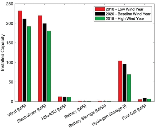
In the wind-only case and compared to a baseline wind year, on a low wind year 10% more wind capacity is required, and on a high wind year 9% less wind capacity is required (Figure 5). This is expected as more wind capacity is necessary to produce 100,000 tons/y of NH₃ on a low wind year and vice versa.

Figure 5. Wind only - comparison of equipment capacities for wind years 2010, 2020 and 2015 (Study 1). The ammonia production is fixed at 100,000 tons/year.

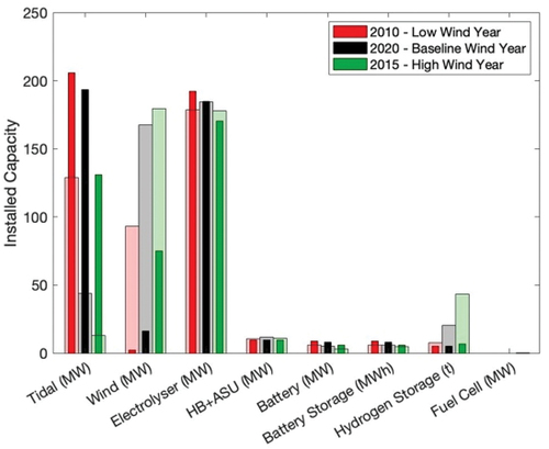
In the wind+tidal case and compared to a baseline wind year, on a low wind year, 86% less wind and 6% more tidal capacity are required, and on a high wind year, 362% more wind and 32% less tidal capacity are required (Figure 6). This makes sense as wind capacity is favored over tidal capacity in a high wind year and vice versa.

Figure 6. Wind+tidal - comparison of equipment capacities for wind years 2010, 2020 and 2015 (Study 1). The ammonia production is fixed at 100,000 tons/year. The wider bars represent the higher value of tidal turbine CAPEX.

The LCOA is 18%, 12%, and 5% lower when tidal capacity is added to wind capacity in 2010, 2020 and 2015 respectively (Figure 7), quantifying the benefit of utilizing tidal stream energy for ammonia production.

Figure 7. Comparison of LCOA for wind+tidal vs. wind only for wind years 2010, 2020 and 2015 (Study 1). The ammonia production is fixed at 100,000 tons/year. The historical brown ammonia price range is 100–600 USD/t (IRENA 2022). The wider bars represent the higher value of tidal turbine CAPEX.

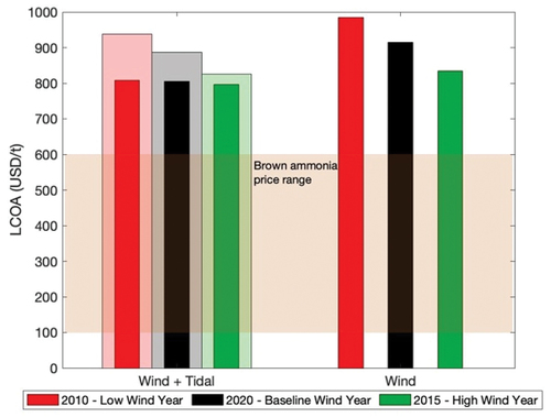
When the higher value of the tidal turbine CAPEX is used, significantly more wind and less tidal is utilized, which is expected, as the ammonia model operates to minimize the LCOA. The LCOA is still lower when tidal capacity is added to wind capacity, but by a smaller margin (by 5%, 3%, and 1% in 2010, 2020 and 2015 respectively).

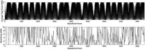
Comparing the wind and tidal case (Figure 6) to the wind-only case (Figure 5), significantly less fuel cell capacity and hydrogen storage are required for the former. Figure 8 helps to explain this behavior: tidal stream power displays a different, more consistent power profile compared to wind power, demonstrating the practical benefit of utilizing tidal stream energy.

Figure 8. Power profile for an average tidal turbine and wind turbine over the 2020 operational year.

In each case (Figure 7), the LCOA is above the historical (2000–2020) brown ammonia price range (100–600 USD/t (IRENA 2022)). Current brown ammonia prices are discussed in section 3.4.

Study 2: consecutive wind years

The results for three separate wind years are useful to show how wind variability must be incorporated to plant design, but it is unrealistic to run the plant with a different number of tidal turbines and wind turbines each year. Running 30 years of consecutive wind and tidal data gives a robust plant design and a single installed capacity value for each piece of equipment. Using the same basis of 100,000 tons NH₃ per year, the model is run for 30 consecutive years, 1991–2020.

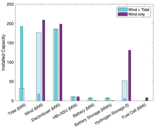
In the wind-only case, 209 MW of wind is required (Figure 9). In the wind+tidal case, 17 MW of wind and 192 MW of tidal are required. When the higher value of the tidal turbine CAPEX is used, in the wind+tidal case, 176 MW of wind and 32 MW of tidal are required. Similar to Study 1, when the higher value of the tidal turbine CAPEX is used, significantly more wind and less tidal is utilized, which makes sense. Moreover, if adding tidal capacity to wind capacity were not economically beneficial, the technoeconomic model would not utilize tidal capacity. Since the tidal capacity utilized is large relative to the wind capacity utilized (in the wind+tidal case with the lower tidal CAPEX case), utilizing tidal can be remarkably beneficial.

Figure 9. Comparison of equipment capacities for wind+tidal vs. wind only for consecutive wind years 1991–2020 (Study 2). The ammonia production is fixed at 100,000 tons/year. The wider bars represent the higher value of tidal turbine CAPEX.

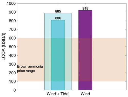
The LCOA for green ammonia utilizing wind+tidal (806 USD/t or 885 USD/t when the higher value of the tidal turbine CAPEX is used), and wind only (918 USD/t) is not competitive with the historical (2000–2020) brown ammonia price range (Figure 10). However, current gray ammonia prices are > 1,000 USD/t due to natural gas shortages (IRENA 2022). Moreover, according to IRENA and AEA, the general LCOA for green ammonia is 720–1,400 USD per ton today (and is predicted to drop to 310–610 USD per ton in 2050) (IRENA 2022). Thus, the LCOA for both wind+tidal and wind only in this paper are economically attractive compared to green and gray ammonia today. This could enhance the capacity of the UK to produce ammonia locally, which is important in the context of energy security.

Figure 10. Comparison of LCOA for wind+tidal vs. wind only for consecutive wind years 1991–2020 (Study 2). The ammonia production is fixed at 100,000 tons/year. The historical brown ammonia price range is 100–600 USD/t (IRENA 2022). The wider bars represent the higher tidal turbine CAPEX.

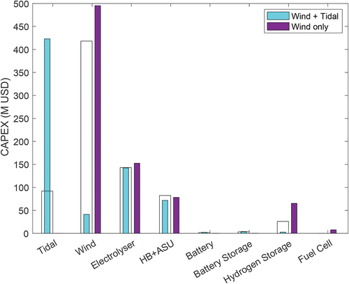
Similar to Study 1, the LCOA is lower (by 12% or 4% when the lower/higher value of the tidal turbine CAPEX is used) when tidal capacity is added to wind capacity. This is primarily due to the significantly reduced storage requirements: the wind+tidal case requires no fuel cell capacity and up to 96% less hydrogen storage (corresponding to a 63 M USD CAPEX reduction – Figure 11) compared to the wind-only case. However, the wind+tidal case requires up to 7.3 MWh more battery storage (minimal CAPEX increase of around 3 M USD) compared to the wind-only case, due to the (predictable) short-term tidal power variation. The total renewables CAPEX is 464–510 M USD for the wind+tidal case and 495 M USD for the wind-only case. The electrolyzer requires the largest capacity in the ammonia plant and a 6–7% lower electrolyzer capacity is required for the wind+tidal case compared to the wind-only case (corresponding to a 9–10 M USD lower CAPEX).

Figure 11. Comparison of Equipment CAPEX for wind+tidal vs. wind only for consecutive wind years 1991–2020 (Study 2). The ammonia production is fixed at 100,000 tons/year. The wider bars represent the higher value of tidal turbine CAPEX.

Since the fuel cell is not utilized in the wind+tidal case, the HB and ASU can operate successfully from wind and tidal energy with battery back-up. Moreover, in the wind-only case, all three internal energy storage assets (battery storage, hydrogen storage and fuel cell capacity) are needed.

In both studies, the curtailed energy is < 3% which is relatively low.

Tidal and wind turbine arrangement

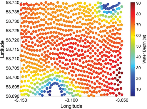
Figure C1 (in Appendix C) shows the layout of the tidal turbines which have a downstream spacing of approximately 200 m (10D). As described in the introduction, streamwise spacing of turbines should be between 10-20D to allow for wake recovery (Almoghayer et al. 2022; Stallard et al. 2013). Thus, the spacing of tidal turbines is on the borderline of the acceptable limit.

ERA5 wind velocity data has a resolution of 0.25° by 0.25° (Hersbach et al. 2022) which, at a latitude of 58.65°, is 404 km². As previously mentioned, the maximum wind turbine power density that avoids hindrance due to wake effects is 5 MW km⁻² (Ruiz et al. 2019). Thus, 2020 MW is the maximum capacity of wind at [−3.24, 58.65]. In both studies, the wind capacity required is an order of magnitude lower than 2020 MW.

Comparison of offshore and onshore cost

The results in this paper are valid for offshore ammonia production. The offshore platform cost for ammonia production is substantial (see Table A1). Onshore production of ammonia may be more appropriate since the tidal turbines that are utilized are close to shore (~10 km). The cost of a HVDC offshore cable is 1.1 M GBP/km (Nieradzinska et al. 2016) for a maximum of 1.2 GW of power. Thus, around 11 M GBP is required for an offshore cable, which is an order of magnitude lower than the cost of an offshore ammonia platform (120 M USD (Wang, Daoutidis, and Zhang 2021)).

Thus, while offshore production is likely to be more expensive than onshore production, in general land limitations and restrictions may motivate offshore ammonia production, particularly for places such as the UK which have low land availability but good offshore energy resources (Salmon and Bañares-Alcántara 2022).

Tidal CAPEX sensitivity

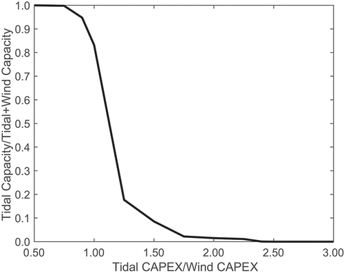
The tidal turbine CAPEX has a large uncertainty, so an upper and lower bound was incorporated into the analysis, corresponding to 1.22 and 0.93 times the wind CAPEX. Moreover, in Section 1.1., it is acknowledged that in the UK today, tidal stream energy has an LCOE three times larger than offshore wind energy (Coles et al. 2021). To see the extent to which the techno-economic model utilizes tidal capacity over wind capacity, the tidal CAPEX is varied from 0.5 to 3 times the wind CAPEX (Figure 12 - using the baseline wind year, 2020). When the tidal CAPEX is less than around 0.75 times the wind CAPEX, the techno-economic model utilizes all tidal capacity and no wind capacity. However, when the tidal CAPEX is more than around 2.4 times the wind CAPEX, the techno-economic model utilizes all wind capacity and no tidal capacity. These cutoff values will likely vary with location-dependent wind and tidal power profiles, the time frame (e.g. 1 year or 30 years), as well as the relative energy storage equipment CAPEX costs. Interestingly, when the tidal and wind CAPEX values are equal, around 83% of the renewable capacity is tidal capacity. Thus, tidal stream power is a better renewable resource than offshore wind power for this green ammonia production scenario.

Figure 12. Sensitivity of tidal CAPEX relative to wind CAPEX and the impact on the fraction of tidal capacity out of the total renewable capacity (tidal and wind) that the techno-economic model utilizes. A single baseline wind year, 2020, is used for the wind power profile.

Limitations of the research

In order to model the green ammonia plant, powered by wind and tidal stream energy, practical modeling decisions were made. There are five modeling decisions which could be further improved.

Firstly, the power coefficient of each tidal turbine and wind turbine is assumed constant, in line with Lewis et al (2021), although the power coefficient may vary with velocity, turbulence and blade design (Mason-Jones et al. 2012).

Secondly, the average of the middle three sigma layers is used to find the tidal stream velocity values. This may not be representative of the actual velocity profile that enters the turbine since the turbine may not be located exactly in the middle of the water column at all locations considered. To account for this, O’Hara Murray and Gallego (2017) include a factor in the velocity terms to account for the percentage of the area of the turbine (perpendicular to the flow) in each sigma layer. This may be a more accurate way to represent the velocity profile entering the turbine.

Thirdly, the tidal turbine CAPEX was not specific to an AR2000, due to lack of public information. More accurate tidal stream turbine CAPEX values should be used in future work, for example, using the Metric Space criterion designed by Garcia‐Sanz (2020) at the ARPA‐E ATLANTIS program (U.S. Department of Energy).

In the wind-only case there are consecutive hours when there is no wind power. However, the Haber-Bosch reactor still operates at 20% capacity, requiring significant hydrogen storage and fuel cell capacity. It could be economically beneficial to shut down the plant when there is an extended period of low wind power input. To achieve this, instead of having maintenance time at the last 14 days of the year, the maintenance time could be optimized to a particularly low wind power period.

Finally, to account for wake recovery, the tidal turbines are approximately spaced within the suggested limit (10-20D (Almoghayer et al. 2022; Stallard et al. 2013)). To more accurately account for wake effects and turbine interaction, 3D hydrodynamic modeling, such as O’Hara Murray and Gallego (2017), is likely required. Blockage correction factors could also be applied, as detailed by Zilic de Arcos et al (2020). In a constrained flow, the fluid flow is affected by neighboring boundaries (e.g. tidal turbines, foundations or the sea floor) and this is known as blockage. When the fraction of the channel cross-sectional area occupied by the turbine swept area is more than 10%, blockage corrections are required (Djama Dirieh et al. 2022; Thiébot et al. 2020).

Conclusions

The objective of this paper was to determine if tidal stream energy is a useful energy resource (technically and economically) for offshore green ammonia production. The case study on the Pentland Firth demonstrated that producing green ammonia from tidal and wind energy resources is technically feasible and economically attractive compared to conventional green ammonia from solar and wind onshore (in 2020). For both wind+tidal vs. wind only, two studies are simulated; firstly, using separate low, baseline, and high wind years to show the impact of variable wind years on LCOA and secondly, using 30 consecutive wind years – representing the plant’s lifetime.

For the 30-year study, the LCOA for green ammonia utilizing wind+tidal (806 USD/t), and wind only (918 USD/t) is lower than recent gray ammonia prices (>1,000 USD/t given natural gas shortages (IRENA 2022)) but higher than the historical brown ammonia price (100–600 USD/t (IRENA 2022)). Adding tidal stream capacity to wind capacity decreases the hydrogen storage requirement by 96% and eliminates the fuel cell requirement and thus reduces the LCOA (by 12%). In the first study, for low, baseline, and high wind years, the LCOA is 5–18% lower when tidal capacity is added to wind capacity. When the higher tidal turbine CAPEX is used, the LCOA is also lower, but by a smaller margin (1–5%). Thus, utilizing tidal stream power is economically beneficial in both cases.

A sensitivity analysis was performed on the tidal CAPEX – the tidal CAPEX was varied from 0.5 to 3 times the wind CAPEX to see the extent to which the techno-economic model utilizes tidal capacity over wind capacity. Using the baseline wind year, 2020, it is shown that when the tidal and wind CAPEX values are equal, tidal capacity dominates (83%) the total renewable capacity, demonstrating the adequacy of tidal power as an energy source for green ammonia production.

Similar to other technoeconomic analyses of green ammonia production, for example, Cesaro et al (2021), it would be beneficial to predict the LCOA range in the future for green ammonia production from tidal stream power, including upper and lower bounds on model inputs such as electrolyzer CAPEX.

This study did not include the cost benefits of higher predictability (i.e. less buffer storage) in the actual operation of the ammonia plant from tidal stream power, nor tidal-only green ammonia production analysis in the Pentland Firth and in other tidal hotspots; these matters should be explored in future work.

Given the global transition to green ammonia from conventional high-carbon ammonia, it is valuable to identify all suitable sources of renewable energy. Tidal stream energy is a novel and ideal energy source for offshore green ammonia production given its high resource availability and predictability.

Glossary

Acronyms	=
LCOA	=	Levelized cost of ammonia
LCOE	=	Levelized cost of energy
PFOW	=	Pentland Firth and Orkney Waters
FVCOM	=	Finite Volume Community Ocean Model
HB	=	Haber-Bosch
ASU	=	Air separation unit
ERA5	=	ECMWF (European Centre for Medium-Range Weather Forecasts) Reanalysis v5
OPEX	=	Operating cost
CAPEX	=	Capital cost
MILP	=	Mixed-integer linear program
Symbols	=
$F$	=	Yearly ammonia production (tons/year)
$i$	=	Discount rate (%)
$PL$	=	Plant lifetime (years)
${\sigma }_R$	=	Installed capacity of the renewable energy source (MW)
$Cos{t}_R$	=	Cost of renewable power (USD/MW)
${\sigma }_C$	=	Installed capacity of the component (MW)
$Cos{t}_C$	=	Cost of the component (USD/MW)
${\sigma }_{SC}$	=	Installed capacity of the storage component (MWh for battery, t for hydrogen)
$Cos{t}_{SC}$	=	Cost of the storage component (USD/MWh for battery, USD/t for hydrogen)
${\sigma }_{FC}$	=	Installed capacity of the fuel cell (MW)
$Cos{t}_{FC}$	=	Cost of fuel cell (USD/MW)
$Cos{t}_P$	=	Cost of offshore platform (USD)
$CF$	=	Conversion factor
$Cos{t}_W$	=	Cost of desalinated water (USD/t)
$Cos{t}_{OM}$	=	Operating and maintenance costs (% of CAPEX)
$P$	=	Power (MW)
$\rho$	=	Density of fluid (kg/m3)
$A$	=	Swept area of turbine (m2)
$C_p$	=	Power coefficient
$u$	=	Fluid velocity (m/s)
$u_{ref}$	=	Reference velocity (m/s)
$h_{ref}$	=	Reference height (m)
$h$	=	Wind turbine hub height (m)
$\alpha$	=	Hellmann exponent
$C$	=	Capital cost of offshore platform (USD)
$b$	=	Water depth (m)
$D$	=	Plant capacity (t/day)
$P_r$	=	Maximum power (MW)
$u_r$	=	Rated velocity (m/s)
$u_s$	=	Cut-in velocity (m/s)
$u_o$	=	Cut-out velocity (m/s)
$r$	=	Radius of turbine (m)
$u_{north},u_{east}$	=	Velocity in the northern and eastern directions (m/s)

Acknowledgements

The use of MATLAB and its toolboxes was under an academic license. The use of Gurobi was under a free academic license.

Disclosure statement

No potential conflict of interest was reported by the author(s).

Data availability statement

The data that support the findings of this study are openly available from Copernicus Climate Change Service (C3S) Climate Data Store (CDS) at https://cds.climate.copernicus.eu/cdsapp#!/dataset/reanalysis-era5-single-levels and Marine Scotland at https://data.marine.gov.scot/dataset/pentland-firth-and-orkney-waters-climatology-102.

Additional information

Funding

This work was supported by a studentship from UKRI for the first author [project reference: 2594549] and a Rhodes Trust scholarship for the second author.

Notes on contributors

Honora Driscoll

Honora Driscoll obtained her MEng degree in Chemical Engineering from University College London (UCL) in 2021 and is in her second year as a PhD student at the University of Oxford. She has held internships at the Los Alamos and Lawrence Berkeley National Laboratories in the USA. Her research is focused on the use of tidal and wind energy for the offshore production of green ammonia.

Nicholas Salmon

Nicholas Salmon obtained his Master’s degree in Chemical Engineering from the University of Queensland in 2017, and is now pursuing a PhD at the University of Oxford. His research focusses on understanding how green ammonia can be used to decarbonise global energy systems, with particular focus on transporting it from regions with high renewable energy potential to regions without that potential.

Rene Bañares-Alcántara

René Bañares-Alcántara is a Reader in Engineering Science at the University of Oxford and Senior Tutor for Engineering at New College. He holds a BEng from UNAM (Mexico), and an MSc and PhD from Carnegie Mellon University (Pittsburgh, USA), all of them in Chemical Engineering. His research interests are around Process Systems Engineering and since 2014 he has focused on long-term (chemical) storage of renewable energy and the production, distribution, and use of ‘green’ ammonia (https://eng.ox.ac.uk/green-ammonia/). He has (co-)authored about 70 journal papers and around 100 other refereed publications of various kinds.

Appendix A.

Equipment CAPEX details

Table A1. CAPEX values for equipment used in the technoeconomic Python model for green ammonia production. 2020 USD is used. (*) denotes that the CAPEX value is justified in Appendix A.

Equipment	CAPEX	Reference
HB+ASU CAPEX	7,444 USD kW − 1	(Salmon and Bañares-Alcántara 2021b)
Hydrogen storage	500 USD kg − 1	(Nayak-Luke and Bañares-Alcántara 2020)
Fuel cell	960 USD kW − 1	(Nayak-Luke and Bañares-Alcántara 2020)
Electrolyser	770 USD kW − 1	(IRENA 2020)
Battery interface (Lithium Ion)	271 USD kW − 1	(Cesaro et al. 2021)
Battery storage (Lithium Ion)	500 USD kW −1 h − 1	(Salmon and Bañares-Alcántara 2021b)
Offshore platform*	120 M USD	(Wang, Daoutidis, and Zhang 2021)
Tidal stream turbine* (Generic 2 MW)	2,200 (lower)2,900 (upper)USD kW − 1 2,900 (upper) USD kW^−1	(Goss, Coles, and Piggott 2021)
Wind turbine* (Generic Offshore)	2,372 USD kW − 1	(IRENA 2022)

Tidal turbine CAPEX

The tidal turbine CAPEX estimate is from Goss et al. (2021) and is dependent on the number of turbines in the array and the capacity of each turbine. For 50, 2 MW turbines, the average typical and conservative CAPEX/MW is 2.2 and 2.9 M USD/MW, respectively. It is acknowledged that current tidal CAPEX values are higher than these values due to the current low deployment of tidal stream in the UK (on the order of 10 MW) (Coles et al. 2021). However, for 100 MW, the tidal CAPEX is expected to be considerably less than current values (due to the high learning rate of 26% below 100 MW (Coles et al. 2021)). It is assumed that no export cables (to shore) are needed, since the ammonia plant modeled is offshore. Thus cabling, representing ~ 10% of the total CAPEX, is not included (Black and Veatch 2020) (this value varies from 9-14% (Coles et al. 2021; Goss, Coles and Piggott 2021). Cables between the turbines and the ammonia plant will still be needed. However, the length and number of cables depends on plant design.

Wind turbine CAPEX

Fixed-bottom wind turbines are appropriate for water depths <60 m (Wang, Daoutidis and Zhang 2021). There are locations in the Pentland Firth with water depths of <60 m (Figure C2–Appendix C). Thus, the wind turbine CAPEX is estimated from the worldwide average installed cost of fixed-bottom offshore wind turbines [IRENA 2022] (cabling, representing ~ 17% of the total CAPEX is not included).

Offshore platform CAPEX

The capital cost of an offshore platform for ammonia production is difficult to estimate, due to its novelty. Wang et al. (2021) use a cost correlation, altered from newbuild, jackup platform offshore oil rigs in Kaiser et al. (2013) (in the region considered, the water depths are <168 m, thus fixed jackup platforms are appropriate).

The capital cost ($C$ in USD) varies with water depth ($b$ in meters) and plant capacity ($D$ in t/day) as shown in Equation A1(A1) $C=\left(1+\frac{0.25D}{3000}\right)\times \left(7.37\times {10}^7+8.61\times {10}^3{b}^2\right)$(A1) .

(A1) $C=\left(1+\frac{0.25D}{3000}\right)\times \left(7.37\times {10}^7+8.61\times {10}^3{b}^2\right)$(A1)

$D=285t/day$ for 100,000 ton NH₃/year (1 operational year is 8,424 hours). $b=\text{~}70m$ in the region of the Pentland Firth considered. Thus, $C=120MUSD$.

Appendix B.

Power calculation for Wind and Tidal turbines

Tidal Turbine power calculation

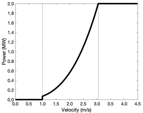
The power curve for an AR2000 2 MW tidal turbine (Figure B1) is determined from the following constraints:

If $u_s\le u\le u_r$, $P=\frac{1}{2}\rho A{C}_p{u}^3$

If $u<u_s$, $P=0W$

If $u>u_r$, $P=P_r$

Where $P_r$ is maximum power, $u_r$ is rated velocity and $u_s$ is cut-in velocity. For the AR2000 2 MW tidal turbine: $u_r=3.05m/s$ and $u_s=1m/s$ (Lewis et al. 2021). The parameters values are: $p=1,027kg/m^3$ (Lewis et al. 2021) and $A=\pi r^2=\pi {\left(\frac{20}{2}m\right)}^2$ (radius, $r$, of the turbine is 10 m (Encarnacion, Johnstone and Ordonez-Sanchez 2019)) and $C_p=0.437$ as calculated below:

(A2) $C_p=\frac{P_r}{\frac{1}{2}\rho A{u_r}^3}=\frac{2MW}{\frac{1}{2}\times 1,027\frac{kg}{m^3}\times \left(\frac{1}{4}\pi \times {\left(20\mathrm{m}\right)}^2\right)\times {\left(3.05\frac{m}{s}\right)}^3\times {10}^{-6}\frac{MW}{W}}=0.437\left(3dp\right)$(A2)

The power coefficient, $C_p$, is assumed to be the same from the cut-in velocity to the rated velocity. The cut-out velocity is not required for tidal stream turbines but is required for wind turbines since the range of tidal current speeds is not as large as wind speeds (Liu et al. 2015).

Figure B1. Power curve for an AR2000 2MW tidal turbine.

Wind Turbine power calculation

The power curve for a DTU 10 MW wind turbine (Figure B2) is determined according to the following constraints:

If $u_s\le u\le u_r$, $P=\frac{1}{2}\rho A{C}_p{u}^3$

If $u<u_s$, $P=0W$

If $u_r<u<u_o$, $P=P_r$

If $u\ge u_o$, $P=0W$

where $u_o$ is cut-out velocity. For the DTU 10 MW wind turbine: $u_r=11.4m/s$, $u_s=4\hspace{0.17em}m/s$ and $u_o=25\mathrm{m}/\mathrm{s}$ (Bak et al. 2013). The parameters values are: $\rho =1.225\frac{kg}{m^3}$ (the density of air is assumed to not vary with time which is typical in wind power literature (Ulazia et al. 2019)), $A=\pi r^2=\pi {\left(\frac{178.3}{2}m\right)}^2$ (radius, $r$, of the turbine is $\frac{178.3}{2}m$ (Bak et al. 2013)) and $C_p=0.441$ as calculated below:

(A3) $C_p=\frac{P_r}{\frac{1}{2}\rho A{u_r}^3}=\frac{10MW}{\frac{1}{2}\times 1.225\frac{kg}{m^3}\times \left(\frac{1}{4}\pi \times {\left(178.3\mathrm{m}\right)}^2\right)\times {\left(11.4\frac{m}{s}\right)}^3\times {10}^{-6}\frac{MW}{W}}=0.441\left(3dp\right)$(A3)

For both the tidal turbine and the wind turbine, the velocity is determined using $u=\sqrt{{u_{north}}^2+{u_{east}}^2}$. $u_{north}$ and $u_{east}$ are the velocity values in the northern and eastern directions, respectively.

The power coefficient, $C_p$, is assumed to be the same from the cut-in velocity to the rated velocity.

Figure B2. Power curve for a DTU 10 MW wind turbine.

Appendix C.

Layout of Tidal Turbines and Water Depth in Pentland Firth

Figure C1. Tidal turbine layout for the wind+tidal scenarios of Study 1 and Study 2.

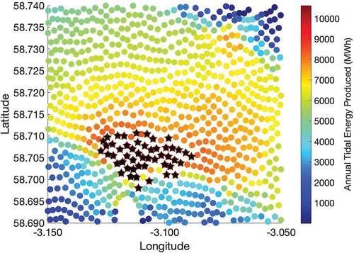
Figure C2. Water depth in a region of the Pentland Firth (depth data from the PFOW model (O’Hara Murray and Gallego 2017); (O’Hara Murray and Campbell 2021).

References

- Abolude, A., and W. Zhou. 2019. A comparative computational fluid dynamic study on the effects of terrain type on hub-height wind aerodynamic properties. Energies 12 (1):83. doi:10.3390/en12010083.
- Alex, A., R. Petrone, B. Tala-Ighil, D. Bozalakov, L. Vandevelde, and H. Gualous. 2022. Optimal techno-enviro-economic analysis of a hybrid grid connected tidal-wind-hydrogen energy system. International Journal of Hydrogen Energy 47 (86):36448–64. doi:10.1016/j.ijhydene.2022.08.214.
- Almoghayer, M. A. and D. K. Woolf. 2019. An assessment of efficient tidal stream energy extraction using 3D numerical modelling techniques. In: Proceedings of the 13th EWTEC, 1-6 September, Naples, Italy, 1–10.
- Almoghayer, M. A., D. K. Woolf, S. Kerr, and G. Davies. 2022. Integration of tidal energy into an island energy system - a case study of Orkney islands. Energy 242:122547. doi:10.1016/j.energy.2021.122547.
- Bak, C. 2013. The DTU 10-MW reference wind turbine. In: Danish wind power research 2013, DTU Risø Campus, Denmark.
- Baldi, F., A. Coraddu, M. Kalikatzarakis, D. Jeleňová, M. Collu, J. Race, and F. Maréchal. 2022. Optimisation-based system designs for deep offshore wind farms including power to gas technologies. Applied Energy 310:118540. doi:10.1016/j.apenergy.2022.118540.
- Beerbühl, S. S., M. Fröhling, and F. Schultmann. 2015. Combined scheduling and capacity planning of electricity-based ammonia production to integrate renewable energies. European Journal of Operational Research 241 (3):851–62. doi:10.1016/j.ejor.2014.08.039.
- Black & Veatch. 2020. “Lessons learnt from MeyGen Phase 1A final summary report,” Surrey, UK.
- Blanco, H., W. Nijs, J. Ruf, and A. Faaij. 2018. Potential of power-to-methane in the EU energy transition to a low carbon system using cost optimization. Applied Energy 232:323–40. doi:10.1016/j.apenergy.2018.08.027.
- Bryden, I. G., T. Grinsted, and G. T. Melville. 2004. Assessing the potential of a simple tidal channel to deliver useful energy. Applied Ocean Research 26 (5):198–204.
- Cesaro, Z., M. Ives, R. Nayak-Luke, M. Mason, and R. Bañares-Alcántara. 2021. Ammonia to power: Forecasting the levelized cost of electricity from green ammonia in large-scale power plants. Applied Energy 282:116009. doi:10.1016/j.apenergy.2020.116009.
- Coles, D., A. Angeloudis, D. Greaves, G. Hastie, M. Lewis, L. Mackie, J. McNaughton, J. Miles, S. Neill, M. Piggott, et al. 2021. A review of the UK and British channel Islands practical tidal stream energy resource. Proceedings of the Royal Society A. 477(2255):20210469. doi:10.1098/rspa.2021.0469.
- Crivellari, A., and V. Cozzani. 2020. Offshore renewable energy exploitation strategies in remote areas by power-to-gas and power-to- liquid conversion. International Journal of Hydrogen Energy 45 (4):2936–53. doi:10.1016/j.ijhydene.2019.11.215.
- Djama Dirieh, N., J. Thiébot, S. Guillou, and N. Guillou. 2022. Blockage corrections for tidal turbines—application to an array of turbines in the Alderney race. Energies 15 (10):3475. doi:10.3390/en15103475.
- Encarnacion, J. I., C. Johnstone, and S. Ordonez-Sanchez. 2019. Design of a horizontal axis tidal turbine for less energetic current velocity profiles. Journal of Marine Science and Engineering 7 (7):197. doi:10.3390/jmse7070197.
- Fasihi, M., R. Weiss, J. Savolainen, and C. Breyer. 2021. Global potential of green ammonia based on hybrid PV-wind power plants. Applied Energy 294:116170.
- Garcia‐Sanz, M. 2020. A metric space with LCOE isolines for research guidance in wind and hydrokinetic energy systems. Wind Energy 23 (2):291–311.
- Goss, Z., D. Coles, and M. Piggott. 2021. Economic analysis of tidal stream turbine arrays: A review. 1–29.
- Goward Brown, A. J., S. P. Neill, and M. J. Lewis. 2017. Tidal energy extraction in three-dimensional ocean models. Renew Energy 114:244–57. doi:10.1016/j.renene.2017.04.032.
- Hersbach, H., Bell, B., Berrisford, P., Biavati, G., Horányi, A., Muñoz Sabater, J., Nicolas, J., Peubey, C., Radu, R., Rozum, I., et al. 2022. ERA5 hourly data on single levels from 1979 to present,” Copernicus climate change service (C3S) Climate data store (CDS). Online. Accessed: 10-Mar-2022. doi:10.24381/cds.adbb2d47.
- Ikäheimo, J., J. Kiviluoma, R. Weiss, and H. Holttinen. 2018. Power-to-ammonia in future North European 100 % renewable power and heat system. International Journal of Hydrogen Energy 43 (36):17295–308. doi:10.1016/j.ijhydene.2018.06.121.
- IRENA and AEA. 2022. “Innovation outlook: Renewable ammonia,” International renewable energy agency, Abu Dhabi. Brooklyn: Ammonia Energy Association.
- IRENA (International Renewable Energy Agency). Global renewables outlook: energy transformation 2050. 2020. Abu Dhabi, United Arab Emirates.
- IRENA (International Renewable Energy Agency), “Renewable power generation costs in 2021,” Abu Dhabi, United Arab Emirates, 2022.
- Kaiser, M. J., B. Snyder, and A. G. Pulsipher. 2013. Offshore Drilling Industry and Rig Construction Market in the Gulf of Mexico. BOEM 2013-0112. New Orleans, LA: U.S. Dept. of the Interior, Bureau of Ocean Energy Management, Gulf of Mexico OCS Region.
- Lewis, M., R. O’Hara Murray, S. Fredriksson, J. Maskell, A. de Fockert, S. P. Neill, and P. E. Robins. 2021. A standardised tidal-stream power curve, optimised for the global resource. Renewable Energy 170:1308–23. doi:10.1016/j.renene.2021.02.032.
- Liu, Y., D. Chen, Q. Yi, and S. Li. 2017. Wind profiles and wave spectra for potential wind farms in South China Sea. Part I: Wind speed profile model. Energies 10 (1):125. doi:10.3390/en10010125.
- Liu, M., W. Li, R. Billinton, C. Wang, and J. Yu. 2015. Probabilistic modeling of tidal power generation. In: 2015 IEEE Power & Energy Society General Meeting, Denver, Colorado. 3–7.
- Martinez, A., and G. Iglesias. 2022. Mapping of the levelised cost of energy for floating offshore wind in the European Atlantic. Renewable and Sustainable Energy Reviews 154:111889. doi:10.1016/j.rser.2021.111889.
- Mason-Jones, A., O'Doherty, D.M., Morris, C.E., O'Doherty, T., Byrne, C.B., Prickett, P.W., Grosvenor, R.I., Owen, I., Tedds, S., and Poole, R.J. 2012. Non-dimensional scaling of tidal stream turbines. Energy 44 (1):820–29. doi:10.1016/j.energy.2012.05.010.
- McKenna, R., M. D’Andrea, and M. G. González. 2021. Analysing long-term opportunities for offshore energy system integration in the Danish North Sea. Advances in Applied Energy 4:100067. doi:10.1016/j.adapen.2021.100067.
- “MEYGEN,” SIMEC Atlantis Energy, 2021. [Accessed 2021 Nov 14]. [Online]. Available: https://simecatlantis.com/projects/meygen/
- Morgan, E. R., “Techno-economic feasibility study of ammonia plants powered by offshore wind ( Ph.D. Thesis), University of Massachusetts Amherst, 2013.
- Myers, L. E., and A. S. Bahaj. 2012. An experimental investigation simulating flow effects in first generation marine current energy converter arrays. Renew Energy 37 (1):28–36. doi:10.1016/j.renene.2011.03.043.
- Nayak-Luke, R. M., and R. Bañares-Alcántara. 2020. Techno-economic viability of islanded green ammonia as a carbon-free energy vector and as a substitute for conventional production. Energy & Environmental Science 13 (9):2957–66.
- Neill, S. P., Vögler, A., Goward-Brown, A.J., Baston, S., Lewis, M.J., Gillibrand, P.A., Waldman, S., and Woolf, D.K. 2017. The wave and tidal resource of Scotland. Renew Energy 114:3–17.
- Nieradzinska, K., C. MacIver, S. Gill, G. A. Agnew, O. Anaya-Lara, and K. R. W. Bell. 2016. Optioneering analysis for connecting Dogger Bank offshore wind farms to the GB electricity network. Renew Energy 91:120–29. doi:10.1016/j.renene.2016.01.043.
- O’Hara Murray, R., and L. Campbell. 2021. Pentland Firth and Orkney Waters Climatology 1.02. Marine Scotland Accessed: 6-Jan-2022 Online Available. doi:10.7489/12041-1.
- O’Hara Murray, R., and A. Gallego. 2017. A modelling study of the tidal stream resource of the Pentland Firth, Scotland. Renew Energy 102 (B):326–40. doi:10.1016/j.renene.2016.10.053.
- The Royal Society. 2020. Ammonia: Zero-carbon fertiliser, fuel and energy store. DES5711. London, UK: The Royal Society. https://royalsociety.org/green-ammonia. Policy briefing.
- Ruiz, P., W. Nijs, D. Tarvydas, A. Sgobbi, A. Zucker, R. Pilli, R. Jonsson, A. Camia, C. Thiel, C. Hoyer-Klick, et al. 2019. ENSPRESO - an open, EU-28 wide, transparent and coherent database of wind, solar and biomass energy potentials. Energy Strategy Reviews 26:100379. doi:10.1016/j.esr.2019.100379.
- Salmon, N., and R. Bañares-Alcántara. 2021a. Green ammonia as a spatial energy vector: A review. Sustainable Energy & Fuels 5 (11):2814–39. doi:10.1039/D1SE00345C.
- Salmon, N., and R. Bañares-Alcántara. 2021b. Impact of grid connectivity on cost and location of green ammonia production: Australia as a case study. Energy & Environmental Science 14 (12):6655–71.
- Salmon, N., and R. Bañares-Alcántara. 2022. A global, spatially granular techno-economic analysis of offshore green ammonia production. Journal of Cleaner Production 367:133045. doi:10.1016/j.jclepro.2022.133045.
- Salmon, N., R. Bañares-Alcántara, and R. Nayak-Luke. 2021. Optimization of green ammonia distribution systems for intercontinental energy transport. iScience 24 (8):102903. doi:10.1016/j.isci.2021.102903.
- Stallard, T., R. Collings, T. Feng, and J. Whelan. 2013. Interactions between tidal turbine wakes: Experimental study of a group of three-bladed rotors. Philosophical Transactions of the Royal Society A 371 (1985):20120159.
- Stansby, P. K., and P. Ouro. 2022. Modelling marine turbine arrays in tidal flows. Journal of Hydraulic Research 60 (2):187–204. doi:10.1080/00221686.2021.2022032.
- Stansby, P., and T. Stallard. 2016. Fast optimisation of tidal stream turbine positions for power generation in small arrays with low blockage based on superposition of self-similar far-wake velocity deficit profiles. Renew Energy 92:366–75. doi:10.1016/j.renene.2016.02.019.
- Thiébot, J., N. Guillou, S. Guillou, A. Good, and M. Lewis. 2020. Wake field study of tidal turbines under realistic flow conditions. Renew Energy 151:1196–208. doi:10.1016/j.renene.2019.11.129.
- Thommessen, C., M. Otto, F. Nigbur, J. Roes, and A. Heinzel. 2021. Techno-economic system analysis of an offshore energy hub with an outlook on electrofuel applications. Smart Energy 3:100027. doi:10.1016/j.segy.2021.100027.
- “TIDAL STREAM,” SIMEC Atlantis Energy, 2022. [Accessed 2022 Jun 15]. [Online]. Available: https://simecatlantis.com/tidal-stream/
- Ulazia, A., G. Ibarra-Berastegi, J. Sáenz, S. Carreno-Madinabeitia, and S. J. González-Rojí. 2019. Seasonal correction of offshore wind energy potential due to air density: Case of the Iberian Peninsula. Sustainability 11 (13):3648.
- Valera-Medina, A., “Sustainable energy for wales: Tidal and wind with ammonia storage,” Ammonia Energy Association, 2018. [Accessed 2023 Apr 1]. [Online]. Available: https://www.ammoniaenergy.org/articles/sustainable-energy-for-wales-tidal-and-wind-with-ammonia-storage/
- Vennell, R., S. W. Funke, S. Draper, C. Stevens, and T. Divett. 2015. Designing large arrays of tidal turbines: A synthesis and review. Renewable and Sustainable Energy Reviews 41:454–72. doi:10.1016/j.rser.2014.08.022.
- Wang, H., P. Daoutidis, and Q. Zhang. 2021. Harnessing the wind power of the ocean with green offshore ammonia. ACS Sustainable Chemistry & Engineering 9 (43):14605–17. doi:10.1021/acssuschemeng.1c06030.
- Wang, S., A. R. Nejad, and T. Moan. 2020. On design, modelling, and analysis of a 10-MW medium-speed drivetrain for offshore wind turbines. Wind Energy 23 (4):1099–117.
- Warwick-Brown, D., H. Berge-Karevoll, M. Al Abdullatif, and A. Valera-Medina. 2020. Assessing the techno-economic feasibility of a wind-tidal lagoon hybrid system for green ammonia storage in wales, UK. In: Congreso Internacional de Desarrollo Sustentable y Energías Renovables (CIDSER 2020), 4–6 November, Mexico City. 4–6.
- Weimann, L., P. Gabrielli, A. Boldrini, G. J. Kramer, and M. Gazzani. 2021. Optimal hydrogen production in a wind-dominated zero-emission energy system. Advances in Applied Energy 3:100032. doi:10.1016/j.adapen.2021.100032.
- Yang, Z., T. Wang, and A. E. Copping. 2013. Modeling tidal stream energy extraction and its effects on transport processes in a tidal channel and bay system using a three-dimensional coastal ocean model. Renew Energy 50:605–13. doi:10.1016/j.renene.2012.07.024.
- Zazzini, S. 2019. Turbulence changes due to a tidal stream turbine operation in the Pentland Firth (Scotland, UK). In: 2019 IMEKO TC-19 International Workshop on Metrology for the Sea Genova, Italy. pp. 309–14.
- Zhong, L., E. Yao, H. Zou, and G. Xi. 2022. Thermodynamic and economic analysis of a directly solar-driven power-to-methane system by detailed distributed parameter method. Applied Energy 312:118670. doi:10.1016/j.apenergy.2022.118670.
- Zilic de Arcos, F., G. Tampier, and C. R. Vogel. 2020. Numerical analysis of blockage correction methods for tidal turbines. Journal of Ocean Engineering and Marine Energy 6 (2):183–97.