Cyclic Behaviour, Dynamic Analysis and Seismic Vulnerability of Historical Building Archetypes in Hungary

ABSTRACT

This paper studies the effects of the 1763 Komárom earthquake (Hungarian Kingdom) by analysing historical building archetypes using both Nonlinear Static Analysis (NSA)—the EC8 N2-method—and Incremental Dynamic Analysis (IDA). Hungary is located in the Carpathian Basin, a region with a regular low-to-moderate seismicity and a relatively small occurrence rate of high-intensity events. A method for the estimation of the magnitude of historical seismic events exists and uses IDA to produce fragility functions. The Bayesian framework of the method allows the incorporation of physical and epistemic uncertainties in the final magnitude estimates. Thus, in order to obtain reliable magnitude estimates it is important to reduce the uncertainty in both structural resistance and demand. While this requires different investigation levels on the building typologies, the materials, the collapse mechanisms, the ground motion (GM) patterns of the affected region, and the incorporation of uncertainties in the structural models is computationally costly. While NSA is conducted in Tremuri, an OpenSEES Pinching4 hysteretic material model is calibrated in order to carry out the IDA. The resulting fragilities show a relatively high damage probability at low acceleration levels. An application of the magnitude estimation method is illustrated.

KEYWORDS:

• Building archetypes
• dynamic analysis
• historical earthquakes
• masonry structures
• seismic vulnerability

1. Introduction

Hungary is located in the Carpathian Basin, in a region with a regular low-to-moderate seismicity and a relatively small occurrence rate of high intensity events. The peak ground accelerations (PGA) in the hazard map range between 0.08 and 0.15 g, for an occurrence probability of 10% in 50 years in a rock soil (EN1998-1, 2004). The majority of these historical events occurred long before the advent of modern instrumental seismology, leaving historical seismic records of the resulting damage in documents, depictions and oral tradition (Morais 2019; Morais, Vigh, and Krähling 2017, 2018a). The earthquake of June 28 1763, with epicentre close to the city of Komárom (western Hungarian kingdom), is the biggest and most destructive earthquake of the last 300 years occurred inside the current Hungarian borders (Figure 1), with a magnitude estimated in between M_w 5.7 (Stucchi et al. 2013) and 6.5 (Varga, Szeidovitz, and Gutdeutsch 2001). This event was also part of a period of higher intensity events in the regions of Komárom, Mór and Várpalota (Szeidovitz, 1986), which were influential for the constitution of the Hungarian hazard map (Tóth et al. 2006). In this context, the 1763 event was a major object of discussion and rejection criteria for the construction of a water power plant at Nagymaros (Eisinger, Gutdeutsche, and Hammerl 1992). These facts led to the investigation of the probable historical seismic intensities and magnitude of the 1763 event, first by historical seismology (Szeidovitz, 1986; Varga et al., 2001), and then by earthquake engineers (Morais, Vigh, and Krähling 2017, 2018a, 2018b) that considered the behaviour and effects on real building structures.

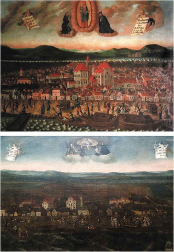
Figure 1. Damage depictions of the city of Komárom (on the left) by Anonymous and (on the right) by Karl Friedl

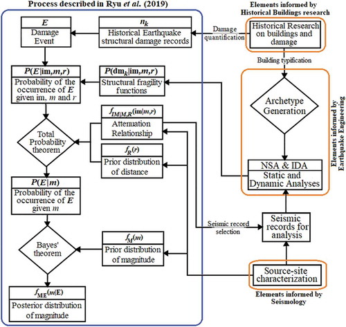
The latter approach relies on a methodology that estimates the magnitude of historical earthquakes using fragility functions and seismic damage records (Figure 2) and it was firstly introduced by Ryu, Kim, and Baker (2009) in the study of the 1613 Seoul earthquake. The study utilized Incremental Dynamic Analysis (IDA; Vamvatsikos and Cornell 2002) for the analysis of a wooden frame associated to the buildings damaged by the 1613 earthquake. Similarly, the FEMA multi-hazard loss estimation methodology HAZUS MH MR1 (2003) also develops seismic fragilities of structural archetypes, or “structures that fairly represent the range of configurations and properties of the building group of interest”. Although, these fragilities are based on the Capacity Spectrum Method (CSM; Freeman 1998) and on archetype categories befitting rather modern Unreinforced Masonry (URM) building typologies. Additionally, studies with reference on Dynamic Structural Analysis (DSA) of URM buildings have questioned the reliability of Nonlinear Static Analysis (NSA) based procedures, as the CSM and the N2-method (EN 1998–1, 2004; Fajfar 1999, 2000). Nakamura et al. (2017) studied the effects of flexible diaphragms stiffness and eccentricity. Guerrini et al. (2017) and Marino, Cattari, and Lagomarsino (2018) additionally studied the dissipated hysteretic energy as a means to predict the inelastic displacement demand, evidencing the difficulty of predicting the behaviour of URM structures with periods lower than 0,25s. Azizi-Bondarabadi, Mendes, and Lourenço (2019) studied further the higher mode effects and progressive damage. The differences exist due to the simplified nature of the NSA procedures, which may not account for the inertial nature of seismic forces in the detailed model together with the duration of the earthquake, cyclic degradation and damage progression. The alternative detailed DSA requires relatively more computation time, which increases with the complexity of the structural model. Despite finer considerations, the studies demonstrate a general tendency of the N2-method to overestimate the strength of URM buildings.

Figure 2. Flowchart of the method for the estimation of the magnitude of historical earthquakes using NSA and IDA of buildings archetypes in relation to historical building research and seismology

The Hungarian building stock of the 18th c. was majorly constituted by regular URM buildings, with rammed-earth, adobe or burnt clay brick walls and self-equilibrated wooden roofs, known to be sensitive to seismic actions. The literature regarding the study of historical Hungarian vernacular typologies of this period is relatively scarce (e.g., Csicsely 2006) and focused on monumental buildings (e.g., Armuth, Hegyi, and Sipos 2010). International literature on the dynamic behaviour of other typologies of adobe vernacular buildings can be followed, for instance, in Tarque et al. (2014a; 2014b). Therefore, in order to study the 1763 Komárom earthquake, previous work relied on the historical survey of the city of Tata (Istvánfi 1995) and on an in-plane vulnerability index methodology (Lourenço and Roque 2006) to develop a total of eight historical building archetypes befitting the study of the 1763 earthquake (Morais, Vigh, and Krähling 2017, 2018a).

The seismic analysis of the eight archetypes is discussed in this article aiming for the production of fragility functions representing their behaviour. Although, the fact that URM is a highly nonlinear and brittle composite material with different failure modes that may interact, the statistical nature of the archetypes, and the different sources of epistemic and physical and model uncertainties related to the work of modelling their seismic vulnerability poses a challenging task. A possible strategy is to model the buildings using the Equivalent Frame Method (EFM) implemented in Tremuri (Lagomarsino et al. 2013) to generate the pushover curves using NSA. The box behaviour of the archetypes is not endorsed due to the presence of flexible diaphragms, nevertheless the evidence of historical damage related to shear and rocking mechanisms (Figure 1) and expected dominance of directional vibration modes (Morais 2019) justifies the use of the EFM. Afterwards, the N2-method may be employed to produce fragility functions for historical URM buildings (Maio, 2013; Vicente 2008).

Additionally, although the physical uncertainties related to the historical conditions of the material parameters can be modelled using Monte-Carlo simulation (MC), carrying out IDA is still forbidding. Therefore, further simplifications in the process are studied here, by calibrating a simplified macro-model of the archetypes in OpenSEES (McKenna, Scott, and Fenves 2010) for DSA. This model uses a Pinching4 material model simulating their cyclic behaviour and degradation (Lowes, Mitra, and Altoontash 2004) following the strategy employed by Furtado et al. (2015; Furtado, Rodrigues, and Arêde 2015) and Morais, Vigh, and Krähling (2017). Other applications implement the EFM formulation directly in OpenSEES (e.g., Raka et al. 2015). The calibration is carried out using a Genetic Algorithm (GA) routine based on Vigh et al. (2014). Fragility functions are attained with IDA of the simplified model and by the application of the N2-method to the results of NSA. The resulting fragilities are analysed and compared. In the last section, the magnitude estimation methodology is illustrated with an application.

2. Methodology

The methodology underlying the present study (Figure 2) was introduced by Ryu, Kim, and Baker (2009) and it aims either for the estimation or the update of the statistical description of the magnitude M of a historical damaging seismic event E. The method uses the Bayes’ theorem to estimate the posterior distribution of magnitude given the damaging event f_m|E, as in Eq. (1(1) $f_{M|E}\left(m|E\right)=\frac{P\left(E|M=m\right)\times f_M(m)}{P\left(E\right)}=\frac{P\left(E|M=m\right)\times f_M(m)}{\int P\left(E|M=m\right)\times f_M(m)dm}$(1) ), by computing a prior distribution of magnitudes f_M(m) together with the probability of the damaging event given a magnitude P(E|m):

(1) $f_{M|E}\left(m|E\right)=\frac{P\left(E|M=m\right)\times f_M(m)}{P\left(E\right)}=\frac{P\left(E|M=m\right)\times f_M(m)}{\int P\left(E|M=m\right)\times f_M(m)dm}$(1)

where m may assume any magnitude scale, although the moment magnitude M_w is employed here, which is commonly applied to seismic hazard prediction (e.g., Woessner et al. 2015), and P(E|m) contains building damage information.

In turn, the probability of the event given magnitude P(E|M= m) is calculated using the total probability theorem as in Eq. (2)(2) $\begin{array}{rl}& P\left(E|M=m\right)=\int \int P\left(E|im,m,r\right)\times f_{IM|M,R}\left(im|m,r\right)dr\\ & \times f_R\left(r\right)dimdr\end{array}$(2) :

(2) $\begin{array}{rl}& P\left(E|M=m\right)=\int \int P\left(E|im,m,r\right)\times f_{IM|M,R}\left(im|m,r\right)dr\\ & \times f_R\left(r\right)dimdr\end{array}$(2)

where f_IM|M,R describes the attenuation relationship, with intensity measure IM (any measure of the intensity spectrum, normally the one that is relevant for the damage description, here the PGA, in g, or spectral acceleration in the period T_n= 0s is employed) and distance R, f_R the prior distribution of distance, and P(E|im,m,r) the likelihood of the damaging event E based on a specific combination of the occurred damage with fragilities of the type P(DM≥ds_i|im,m,r). The symbols im, m and r denote the discrete occurrences of IM, M and R.

An important step for the estimation of the seismic fragilities is to model and analyse both the behaviour of the buildings, or archetypes, and the seismic demand that are coherent with the damage described in the structural damage records and site location.

2.1. Fragility functions fitting

The estimation of fragility functions provides the probability of occurrence of a certain damage state ds_i given a set of parameters θ that define the ground motion intensity, here intensity measure IM, magnitude M and distance R. In the present study the PGA is utilized as IM. Fragility functions are arguably assumed to be represented by a lognormal (or equivalent normal) cumulative distribution function (CDF):

(3) $P\left(DM\ge d{s}_i|\theta \right)=\mathrm{\Phi }\left(\frac{ln\left(x_{\theta }/{\mu }_i\right)}{{\beta }_i}\right)$(3)

The procedure uses the maximum likelihood estimation of the median μ_i and standard deviation β_i, of the damage intensities PGA_ds,i for different damage states, here i= {1,2,3,4}. In turn, the PGA_ds,i points are estimated with IDA or N2-method procedures associated either to the time-history or NSA analysis of a numerical model representing the nonlinear behaviour of URM buildings and previously selected seismic records. Similar studies in literature have endorsed fragility databases, as in Silva, Crowley, and Colombi (2014).

2.2. Detailed macro-modelling and analysis

The EFM implemented in Tremuri (Lagomarsino et al. 2013) has been an efficient tool to model the nonlinear static and dynamic behaviour of URM buildings, based on the in-plane rocking and shear behaviour of piers and spandrels (or lintels) connected by 2D and 3D rigid nodes (Figure 3). In order to highlight the mechanical variability, the present paper does not address the EFM formulation in detail, only the general relations between the respective variables. More details can be read in the literature (Lagomarsino et al. 2013) and Tremuri manual (Lagomarsino et al. 2008).

Figure 3. Sketch of the idealization of masonry pier response by adopting simplified strength criteria based on applied axial compression force

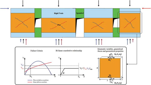
The piers and lintels can be modelled with 2D beam elements with a bilinear material model, conditioned both by rocking and shear Mohr-Coloumb or Turnšek-Cacovic yielding criteria (Figure 3). The kinematics of the 2D beam model for piers and lintels are described by a 6 degree-of-freedom array a^T ={u_i w_i φ_i u_j w_j φ_j}. Here, u and w are the transversal and axial translations and φ is the rotation of the node i or j. The 2D element is defined by a deformable height h, length l and thickness t. The internal forces corresponding the deformation are the shear force V, normal force N, and bending moment M, for the same nodes i and j. The internal forces F = {V_i N_i M_i V_j N_j M_j} corresponding the deformation are the shear force V, normal force N, and bending moment M, for the same nodes i and j. The linear elastic branch is defined by a constitutive relationship F = K∙d, where the stiffness matrix K is a function of the Young and shear moduli, respectively E and G, the cross-sectional area A, the moment of inertia I, and a stiffness reduction coefficient η, aiming to account for the stiffness cyclic degradation, defined in relation to the σ₀/f_m relationship (Lagomarsino et al. 2013).

The ultimate values of the nodal forces can be determined as a function of the normal stresses σ₀, compressive strength f_m, and its horizontal value f_h, shear strength of the piers and lintels, respectively f_vk0 and τ₀, ft is the strength of the stretched interposed element inside the lintel, and of the ultimate shear and bending drift ratios, δ_u,v and δ_u,r respectively. The expressions to calculate the ultimate force and displacement values act as conditions for the nonlinear and complex behaviour of the detailed models of the archetypes, under the effect of either seismic static or dynamic loading. The following subsection addresses a simplification process that uses only the force-displacement diagrams obtained from detailed NSA for nonlinear dynamic analysis.

2.3. Simplified macro-modelling and calibration

The structural model utilized for the calibration process was proposed and implemented in OpenSEES by Furtado, Rodrigues, and Arêde (2015) for masonry infill walls and it was later adapted by Morais, Vigh, and Krähling (2017) for individual URM panels. The model consists of an isostatic 2D frame, composed by infinitely rigid frames connected by a linking element (Figure 4) modelled with a pinching4 multilinear uniaxial material model with cyclic degradation (Lowes, Mitra, and Altoontash 2004).

Figure 4. OpenSees model (up left) backbone parameters of the “pinching4” uniaxial material model (up right) and cyclic degradation models (down), based on Lowes, Mitra, and Altoontash (2004)

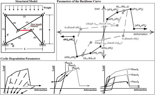
The pinching4 material model has 39 material model parameters (see Table 1). While the first 16 can be calibrated by idealizing the monotonic F-δ diagram, the others are related to the cyclic behaviour and degradation and, therefore, are calibrated from the hysteretic curve (Figure 4). The degradation parameters can be calculated for each time-step i:

(4) $\begin{array}{rl}& {\delta }_i={\alpha }_1{\left({\tilde{d}}_{max}\right)}^{{\alpha }_3}+{\alpha }_2{\left(\frac{E_i}{E_m}\right)}^{{\alpha }_1}\le {\alpha }_{Lim},{\tilde{d}}_{max}\\ & =max\left\{\frac{d_{max,i}}{de{f}_{max}},\frac{d_{min,i}}{de{f}_{min}}\right\}\mathrm{\&}{E}_i=\underset{\hspace{0.17em}}{\int }dE\end{array}$(4)

Table 1. List of parameters associated to the Pinching4 material model (McKenna et al., 2010; Lowes et al., 2004)

Parameters	Number	Description
ePfi	4	Force points of the positive envelope
ePdi	4	Deformation points of the positive envelope
eNfi	4	Force points of the negative envelope
eNdi	4	Deformation points of the negative envelope
rDispP	1	Ratio of the force at which reloading begins to force corresponding to the maximum historic deformation demand
fForceP	1	Ratio of strength developed upon unloading from negative load to the maximum strength developed under monotonic loading
uForceP	1	Ratio of the deformation at which reloading occurs to the minimum historic deformation demand
rDispN	1	Ratio of the force at which reloading begins to force corresponding to the minimum historic deformation demand
fForceN	1	Ratio of the force at which reloading begins to force corresponding to the minimum historic deformation demand
uForceN	1	Ratio of strength developed upon unloading from negative load to the minimum strength developed under monotonic loading
gKi, gKLim	5	Unloading stiffness degradation
gDi, gDLim	5	Reloading stiffness degradation
gFi, gFLim	5	Strength degradation
gE	1	Maximum energy dissipation under cyclic loading
dmgType	1	Type of damage (option: “cycle” or “energy”)

where δ_i is the damage index (ranges between 0 and 1), α_i corresponds to the parameters gKi, gF_i, and gD_i used to fit the damage rule to the experimental data. The parameter E_i is the hysteretic energy and E_m is the energy that is required to achieve the deformation that defines failure under monotonic loading. The def_max and def_min are, respectively, the positive and negative deformations that define failure, and d_max,i and d_min,i are, respectively, the maximum and minimum historic deformation demands.

In turn, the damage indices δ_i can be determined for the cases of stiffness and strength degradation and the increase in historic deformation, using Eq. (5)(5) $X_i=X_0\cdot \left(1-{\delta }_i\right)$(5) .

(5) $X_i=X_0\cdot \left(1-{\delta }_i\right)$(5)

where X_i is the set defined by the current unloading stiffness k_i, the current envelope maximum strength f_max,_i and current deformation that defines the end of the reload cycle for increasing deformation demand d_max,i,; X₀ is the set defined by the initial unloading stiffness for the case of no damage k₀, f_max,0 is the initial envelope maximum strength for the case of no damage and d_max,0 the maximum historic deformation demand.

One alternative to calibrate the parameters of the material models has been to employ a Genetic algorithm (GA) in order to obtain an optimal set of values (Vigh et al. 2014). The algorithm evolves from an initial population by evaluating the fitness of successive generations of individuals generated by mutation. Following the nomenclature of genetics, the algorithm regards the individuals as phenotypes defined by chromosomes (sets of parameters), which are composed of alleles (parameters’ values). The iterative process is concluded with the fittest individuals evaluated by a fitness function and under stopping criteria.

The development of the detailed models is described in section 3, while the simplified model and calibration process for the IDA analysis in OpenSEES will be more thoroughly described in section 4.

3. Structural modelling, uncertainties and sampling

The present section discusses the processes of modelling and NSA of the eight archetypes, A0 to A7, using the EFM implemented in Tremuri. The geometrical properties, main structural elements, mechanical parameter inputs of the archetypes are highlighted, as well as the load model and uncertainties related to these parameters are also presented. Although the modelling uncertainties associated to the EFM are not addressed here in particular, it has been shown to provide relatively conservative results, in the light of comparative studies (Rota, Penna, and Magenes 2014; Sevieri et al. 2017).

3.1. Geometrical and structural modelling

The building archetypes under analysis representing the historical buildings stock of 18th c. Komárom totalize eight geometries associated to four different buildings classes: class 1, composed by A0 (pilot version) to A2; class 2, by A3; class 3, by A4 and A6; and class 4, by A5 and A7. They were computed and discretized in Tremuri environment (Lagomarsino et al. 2013) into detailed macro-models. Their geometrical parameters and structural models can be seen in Table 2 and Figure 5, respectively.

Table 2. Input geometrical parameters for the building archetypes A0 to A7 (Figure 5)

	Geometrical Parameters												Openings
Archetypes	L1	L2	L3	L4	L5	L6	L7	t1	t2	h1	h2	h3	Front-doors	Inner-doors	Windows
A0	4.70	2.80	3.80	4.70	-	-	-	0.50	-	2.60	2.00	-	0.90 × 2.00	0.80 × 2.00	0.70 × 1.00
A1	4.70	2.80	3.80	4.70	-	-	-	0.55	-	3.00	2.50	-
A2	4.50	4.50	3.50	4.50	4.50	5.00	2.50	0.55	0.55	3.00	2.50	-	1.30 × 2.00	1.10 × 2.00	0.90 × 1.00
A3	4.50	4.50	3.50	4.50	4.50	5.40	2.50	0.73	0.73	3.20	3.00	-
A4	4.80	4.80	3.80	4.80	4.80	6.20	3.25	0.96	0.96	3.63	3.20	-	1.40 × 2.50	1.30 × 2.50	1.30 × 1.50
A5	4.80	4.80	3.80	4.80	4.80	6.20	3.25	0.96	0.96	4.16	3.50	-	-	-
A6	5.95	3.25	4.45	4.45	-	-	-	0.73	-	3.20	3.20	6.40	1.45 × 2.00	1.10 × 2.00	1.00 × 1.00
A7	5.49	4.57	3.66	4.57	5.49	4.57	4.57	0.96	0.96	3.63	3.63	3.63	1.65 × 3.00	1.25 × 3.00	1.65 × 2.00

Figure 5. Historical building archetypes modelled in Tremuri, typologies A0 and A1 (on the left), A2, A3, A4 & A5 (on the center left), A6 (on the center right) and A7 (on the right)

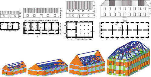
Figure 6. Adobe, mud or rammed-earth buildings in the Hungarian Kingdom, from Csicsely (2006)

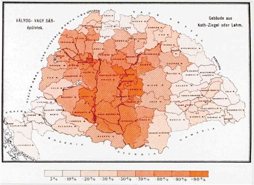
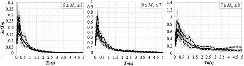
Figure 7. Ground motion spectra (mean ± standard deviation) selected for ranges of magnitude and distance

The archetypes are low-rise URM buildings, generally regular both in plan and in height. The roof systems are typical from the baroque period, self-equilibrated and varying from simply trussed to mansard wooden tiled roofs with open gables (see also Figure 1), except for the hipped roof of A7. The cross-sections of the wooden beams and floors also vary from around 0.18 to 0.32 m, imparting the roof weight to the self-supporting walls which constitute the main resisting system of the URM archetypes. According to earlier studies on the dynamics of the assemblies, the roof and floors were observed to provide considerable horizontal rigidity, despite their relative flexibility, resulting in a coupling effect in the behaviour of the walls (Morais 2019). The material parameters utilized in the modelling process are described in the following subsection.

3.2. Material strength parameters

The strength parameters were arguably organized in accordance to the four major building classes and considering that probably more than 80% to 90% of the buildings in the 18th c. were made of mud, rammed-earth and adobe, according to the (end of) nineteenth century map by Posner Károly Lajos & Son (Figure 6), from Csicsely (2006).

This data updates previous work (Morais, Vigh, and Krähling 2018a, 2018b) on the knowledge of the building materials and respective strength. The study of the variety of both historical materials and buildings in Hungary is ongoing and the study of their resistance is still rare in literature. Therefore, the strength parameters were defined with basis on international literature on adobe and mud URM presented in works by Csicsely (2006) and Caporale et al. (2015), and the burnt brick masonry by Zimmermann, Strauss, and Bergmeister (2010). See also Tarque et al. (2014a; 2014b) for a thorough discussion on the dynamic behaviour of adobe URM and respective parameters.

The parameters for the Mohr-Coulomb material model utilized to model the eight archetypes in Tremuri and the respective categories are presented in Table 3, where γ is the specific weight, f_m the masonry compressive strength, f_v the shear strength, δ_u,v and δ_u,f the shear and flexural drift ratios, respectively. The shear modulus G, in this study, is calculated by the expression E/(2(1 + ν)), as a function of the Young’s modulus E and Poisson’s ratio ν. The use of this expression is associated to the original condition of the URM buildings (e.g., EN 1996- 1-1 2005). Nevertheless, it is noteworthy to mention that the E/G ratio of existing adobe walls may vary in a wider range—e.g., between 2.38 and 6.60 (Tarque 2008)—and the application of the E/G ratio may be studied in future works. Additionally, the wooden elements were assumed as a relatively soft C14 pine, with γ = 5,0 kN/m³, E = 11,0 GPa and ν = 0.30.

Table 3. Physical and strength parameters for the archetypes A0-to-A7 in four major classes, mean and standard deviation in brackets

Building classes	1	2	3	4
Archetypes	A0, A1 & A2	A3	A4 & A6	A5 & A7	Distribution type
γ [kN/m^3]	16.0(-)	17.0(-)	17.0(-)	18.0(-)	Deterministic
E [MPa]	155(100)	200(50)	350(100)	1375(500)	Lognormal
ν [-]	0.20(0.05)	0.20(0.05)	0.20(0.05)	0.20(0.05)	Normal
fm [MPa]	1.00(0.75)	1.50(0.90)	2.35(1.00)	4.00(1.50)	Lognormal
fvk0 [MPa]	0.09(0.015)	0.10(0.07)	0.50(0.10)	0.35(0.10)	Lognormal
G(E,ν) [MPa]	64.58(-)	83.33(-)	145.83(-)	572.91(-)	Expression
δu,v [%]	0.53(0.16)	0.53(0.16)	0.53(0.16)	0.53(0.16)	Normal
δu,f [%]	1.07(0.43)	1.07(0.43)	1.07(0.43)	1.07(0.43)	Normal

3.3. Load modelling

The seismic load model utilized follows Eurocode 8 (EN1998-1, 2004) and considers G and Q the nominal values of permanent and live loads, with Ψ_E·Q the quasi-permanent loading, A_E the design seismic actions, in the load combination ΣG_j “+” A_E “+” Σψ_E,i·Q_i. While the permanent loads are defined by the weight of the structural elements, the live load depends on the building and storey category as well as the live-load reference values. In turn, the seismic load A_E is defined by ground motion records and earthquake spectra selected for Komárom, using PEER database (2013). The ground motion model and epistemic uncertainties were incorporated using a logic tree defined by two ground motion prediction models (GMPE) utilized both for SHARE hazard model (Woessner et al. 2015) and Paks II nuclear power plant (MVM Paks II Ltd 2016) with equal weights of 0.5. The site classification assumes the predominance of C2t (45%) and B1b (40%), followed by C3t (10%) and C2b (5%), according to Kiss (2017) and Pitilakis (2004). Three different bins of real GM records (10 each) were finally selected (Figure 7) following Ryu, Kim, and Baker (2009), with different magnitude ranges 5 ≤ M_w< 6, 6 ≤ M_w< 7 and 7 ≤ M_w < 8, distance 0 ≤ R_JB< 25, assuming strike-slip fault.

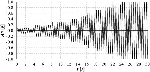
In addition, a cyclic loading protocol was created based on Krawinkler (2009). Its normalized version (with PGA = 1.0 g), in Figure 8, is multiplied by a factor such that PGA = PGA_ds4, hence, describing the full hysteretic curve until collapse. The analysis process and respective results are described in 4.1.

Figure 8. Normalized load protocol with increasing load steps (Krawinkler 2009)

3.4. Statistical sampling

The different archetypes A0 to A7 aim to represent the wide range of building categories and typologies existing in the 18th c. in the county of Komárom. Their specific geometrical configurations represent geometric variability, the uncertainty in both seismic demand and resistance are accounted for through the variability of the GM records, in different bins, and the mechanical parameters are shown in subsection 3.2. The characterization of the physical uncertainty expressed in the variability of the mechanical parameters is strictly related to the present analysis strategy, because the NSA using the EFM requires less computation time than the DSA. Hence, the model simplification strategy suggested in subsection 2.3 uses not only the NSA of the archetypes based on a sampling technique but also the properties of their dynamic behaviour, namely the cyclic degradation. While the latter issue is addressed in the following section, a Monte-Carlo (MC) simulation technique is employed to generate the sets of input strength parameters, following the moments and distributions presented in Table 3.

(6) ${\theta }_i=\left\{ln(E),\nu ,ln(f_m),ln(f_{vk0}),{\delta }_{u,v},{\delta }_{u,f}\right\}\sim N_j\left({\mu }_i,{\sigma }_i\right)$(6)

where the set θ_i of i input parameters is approximated by a N_j normally distributed set of parameters, with j ={1 … N_spl}, N_spl being the number of samples; μ_i and σ_i the mean value and standard deviation of the i^th parameter, respectively.

4. Nonlinear static and dynamic analyses and calibration

Despite the relatively high efficiency of the present models for NSA, the computation demand is still forbidding in the case of IDA, mainly due to the number of samples necessary for MC simulation. This section addresses the analysis and calibration processes.

4.1. Static vs dynamic analysis

The process of calibration of the simplified macro-model described in 2.3 requires the knowledge of the dynamic behaviour of the archetypes, first under monotonic loading and then, to understand the cyclic degradation, under cyclic loading. Thus, the nonlinear static and dynamic analyses were carried out, using static force and displacement based pushover procedures and then a dynamic cyclic loading protocol (Figure 8), respectively, in both x and y directions independently and for the average values of the parameters in Table 3. The hysteretic curves from the time-history analysis are presented in Figure 9, while the backbone curve from the dynamic analysis is compared with the pushover curves in Figure 10.

Figure 9. Results for the dynamic analysis of the Archetypes (hysteretic curve in blue) and respective backbone (in black), from A0-to-A7 and in both x and y directions

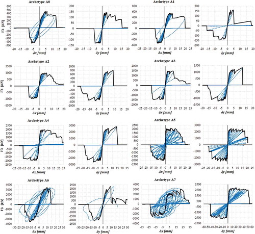
Figure 10. Comparison between NSA: force (in blue) and displacements (in orange) based procedures, and the backbone from DSA (in black)

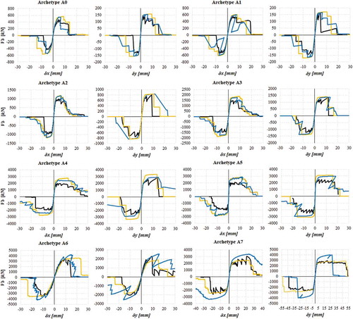
The results show the proximity of the curves in different analyses, although some discrepancies exist, namely in the post-peak trench—when δ > δ(F_máx)—and in the maximum and ultimate displacements, despite the usual agreement in the maximum force. The displacement δx and δy are utilized as demand parameter for simplicity, since they are also the control parameters for the pushover analysis and can be directly translated to damage limit states. For this reason and to maintain the efficiency of the approach, a static monotonic load protocol is not employed here for the calibration of the cyclic parameters. It is also argued that the proximity between the displacement based pushover and dynamic backbone curves is held due to the relative regularity, low height and existence of a flexible diaphragm provided by the roof structure. The calibration procedure is explained in the following subsection.

4.2. The calibration using a genetic algorithm

One important remark regarding the calibration process and this particular strategy is that the simplified model emulates the hysteretic behaviour of the model of reference (or experiment) in its level of detail, using the Pinching4 material model. In the present case, the EFM models, the stiffness degradation trough the stiffness reduction coefficient and, therefore, the strength and reloading stiffness degradation (resulting in additional deformation demand) can be here neglected, thus gF_Lim = 0 and gD_Lim = 0. In turn, the symmetry between positive and negative sides of the hysteretic curve results that ePf_i = eNf_i, ePd_i = eNdf_i, rDispP = rDispN, fForceP = fForceN and uForceP = uForceN. In addition, the monotonic curves (from NSA) provide the points (ePd_i, ePf_i): ePd₁ = δ_y, ePd₃ = δ_max, ePd₄ = δ_ult, ePd₂ = (δ_y+δ_max)/2, and similarly, ePf₁ = F_y, ePf₃ = F_max, ePd₄ = F_ult, ePf₂= F(δ = ePd₂). Here, F_y can be determined by adopting a criteria of equal collapse energy and by assuming that the ultimate displacement δ_ult is the displacement associated to the residual strength F_ult. These particular considerations reduce the number of calibration parameters from 37 to 8.

The objective and fitness functions were defined based on the optimization strategy in Eq. (7)(7) $F_{obj}=\sum _{i=1}^n{\left[k_{2,i}{\left(F_{est,i}-F_{exp,i}\right)}^{k_1}\right]}^2\mathrm{\&}Fitness=\frac{{10}^{15}}{F_{obj}}$(7) . The parameters assume the values k₁ = 1 and k_2,i = |δ_i|/2, and F_est,i and F_exp,i are the estimated and reference forces, respectively. The strategy for the selection of the calibration points (δ_i, F_exp,i), despite Vigh et al. (2014), only considers mid- and end-points in the loading/reloading cycles due to the low dissipation of energy in the unloading process. Otherwise, the mid-points in loading and unloading could be mistaken because of their proximity.

(7) $F_{obj}=\sum _{i=1}^n{\left[k_{2,i}{\left(F_{est,i}-F_{exp,i}\right)}^{k_1}\right]}^2\mathrm{\&}Fitness=\frac{{10}^{15}}{F_{obj}}$(7)

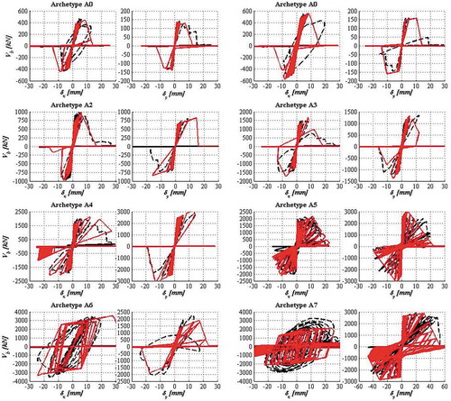
The GA-based calibration pushover routine based on displacement increments was set with initial population and upper and lower bounds, uniform selection and mutation, and heuristic crossover. After a maximum of 100 generations, the calibration routine produced similar populations of 30 individuals. While the optimized curves are in Figure 11, the fittest individuals are presented in Table 4.

Table 4. Cyclic degradation parameters for ‘Piching4ʹ model of the archetypes A0 to A7, and respective fitness grade

Archetypes	Dir.	rDisp	fForce	uForce	gK1	gK2	gK3	gK4	gKlim	Fitness
A0	x	0.09	0.07	−0.91	0.04	0.06	1.82	2.00	0.97	9 × 10^8
	y	0.03	0.09	−0.90	0.81	0.38	0.36	0.99	0.70	10^12
A1	x	−0.09	0.10	−0.90	0.33	0.88	0.91	0.21	0.84	7 × 10^7
	y	0.06	0.06	−0.96	0.53	0.33	0.36	0.76	0.95	5 × 10^9
A2	x	0.10	−0.03	−0.71	0.94	0.81	1.86	1.14	0.71	10^10
	y	0.09	0.07	−0.98	0.71	0.91	0.96	0.41	0.66	5 × 10^9
A3	x	0.09	−0.04	−0.95	0.05	0.41	1.96	1.92	0.63	2 × 10^8
	y	−0.02	0.06	−0.98	0.97	0.45	0.63	0.38	0.84	3 × 10^7
A4	x	0.10	0.00	−0.92	0.92	0.52	0.10	0.35	0.68	6 × 10^6
	y	0.01	0.01	−0.93	0.10	0.76	1.40	0.64	0.66	3 × 10^8
A5	x	0.10	0.03	−0.91	0.53	0.99	0.05	0.31	1.00	6 × 10^6
	y	−0.04	0.10	−0.95	0.34	0.94	0.97	0.71	0.99	5 × 10^5
A6	x	0.24	0.99	0.58	0.52	0.63	0.63	0.83	0.60	2 × 10^6
	y	−0.09	0.10	−0.92	0.38	0.82	1.21	0.02	0.71	3 × 10^6
A7	x	−0.29	−0.33	0.70	0.29	0.86	0.42	0.41	0.61	2 × 10^6
	y	−0.04	−0.04	−0.90	0.04	0.02	1.96	1.97	0.93	10^5

Figure 11. Cyclic procedure F-δ diagrams (in black) and fittest individuals (in red) obtained with GA, for the Archetypes, from A0 to A7, and directions x and y.

4.3. The N2-method and data for seismic analysis

The seismic analysis was carried out with the N2-method and DSA using the ground motion inputs selected in 3.3. The IDA uses an incremental scaling procedure over the GM intensities, such that PGA_i = PGA_i-1+ dPGA, for i= {1 … n}, where n means the collapse of the structure, when δ_n≥δ_ult = ePd₄. This process entails that the intensity points were collected at different damaging intensity levels PGA_ds,i, associated to the four damage limit states ds_i, defined in terms of displacements and associated to the simplified model, such that δ_ds,i = ePd_i.

The N2-method is widely known and accessible in the Appendix B of the Eurocode 8 (EN1998-1, 2004) and utilizes the dynamic properties of the structures such as the transformation factor Γ and the reduced mass m* to reduce the MDOF system to an equivalent bilinear SDOF system, with normalized forces F* = F_b/Γ and displacements δ* = δ_n/Γ. The archetypes are generally low-rise buildings with one or two storeys, governed by the first mode and have modal mass ratios in the range of 70 ~ 80% (Morais 2019), and therefore the normalized displacement vectors are assumed either as Φ = 1.0 or Φ = [0.5 1.0]. The masses of the archetypes are given in tons, in the set M_Ai = {104.20, 137.32, 330.88, 522.23, 900.35, 1016.60, 794.90, 1865.50}, from A0 to A7.

The N2-method assumes the equivalence of energy in order to calculate the bilinear capacity curve for a given point, with force F_y* and deformation δ_m*. As a result, both the yielding deformation δ_y*, fundamental period of the SDOF system T* and the target displacement of the linear elastic SDOF δ_et* can be calculated for each structure by transformation. Additionally, the damage points δ_ds,i are known from the pushover curves, as described in 4.2, and the elastic response spectrum S_e(T) is known for each of the GM records.

Thus, the target displacement of the equivalent SDOF δ_t* can be calculated using Eq. (8)(8) ${\delta }_t^{\ast }=\left\{\begin{array}{cc}\frac{{\delta }_{et}^{\ast }}{q_u}\left(1+(q_u-1)\frac{T_C}{T^{\ast }}\right)& \mathrm{i}\mathrm{f}{T}^{\ast }<T_C\\ {\delta }_{et}^{\ast }& \mathrm{i}\mathrm{f}{T}^{\ast }\ge T_C\end{array}\right.$(8) as follows:

(8) ${\delta }_t^{\ast }=\left\{\begin{array}{cc}\frac{{\delta }_{et}^{\ast }}{q_u}\left(1+(q_u-1)\frac{T_C}{T^{\ast }}\right)& \mathrm{i}\mathrm{f}{T}^{\ast }<T_C\\ {\delta }_{et}^{\ast }& \mathrm{i}\mathrm{f}{T}^{\ast }\ge T_C\end{array}\right.$(8)

where the ductility factor q_u is calculated as S_e(T*)m*/F_y*≥1.0. The corner period T_C can be calculated for each GM record as T_C = 2π×EPV/EPA, being EPA and EPV the mean spectral accelerations and velocities, respectively, in an interval ΔT= 0.40s around their maximum values. Finally, the target displacement of the MDOF can be calculated by back-transformation as δ_t = Γ·δ_t*, associated to each of the damage states of the structure.

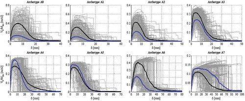
The base shear forces F_b of the force-displacement diagrams obtained from NSA of the archetypes with N_spl = 100 were then divided by M_Ai, providing a rough draft of the seismic capacity and what can be expected from the fragilities (vide Figure 12). The results obtained with the application of the N2-method and DSA are presented and discussed in the following section, in terms of fragility functions.

Figure 12. Force displacement diagrams obtained from NSA of the Archetypes (in grey), from A0-to-A7, and respective means for directions x and y (in black and blue, respectively)

5. Analysis of the results

Although the damage itself detailed by Morais (2019) is not addressed in this paper, the damage limit states were defined. Therefore, the damaging intensities PGA_ds,i, collected after the NSA and IDA procedures, can be adjusted to lognormal curves with moments μ_i and β_i, as in Eq. (3)(3) $P\left(DM\ge d{s}_i|\theta \right)=\mathrm{\Phi }\left(\frac{ln\left(x_{\theta }/{\mu }_i\right)}{{\beta }_i}\right)$(3) . This section presents and discusses the results from the static and dynamic analyses.

5.1. The N2-method vs dynamic structural analysis

While the N2-method approach utilized the capacity curves obtained from the NSA together with the earthquake spectra from the selected GM records in a static procedure (explained in 4.3), the DSA employed the GM records and the simplified dynamic model with the pinching4 material. The fragility functions obtained from the static procedure are shown in Figure 13, while the respective moments are displayed in Table 5. Additionally, the fragilities obtained from the dynamic procedure are provided in Figure 14, with the respective moments in Table 6.

Table 5. Fragility moments for the archetypes A0 to A7 using N2-method

		Direction x				Direction y
Archetype	Moments	1	2	3	4	1	2	3	4
A0	μdsi	0.113	0.272	0.336	0.395	0.042	0.135	0.185	0.229
	βdsi	0.618	0.420	0.422	0.394	1.022	0.403	0.446	0.443
A1	μdsi	0.128	0.207	0.246	0.304	0.051	0.109	0.153	0.184
	βdsi	0.488	0.448	0.433	0.368	0.390	0.377	0.402	0.425
A2	μdsi	0.092	0.167	0.210	0.262	0.047	0.122	0.180	0.195
	βdsi	0.416	0.401	0.382	0.354	0.572	0.419	0.412	0.412
A3	μdsi	0.149	0.297	0.364	0.419	0.126	0.249	0.335	0.370
	βdsi	0.425	0.371	0.350	0.305	0.331	0.370	0.387	0.360
A4	μdsi	0.150	0.302	0.372	0.459	0.187	0.359	0.470	0.506
	βdsi	0.332	0.310	0.311	0.331	0.260	0.315	0.349	0.327
A5	μdsi	0.201	0.326	0.372	0.423	0.214	0.513	0.656	0.685
	βdsi	0.399	0.329	0.282	0.282	0.342	0.475	0.462	0.428
A6	μdsi	0.213	0.360	0.451	0.514	0.101	0.195	0.258	0.304
	βdsi	0.323	0.305	0.318	0.320	0.286	0.299	0.324	0.329
A7	μdsi	0.019	0.162	0.263	0.341	0.071	0.298	0.459	0.504
	βdsi	0.732	0.371	0.379	0.406	0.287	0.432	0.464	0.455

Table 6. Fragility moments for the archetypes A0 to A7 using IDA

		Direction x				Direction y
Archetypes	Moments	1	2	3	4	1	2	3	4
A0	μdsi	0.079	0.122	0.185	0.280	0.065	0.091	0.126	0.185
	βdsi	0.707	0.680	0.634	0.656	0.721	0.613	0.561	0.569
A1	μdsi	0.077	0.151	0.198	0.244	0.060	0.105	0.131	0.163
	βdsi	0.944	0.845	0.838	0.792	1.008	0.874	0.811	0.735
A2	μdsi	0.032	0.044	0.063	0.133	0.018	0.026	0.035	0.076
	βdsi	0.967	0.760	0.740	0.896	1.130	0.853	0.737	0.875
A3	μdsi	0.090	0.128	0.153	0.400	0.078	0.103	0.116	0.262
	βdsi	0.702	0.896	0.951	0.511	0.700	0.802	0.799	0.375
A4	μdsi	0.068	0.109	0.134	0.438	0.057	0.085	0.100	0.283
	βdsi	0.563	0.790	0.891	0.561	0.473	0.658	0.713	0.415
A5	μdsi	0.097	0.151	0.180	0.478	0.109	0.140	0.158	0.344
	βdsi	0.883	1.145	1.170	0.531	1.058	1.116	1.085	0.538
A6	μdsi	0.308	0.493	0.573	0.593	0.244	0.350	0.386	0.398
	βdsi	0.595	0.547	0.549	0.538	0.468	0.447	0.443	0.432
A7	μdsi	0.056	0.242	0.336	0.362	0.052	0.178	0.232	0.251
	βdsi	0.689	0.611	0.631	0.613	0.757	0.599	0.580	0.552

Figure 13. Seismic fragility functions for four sequential damage states (slight in green, moderate in blue, severe in orange, and total damage in red) using the N2-method approach

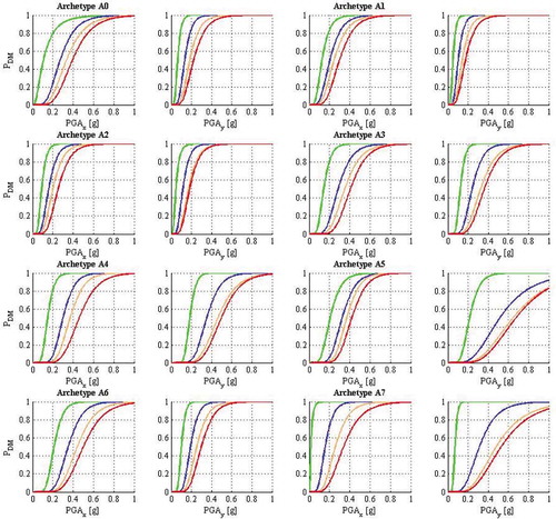
Figure 14. Seismic fragility functions for four sequential damage states (slight in green, moderate in blue, severe in orange, and total damage in red) using the IDA approach

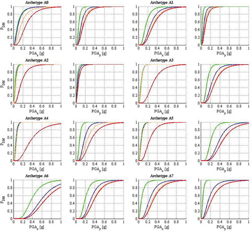
Important discrepancies arose between the N2 and IDA results, although, the differences resulting from the number of samples (N_spl= 100 and 1000 were tested) are below 5% maximum within the analysis methodology. The fragilities developed by IDA provide lower damage intensities when compared to those obtained by the N2-method. The union of the sets of damaging intensities, from A0 to A7, enforces this remark, as for N2-method the resulting medians are μ_i= {0.104 0.290 0.401 0.451} with standard deviations β_i= {0.778 0.612 0.591 0.551}. The medians, for IDA, are μ_i= {0.074 0.126 0.158 0.273} and standard deviation β_i= {1.029 1.042 1.020 0.801}.

These discrepancies may be partially explained by the fact that the latter approach disregards GM duration and cyclic degradation, since the computation of the degradation in IDA strongly reduced the damaging intensities PGA_ds,i. This is a relevant aspect for structures with the low dissipation capacity of URM. Another important aspect is that the simplification of the structural model for IDA entails that the capacity curves obtained with NSA represents the real dynamic behaviour of the same structures with the discrepancies reported in literature (see Azizi-Bondarabadi, Mendes, and Lourenço 2019; Guerrini et al. 2017; Marino, Cattari, and Lagomarsino 2018; Nakamura et al. 2017). Globally, the normalized error within archetypes varied in between 1% and 106%, and it has a maximum of 45% if the set of archetypes (A0 to A7) is considered instead. Another important remark on the IDA procedure is the difficulty in distinguishing the PGA_ds,i values associated to the damage states ds₃ and ds₄ in the process of data points collection. This fact is associated to the brittle behaviour of the URM that results on a sudden drop after the peak strength (e.g., backbone in Figure 9, A0, dir. x), which sometimes justified the assumption that PGA_ds3= PGA_ds4.

5.2. Discussion of the results

Although nonlinear time-history is usually preferred to NSA (EN1998-1, 2004), NSA has been employed with the N2 method for the seismic vulnerability and risk analysis of historical buildings (Maio et al. 2016; Vicente 2008). In those regards, efficiency opposes detail.

The simplification process conducted in OpenSEES aimed to ally the efficiency of the simplified model to the detail of the damage analysis and force-displacement diagrams provided by the NSA of the archetypes using the EFM in Tremuri. For that purpose, the simplified models employed for IDA were calibrated with cyclic degradation parameters obtained by comparing hysteretic and pushover curves of the same archetypes. This aspect differs from the studies conducted by Nakamura et al. (2017) Guerrini et al. (2017), Marino, Cattari, and Lagomarsino (2018) and Azizi-Bondarabadi, Mendes, and Lourenço (2019), where NSA and IDA procedures were applied to the same structural models. That strategy was not followed here due to the unfeasible computational demand. As a result, the differences between the fragilities obtained with the N2-method and the IDA are grounded not only on the cyclic degradation and earthquake duration considered in IDA, but also on how the NSA (pushover) simulates the damage progression.

The above-mentioned studies conclude that the EFM allied to the N2-method provide non-conservative results (see also, e.g., Silva, Crowley, and Colombi 2014) on irregular low-rise and short-period URM buildings with flexible diaphragms. That statement is consistent with the results obtained from the present study, since the DSA of the calibrated model (with cyclic degradation) imposes a global reduction of the damaging intensities PGA_ds,i. Nevertheless, more refined conclusions require further studies and more detailed comparisons.

Furthermore, the expected outcome in the magnitude estimation of the 1763 earthquake is that the static approach leads to higher estimates than the dynamic approach. The application of the magnitude estimation method is carried out in the following section.

6. Application of the fragility assessment: magnitude estimation

The basic elements for the estimation of the magnitude of the 1763 Komárom earthquake have been introduced in section 2, the attenuation model was presented in subsection 3.3 and the fragilities were attained and discussed in section 5. This section presents a simple case application of the fragilities in the estimation of the magnitude, illustrating the importance of the fragility functions in the magnitude estimation process.

6.1. Damage records and prior distributions

The 1763 Komárom earthquake was the most destructive historical seismic event that affected the current Hungarian territory in the last 300 years. It is reported to have damaged 91% of the buildings in the free city of Komárom (Figure 1): out of 1169 houses in total, 279 ended completely destroyed, 353 partially collapsed, 213 needed expensive repair and 219 cheap repair (Varga, Szeidovitz, and Gutdeutsch 2001).

The epicenter of the earthquake has been estimated to be close to the Raba-Hurbanovo tectonic line, approximately in 17.958º/47.802º, 10 to 12 km from Komárom, considering the damage reports for the Komárom county (Morais 2019; Varga, Szeidovitz, and Gutdeutsch 2001). As a result, both distance and prior magnitude distributions are set following the Eq. (9)(9) $f_R(r)=\frac{2r}{r_u^2-r_l^2}\mathrm{\&}{f}_M(m)=\frac{1}{m_u-m_l}$(9) :

(9) $f_R(r)=\frac{2r}{r_u^2-r_l^2}\mathrm{\&}{f}_M(m)=\frac{1}{m_u-m_l}$(9)

where distance bounds are r_u =12 km and r_l =10 km, and the magnitude bounds are m_u =8.0 and m_l= 5.0. Accordingly, the distance and magnitude are set in the feasible ranges of 10 to 12 km and M_w 5.0 to 8.0, respectively. In turn, the expected value of magnitude and respective standard deviation is calculated using the total representation theorem (Ditlevsen, 1981):

(10) ${\mu }_{M|E}=E\left[{\mu }_{M|E,M,R}\right]\mathrm{\&}{\sigma }_{M|E}=\sqrt{E\left[{\sigma }_{M|E,M,R}^2\right]+{\sigma }_{\hspace{0.17em}}^2\left[{\mu }_{M|E,M,R}\right]}$(10)

where μ_M|E,M,R and σ_M|E,M,R are the expected value and standard deviation computed with the given f_M(m) and f_R(r), from Eq. (9)(9) $f_R(r)=\frac{2r}{r_u^2-r_l^2}\mathrm{\&}{f}_M(m)=\frac{1}{m_u-m_l}$(9) .

6.2. Posterior distribution and expected magnitude

The application example is here illustrated using one damage category and, therefore, the number of damaged structures is n_ds,i= [105 219 213 353 279], with i= {0, …, k =4} (i= 0 means no damage state). Hence, Eq. (11)(11) $\begin{array}{rl}& P\left(E|im,m,r\right)=\frac{n_t!}{\prod n_{ds,i}}\times \left\{\prod P{\left(DM=d{s}_i|PGA\right)}^{n_{ds,i}}\right.\\ & ={\left[1-\mathrm{\Phi }\left(\frac{ln\left(x_{im}/{\mu }_1\right)}{{\beta }_1}\right)\right]}^{n_{ds,0}}\times {\prod }_{i=1}^{n_{ds,k}}\hspace{0.17em}\\ & \times \left[\mathrm{\Phi }\left(\frac{ln\left(x_{im}/{\mu }_i\right)}{{\beta }_i}\right)\right.{\left.-\mathrm{\Phi }\left(\frac{ln\left(x_{im}/{\mu }_{i+1}\right)}{{\beta }_{i+1}}\right)\right]}^{{ }^{n_{ds,i}}}\\ & \left.\times \mathrm{\Phi }{\left(\frac{x_{im}/{\mu }_k}{{\beta }_k}\right)}^{n_{ds,k}}\right\}\end{array}$(11) from Ryu, Kim, and Baker (2009) synthetizes the calculation of the P(E|im,m,r), with im= PGA.

(11) $\begin{array}{rl}& P\left(E|im,m,r\right)=\frac{n_t!}{\prod n_{ds,i}}\times \left\{\prod P{\left(DM=d{s}_i|PGA\right)}^{n_{ds,i}}\right.\\ & ={\left[1-\mathrm{\Phi }\left(\frac{ln\left(x_{im}/{\mu }_1\right)}{{\beta }_1}\right)\right]}^{n_{ds,0}}\times {\prod }_{i=1}^{n_{ds,k}}\hspace{0.17em}\\ & \times \left[\mathrm{\Phi }\left(\frac{ln\left(x_{im}/{\mu }_i\right)}{{\beta }_i}\right)\right.{\left.-\mathrm{\Phi }\left(\frac{ln\left(x_{im}/{\mu }_{i+1}\right)}{{\beta }_{i+1}}\right)\right]}^{{ }^{n_{ds,i}}}\\ & \left.\times \mathrm{\Phi }{\left(\frac{x_{im}/{\mu }_k}{{\beta }_k}\right)}^{n_{ds,k}}\right\}\end{array}$(11)

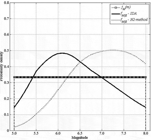
Afterwards, Eqs. (2)(2) $\begin{array}{rl}& P\left(E|M=m\right)=\int \int P\left(E|im,m,r\right)\times f_{IM|M,R}\left(im|m,r\right)dr\\ & \times f_R\left(r\right)dimdr\end{array}$(2) and (1(1) $f_{M|E}\left(m|E\right)=\frac{P\left(E|M=m\right)\times f_M(m)}{P\left(E\right)}=\frac{P\left(E|M=m\right)\times f_M(m)}{\int P\left(E|M=m\right)\times f_M(m)dm}$(1) ) can be utilized to compute the posterior distributions of magnitude (Figure 15) together with the respective uniform prior distribution. The most probable values of magnitude vary between M_w 6.10 and 7.25 for the IDA and N2-method based fragilities, respectively. Accordingly, and using Eq. (10(10) ${\mu }_{M|E}=E\left[{\mu }_{M|E,M,R}\right]\mathrm{\&}{\sigma }_{M|E}=\sqrt{E\left[{\sigma }_{M|E,M,R}^2\right]+{\sigma }_{\hspace{0.17em}}^2\left[{\mu }_{M|E,M,R}\right]}$(10) ), the expected values of magnitude range from M_w 6.39 to 6.90 with standard deviations of 0.74 and 0.68, respectively. Although these results are relatively close the 6.48 ± 0.75 obtained by Morais (2019) in a more detailed study, this discrepancy in results exemplifies the importance of the fragility functions in the magnitude estimation process.

Figure 15. Posterior distributions of magnitude using both IDA and N2-method based fragilities

7. Conclusions

The present paper focussed on the effect of modelling the seismic behaviour of historical building archetypes for the 18th c. Hungarian kingdom on fragility functions developed for the estimation of the magnitude of the 1763 Komárom earthquake. The problem is multifaceted, bounded to different types of uncertainties and raises questions on the variety of historical buildings and materials, modelling level, analysis methods and seismic record selection.

While structural archetypes for eighteenth-century Hungarian buildings were developed in previous works, the respective seismic fragilities were efficiently obtained in this paper, with the incorporation of physical uncertainties and using both nonlinear static and dynamic analyses. Hence, conclusions can be highlighted from the present study:

The fragilities obtained with the simplified DSA present lower medians but higher standard deviations, lowering resistance and increasing uncertainty of the estimates;

The fragilities resulting from IDA are more conservative than those obtained from the N2-method;

The fragility moments are generally within the ranges appearing in literature on seismic vulnerability and fragility analysis (e.g., Silva, Crowley, and Colombi 2014); although the fragilities obtained from both N2-method and IDA associate relatively low GM intensity levels to damage states in the cases of archetypes A0 to A2;

The seismic resistance is proportional to the archetype category, which may be explained by the increase in the strength parameters’ values, despite the increase in weight;

These results, consistently with Morais, Vigh, and Krähling (2018a), suggest that the growth in height, or heavier roofing with longer spans, are relatively unfavourable.

Additional research work may highlight questions that were not addressed in this paper and promote further achievements:

The modelling uncertainties arising from simplification may be studied by comparing the simplified DSA with a detailed DSA procedure using the EFM;

The 18th c. Hungarian building stock and respective strength parameters need further research in order to estimate fragilities consistent with the historical damage;

Kinematic methods may also be efficient tools to investigate, in future works, failure mechanisms reported in the historical damage descriptions;

further conclusions on the adopted simplification procedure are necessary and may be achieved by comparing the results of NSA and IDA procedures for the same equivalent-frame archetype model;

The use of Multiple Stripes Analysis together with a more detailed characterization of GM variability with a higher number of records may also be an efficient alternative for fragility analysis.

Acknowledgements

To Eng. Davide Seni and to STAdata for providing the Tremuri license. Proper acknowledgements to CAPES for funding the present research, process nº 9178-13-9. The research reported in this work was supported by the BME-Water sciences & Disaster Prevention FIKP grant of EMMI (BME FIKP-VÍZ).

Disclosure statement

No potential conflict of interest was reported by the authors.

Additional information

Funding

This work was supported by the Coordenação de Aperfeiçoamento de Pessoal de Nível (CAPES) Superior [9178-13-9]; EMMI, BME - Water sciences & Disaster Prevention FIKP grant (BME FIKP-VÍZ).

References

- Armuth, M., D. Hegyi, and Á. Sipos. 2010. Structural analysis of the baroque parish church of Zsámbék. Periodica Polytechnica Architecture 41 (2):43–47. doi:10.3311/pp.ar.2010-2.01.
- Azizi-Bondarabadi, H., N. Mendes, and P. B. Lourenço. 2019. Higher mode effects in pushover analysis of irregular masonry buildings. Journal of Earthquake Engineering 1–35. doi:10.1080/13632469.2019.1579770.
- Caporale, A., F. Parisi, D. Asprone, R. Luciano, and A. Prota. 2015. Comparative micromechanical assessment of adobe and clay brick masonry assemblages based on experimental data sets. Composite Structures 120 (1):208–20. doi:10.1016/j.compstruct.2014.09.046.
- Csicsely, Á. O. 2006. Experimental and theoretical examination of the load capacity of mud walls [in Hungarian]. PhD diss., Budapest University of Technology and Economics.
- Ditlevsen, O. 1981. Uncertainty modelling with applications to multidimensional civil engineering systems. New York: McGraw-Hill.
- Eisinger, U., R. Gutdeutsche, and C. Hammerl. 1992. Historical earthquake research - an example of interdisciplinary cooperation between geophysicists and historians. Abhandlungen Der Geologischen Bundesanstalt 48 (1):33–50.
- EN 1996- 1-1. 2005. Design of masonry structures. General rules for reinforced and unreinforced masonry structures. 1st ed. Brussels: BEL.
- EN 1998-1. 2004. Eurocode 8: Design of structures for earthquake resistance. 1st ed. Brussels: BEL.
- Fajfar, P. 1999. Capacity spectrum method based on inelastic demand spectra. Earthquake Engineering and Structural Dynamics 28 (1):979–93. doi:10.1002/(SICI)1096-9845(199909)28:9<979::AID-EQE850>3.0.CO;2-1.
- Fajfar, P. 2000. A nonlinear analysis method for performance based seismic design. Earthquake Spectra 16 (3):573–92. doi:10.1193/1.1586128.
- Freeman, S. A. 1998. Development and use of capacity spectrum method, Proceedings of the 6th US National Conference on Earthquake Engineering, Seattle, Washington, USA.
- Furtado, A., H. Rodrigues, and A. Arêde. 2015. Modelling of masonry infill walls participation in the seismic behaviour of RC buildings using OpenSEES. International Journal of Advanced Structural Engineering 7 (1):117–27. doi:10.1007/s40091-015-0086-5.
- Guerrini, G., F. Graziotti, A. Penna, and G. Magenes. 2017. Improved evaluation of inelastic displacement demands for short-period masonry structures. Earthquake Engineering & Structural Dynamics 46 (9):1411–30. doi:10.1002/eqe.v46.9.
- HAZUS-MH MR1. 2003. Multi-hazard loss estimation methodology: earthquake model HAZUS-MH MR1 technical manual. Washington DC., US: Fed. Emerg. Manag. Agency.
- Istvánfi, G. 1995. Surveys of settlements completed during the summer stages for students of architecture between 1980 and 1994 [in Hungarian]. Budapest, Hungary: BME, Inst. of Theory and Hist. of Arch.
- Kiss, B. 2017. Design and evaluation of the foundation piles of the Danube bridge of Komárom [in Hungarian], MSc diss., Budapest University of Technology and Economics.
- Krawinkler, H. 2009. Loading histories for cyclic tests in support of performance assessment of structural components, 3rd International Conference on Advances in Experimental Structural Engineering, San Francisco, pp. 10.
- Lagomarsino, S., A. Penna, A. Galasco, and S. Cattari. 2008. TREMURI: Seismic analysis program for 3D masonry buildings, User’s guide, University of Genova, Italy.
- Lagomarsino, S., A. Penna, A. Galasco, and S. Cattari. 2013. TREMURI program: An equivalent frame model for the nonlinear seismic analysis of masonry buildings. Engineering Structures 56 (1):1787–99. doi:10.1016/j.engstruct.2013.08.002.
- Lourenço, P. B., and J. A. Roque. 2006. Simplified indexes for the seismic vulnerability of ancient masonry buildings. Construction and Building Materials 20 (4):200–08. doi:10.1016/j.conbuildmat.2005.08.027.
- Lowes, L., N. Mitra, and A. Altoontash 2004. A beam-column joint model for simulating the earthquake response of reinforced concrete frames. PEER Report 2003/10 Pacific Earthq. Eng. Res. Center, College of Engineering University of California, Berkeley, US.
- Maio, R. 2013. Seismic vulnerability assessment of old building aggregates (MSc dissertation). University of Aveiro, Portugal.
- Maio, R., T. Ferreira, R. Vicente, and J. Estevão. 2016. Seismic vulnerability assessment of historical urban centres: Case study of the old city centre of Faro, Portugal. Journal of Risk Research 19 (5):551–80. doi:10.1080/13669877.2014.988285.
- Marino, S., S. Cattari, and S. Lagomarsino. 2018. Use of nonlinear static procedures for irregular URM buildings in literature and codes. In: Proc. of 16th European conference on Earthquake Engineering, Thessaloniki (GR), June 18–21.
- McKenna, F., M. H. Scott, and G. L. Fenves. 2010. Nonlinear finite element analysis software architecture using object composition. Journal of Computing in Civil Engineering 24 (1):95–107. doi:10.1061/(ASCE)CP.1943-5487.0000002.
- Morais, E. C. 2019. Estimation of the intensities of historical seismic events in moderately seismic regions, based on the damage analysis of Hungarian historical buildings. PhD diss., Budapest University of Technology and Economics.
- Morais, E. C., L. G. Vigh, and J. Krähling. 2017. Fragility estimation and comparison using IDA and simplified macro-modeling of in-plane shear in old masonry walls. Springer Proceedings in Mathematics & Statistics 181 (1):277–91.
- Morais, E. C., L. G. Vigh, and J. Krähling. 2018a. A methodology for the development of historical building archetypes for seismic performance assessment. Pollack Periodica 13 (1):203–15. doi:10.1556/606.2018.13.1.18.
- Morais, E. C., L. G. Vigh, and J. Krähling. 2018b. Influence of prior distributions and fragility assessment methods in the estimation of the magnitude of a historical seismic event. MATEC Web of Conferences 149 (1):6. doi:10.1051/matecconf/201814902038.
- MVM Paks II Ltd. 2016. Geology, geophysics, seismology, geotechnics and hydrology [in Hungarian]. Site Safety Analysis Report 2 (5):197. Accessed July 2, 2018. http://www.paks2.hu/hu/Kozerdeku/KozerdekuDokumentumok/telephely_engedelyezeDocuments.
- Nakamura, Y., H. Derakhshan, M. C. Grith, G. Magenes, and A. H. Sheikh. 2017. Applicability of nonlinear static procedures for low-rise unreinforced masonry buildings with flexible diaphragms. Engineering Structures 137:1–18. doi:10.1016/j.engstruct.2017.01.049.
- PEER. 2013. NGA-west2 ground motion prediction equations for vertical ground motions. PEER Report 2013/24, Pacific Earthquake Engineering Research Center, University of California, Berkeley.
- Pitilakis, K. 2004. Site effects. In Recent advances in earthquake geotechnical engineering and microzonation, ed. A. Ansal, 139–97. Dordrecht: Kluwer.
- Raka, E., E. Spacone, V. Sepe, and G. Camata. 2015. Advanced frame element for seismic analysis of masonry structures: Model formulation and validation. Earthquake Engineering and Structural Dynamics 44 (1):2489–506. doi:10.1002/eqe.2594.
- Rota, M., A. Penna, and G. Magenes. 2014. A framework for the seismic assessment of existing masonry buildings accounting for different sources of uncertainty. Earthquake Engineering and Structural Dynamics 43 (7):1045–66. doi:10.1002/eqe.v43.7.
- Ryu, H., J. Kim, and J. Baker. 2009. A probabilistic method for the magnitude estimation of a historical damaging earthquake using structural fragility functions. Bulletin of the Seismological Society of America 99 (2):520–37. doi:10.1785/0120080032.
- Sevieri, G., A. De Falco, M. Mori, and G. Guidetti. 2017. Model uncertainties in seismic analysis of existing masonry buildings: The equivalent-frame model within the structural element models approach. Pistoia: XVII Congress ANIDIS.
- Silva, V., H. Crowley, and M. Colombi. 2014. Fragility function manager tool. In SYNER-G: Typology definition and fragility functions for physical elements at seismic risk, geotechnical, geological and earthquake engineering, ed.. K. Pitilakis, H. Crowley, and A. M. Kaynia, 27(1): 385–402. Netherlands: Springer. https://www.springer.com/gp/book/9789400778719
- Stucchi, M., A. Rovida, A. A. Gomez Capera, P. Alexandre, T. Camelbeeck, M. B. Demircioglu, P. Gasperini, V. Kouskouna, R. M. W. Musson, M. Radulian, et al. 2013. The SHARE European earthquake catalogue (SHEEC) 1000–1899. Journal of Seismology 17 (1):523–54. doi:10.1007/s10950-012-9335-2.
- Szeidovitz, G. 1986. Earthquakes in the region of komárom. Mór and Várpalota, Geophysical Transactions 32 (1):255–74.
- Tarque, N., G. Camata, E. Spacone, H. Varum, and M. Blondet. 2014a. Non-linear dynamic analysis of a full-scaled unreinforced adobe module. Earthquake Spectra 30 (1):1643–61. doi:10.1193/022512EQS053M.
- Tarque, N., G. Camata, H. Varum, E. Spacone, and M. Blondet. 2014b. Numerical simulation of an adobe wall under in-plane loading. Earthquake and Structures 6 (1):627–46. doi:10.12989/eas.2014.6.6.627.
- Tarque, S. 2008. Seismic risk assessment of adobe dwellings. MSc diss., University of Pavia.
- Tóth, L., E. Győri, P. Mónus, and T. Zsíros. 2006. Seismic hazard in the Pannonian region. In The Adria microplate: GPS Geod., tectonics and hazards, ed. N. Pinter, 369–84. Netherlands: Springer.
- Vamvatsikos, D., and C. A. Cornell. 2002. Incremental dynamic analysis. Earthquake Engineering and Structural Dynamics 31 (1):491–514. doi:10.1002/eqe.141.
- Varga, P., G. Szeidovitz, and R. Gutdeutsch. 2001. Isoseismal map and tectonical position of the Komárom earth-quake of 1763. Acta Geodaetica Et Geophysica Hungarica 36 (1):97–108. doi:10.1556/AGeod.36.2001.1.8.
- Vicente, R. 2008. Strategies and methodologies for urban rehabilitation interventions. Vulnerability and risk assessment of the traditional building stock of the old city centre of Coimbra [in Portuguese]. PhD diss., University of Aveiro.
- Vigh, L. G., A. B. Liel, G. G. Deierlein, E. Miranda, and S. Tipping. 2014. Component model calibration for cyclic behaviour of a corrugated shear wall. Thin-Walled Structures 75 (1):53–62. doi:10.1016/j.tws.2013.10.011.
- Woessner, J., D. Laurentiu, D. Giardini, H. Crowley, F. Cotton, G. Grünthal, G. Valensise, R. Arvidsson, R. Basili, M. H. Demircioglu, et al. 2015. The 2013 European seismic hazard model: Key components and results. Bulletin of Earthquake Engineering 13 (1):3553–96. doi:10.1007/s10518-015-9795-1.
- Zimmermann, T., A. Strauss, and K. Bergmeister. 2010. Numerical investigation of historic masonry walls under normal and shear load. Construction and Building Materials 24 (1):1385–91. doi:10.1016/j.conbuildmat.2010.01.021.