The randomized method of estimating the net present value of construction projects efficiency

Abstract

The research presented in this article is a significant extension of data for company management boards, enabling them to make the right investment decisions at a very preliminary stage of investment preparation. The randomized method of estimating the net present value of construction projects efficiency allows to assess the profitability of projects under random implementation conditions. The probability and severity of disturbances are estimated. The primary initial data are randomized and the randomized probabilistic indicator of the net present value of project efficiency is calculated. Its values hovers around 1. Values larger than 1 mean that the project is profitable. Values lesser than 1 suggest stoppage of the implementation. As a supplement of the efficiency analysis the expected overall revenue, the expected total cost and the expected gross profit are calculated. All specified quantities are estimated for the actually expected and for the exceptionally notably favourable and extremely difficult implementation conditions. The method allow also estimation the risk of overall revenue in the range [1,0] and the risk of total cost in the range [0,1]. The changes of risk values in these ranges for the consecutive comparative values are presented in charts of revenue and cost risk and results table.

Highlights

1. Randomized method of estimating the net present value of construction projects efficiency unlike the others that have been published in this field of research, allows to take into account the impact of threats on the course and results of the project.

2. The rules of sustainable development can be better taken into account.

3. The method allows reliably evaluate the value and accuracy of the efficiency estimation.

Keywords:

• efficiency
• risk
• randomization
• construction project

Introduction

There are a lot of approaches to estimate efficiency of the projects. Unfortunately, all well-known methods of assessing efficiency, although they consider the time value of money, actually use deterministic data. The results obtained in this way are also deterministic (Halpin and Woodhead 1998; Cao and Song 2016; Stanitsas and Kirytopoulos 2021; Thneibat and Al-Shattarat 2021). In such cases the efficiency is usually measured as the ratio of useful result (“product”) to total outlay. But, in random conditions, the efficiency is random variable and have to be estimate taking into account an impact of random events on course and results of the project lifecycle implementation (Gorlewski 2015; Pham et al. 2021). From this point of view costs of tasks execution and revenues paid in tranches that have been initially identified should be randomized.

In statistics, the term randomization is applied to describe various random questions. For example (Nahler 2009) in order to generate a randomized process has used computer generated random numbers and tables of random numbers. Here, these numbers i.e., values of primary initial costs and revenues can be estimated. This is only approximation of real values that depend on random implementation conditions. Unfortunately, random characteristics of these quantities are unknown. So, the random characteristics have to be assigned to the primary initial data in order to characterize random costs and random revenues of the project implementation. The method can be adapted to estimate the efficiency of projects such as building constructions (Shafiei et al. 2020; Konior and Szóstak 2021), engineered constructions, industrial constructions and housing construction (Sobieraj and Metelski 2020). Generally, such construction projects are unique, as has been evidenced for example by Halpin, D. W. & Woodhead, R. W. 1998 (Kasprowicz 2011), (Ritz 1994), (De Wilde 2018). But, in all cases cost, time, quality and sustainability development are main issues of the construction projects management today (Belay and Torp 2021; Goodarzizad et al. 2021). Investors and developers analyze these conditions and evaluate profitability of the project (Porwal et al. 2020; Abdel-Hamid and Abdelhaleem 2021; Sadeh et al. 2021). This can be done using the evaluation indicators.

For example: the payback period, the net present value, the internal rate of return and the benefit cost ratio, that has been presented by (Parmenter 2015), (JASPERS 2008), (Skov 1994), et al. Generally, these indicators are reliable and well describe efficiency when the project would be implemented in the stable and balanced economic and environmental conditions. Usually, inner and outer random events can strongly affect the project implementation. Such threats can increase costs and decrease revenues of the project. The risk of the project implementation exist (Genc 2021). These problems have been studied by Cao, J., Song, W. 2016 (Braganca et al. 2010), (Radło 2015), (Kalkhoran et al. 2014), (Ward and Chapman 1995), et al.

In consequence the project deadline can be randomly delayed and the total cost can be accidentally overrun, and the project implementation quality can be probably deteriorated. Likewise, a project revenue may also change. In such case, the organization of the accomplishment, the schedule and the cost estimate should be developed taking into account random conditions of the project lifecycle implementation. From these points of view project lifecycle should be studied e.g., (Braganca et al. 2010), (Uher and Lawson 1998), et al. Unfortunately in published books and papers relevant to the project lifecycle problems predominate deterministic approach. For example: (Kasprowicz 2015) or (Kasprowicz 2011) and (Bizon-Górecka 2008).

But, because of random conditions of projects implementation, better approach is probabilistic analysis when the efficiency of the project implementation can be characterized as random variable.

Thus, the goal of the research was to develop a probabilistic method for the analysis and assessment of the net present value of the effectiveness of unstable construction projects in the conditions of the impact of significant disturbances on the course and results of their implementation.

In the article the randomized method of estimating of construction projects efficiency ex ante has been described. The value of efficiency is estimated at the stage of feasibility study on the basis of the randomized primary initial data.

Description of the method

Step 1: Comprehensive identifying of the primary initial data of the construction project implementation

The comprehensive identification of the primary initial data of the construction project implementation can be developed in the following steps:

1. Project structure, requirements and assumptions:

   • stages s, $s=1,2,\dots ,t,$ of the project life cycle;

   • subsets $A^s$ of tasks $a_i\mathrm{ }$ to be executed in the stages s: (2.1) $$A^s=\left\{a_i:i=1,2,\dots ,i^s\right\}\mathrm{ }$$(2.1)

   • the set A of all tasks $a_i$ to be executed in the project: (2.2) $$A=\bigcup _{s=1}^{s=t}{A}^s=\left\{a_i:i=1,2,\dots ,i^a\right\}\mathrm{ }$$(2.2)

   • subsets $C^s$ of costs $c_i$ of tasks $a_i$ to be executed in the stages s: (2.3) $${\mathrm{ }C}^s=\left\{c_i:i=1,2,\dots ,i^s\right\}\mathrm{ }$$(2.3)

   • the set C of costs $c_i$ of tasks $a_i$ to be executed in the project: (2.4) $$C=\bigcup _{s=1}^{s=t}{C}^s=\left\{c_i:\mathrm{i}=1,2,\dots ,i^a\right\}\mathrm{ }\mathrm{ }$$(2.4)

   • the set B of tranches $b_i$ payment of the project: (2.5) $$B=\left\{b_i:i=1,2,\dots ,i^b\right\}\mathrm{ }$$(2.5)

   • the set P of revenues $p_i$ to be paid in tranches $b_i$ of the project: (2.6) $$P=\left\{p_i:i=1,2,\dots ,i^b\right\}\mathrm{ }$$(2.6)

2. Market-based project requirements and assumptions:

   • the discount rate ${\rho }_i$ paid per year $\tau ;$

   • the discounted costs $K_i$ and the discounted revenues $D_i$ at the end of τ years for each task $a_i$ and tranche $b_i$ respectively: (2.7) $$K_i=\frac{c_i}{{\left(1+{\rho }_i\right)}^{\tau }},\mathrm{ }i=1,2,\dots ,i^a;\mathrm{ }{D}_i=\frac{p_i}{{\left(1+{\rho }_i\right)}^{\tau }},i=1,2,\dots ,i^b;\tau =0,1,2,\dots ,{\tau }^i\mathrm{ }$$(2.7)

3. Subsets ${\mathcal{K}}^s$ of discounted costs $K_i$ of tasks $a_i$ to be executed in the stages s: (2.8) $${\mathcal{K}}^s=\left\{K_i:i=1,2,\dots ,i^s\right\}\mathrm{ }$$(2.8)

   • the set κ of discounted costs $K_i$ of tasks $a_i$ to be executed in the project: (2.9) $$\mathcal{K}=\bigcup _{s=1}^{s=t}{\mathcal{K}}^s=\left\{K_i:i=1,2,\dots ,i^a\right\}$$(2.9)

   • the set D $of$ discounted revenues $d_i$ to be paid in tranches $b_i$ of the project: (2.10) $$\mathcal{D}=\left\{D_i:i=1,2,\dots ,i^b\right\}\mathrm{ }$$(2.10)

   • the primary initial discounted cost of the project: (2.11) $$K=\sum _{i=1}^{i=i^a}{K}_i\mathrm{ }$$(2.11)

   • the primary initial discounted revenue of the project: (2.12) $$D=\sum _{i=1}^{i=i^b}{D}_i\mathrm{ }\mathrm{ }$$(2.12)

4. Environmental and systemic requirements, and general assumptions of the project – in respect to primary initial data the places, the environment and systemic surroundings of the project implementation including possible threats should be identified.

In described way the primary initial data can be comprehensively identified. They constitute the starting point for further detailed analysis and initially describe implementation of the construction project lifecycle.

Step 2: Randomization of the primary initial data

Likely changes in costs and revenues can be calculated by using formulas similar to those proposed by Ding et al. (2014). In this way the degree of these changes can be measured and counted by using the random coefficients of optimism ${\underset{\_}{p}}_i$ and random coefficients of pessimism ${\overline{p}}_i.$ All coefficients should be considered separately for each task and tranche and the set of threats that can disturb tasks execution and unsettle tranches payment. All the threats cause costs $K_i\in \mathcal{K}$ and revenues $D_i\in \mathcal{D}$ to be random variables. Considering requirements, values of these quantities can be described and calculated in the following steps:

1. Identification of threats that can arise in the actually expected situation:

   • subsets $E^s,\mathrm{ }s=\overline{1,t},$ of random threats $e_{i,j},j=1,2\dots ,j^s,$ that can unsettle execution of tasks $a_i,i=1,2,\dots ,i^s,$ and can change costs $K_i\in \mathcal{K}:$ $$E^s=\left\{e_{i,j}^s:i=1,2,\dots ,i^s;j=1,2,\dots ,j^s\right\}\mathrm{ }\left(2.13\right)$$

   • the set $E$ of random threats $e_{i,j},j=1,2\dots ,j^i,$ that can unsettle execution of tasks $a_i,i=1,2,\dots ,i^a,$ and can change costs $K_i\in \mathcal{K}:$ $$E=\bigcup _{s=1}^{s=t}{E}^s=\left\{e_{i,j}:i=1,2,\dots ,i^a;j\in 1,2,\dots ,j^i\right\}\mathrm{ }\left(2.14\right)$$

   • the set $E^D$ of threats $e_{i,j},j=1,2\dots ,j^b,$ that can derail payment of tranches $b_i,i=1,2,\dots ,i^b,$ and can change revenues $D_i\in \mathcal{D}:$ $$E^D=\left\{e_{i,j}:i=1,2,\dots ,i^b;j=1,2,\dots ,j^b\right\}\mathrm{ }\left(2.15\right)$$

2. Probability and severity of costs threats:

   • $r_{i,j}\in \left[0,\mathrm{ }1\right]$ – probability of threats $e_{i,j},j=1,2\dots ,j^i,$ that can change costs $K_i\in \mathcal{K}$ of tasks $a_i\in A$ (measures the possibility of cost threats arising);

   • $c_{i,j}\in [0,\mathrm{ }1]$ – severity of threats $e_{i,j},j=1,2\dots ,j^i,$ that can change costs $K_i\in \mathcal{K}$ of tasks $a_i\in A$ (measures the strength of cost threats impact);

3. Probability and severity of revenues threats:

   • $r_{i,j}\in [0,\mathrm{ }1]$ – probability of arising of threats $e_{i,j},j=1,2\dots ,j^i,$ that can change revenues $D_i\in \mathcal{D}$ paid in tranches $b_i\in B$ (the possibility of revenues threats arising);

   • $c_{i,j}\in \left[0,\mathrm{ }1\right]$ – the severity of impact of threats $e_{i,j},j=1,2\dots ,j^i,$ that can change revenues $D_i\in \mathcal{D}$ to be paid in tranches $b_i\in B$ (the strength of revenue threats impact);

     Rules of estimating of the probability and severity of the cost and revenue threats have been presented in Tables 1 and 2.

     Below are identified which random factors affect the expected total cost, and the expected gross profit (Tables 3–6).

4. Average probability $r_i,\mathrm{ }$ and average severity $c_i$ of threats $e_{i,j}\in E,i=1,2,\dots ,i^a,j=1,2\dots ,j^i,$ that affect tasks $a_i\in A$ and costs $K_i\in \mathcal{K}:$ (2.16) $$r_i=\left(\sum _{j=1}^{j=j^i}{r}_{i,j}\right){\left(j^i\right)}^{-1};\mathrm{ }{\mathrm{ }c}_i=\left(\sum _{j=1}^{j=j^i}{c}_{i,j}\right){\left(j^i\right)}^{-1}\mathrm{ }$$(2.16)

5. Average probability $r_i,$ and average severity $c_i$ of threats $e_{i,j}\in E,i=1,2,\dots ,i^b,j=1,2\dots ,j^i$ that affect tranches $b_i\in B$ and revenues $D_i\in \mathcal{D}:$ (2.17) $$r_i=\left(\sum _{j=1}^{j=j^i}{r}_{i,j}\right){\left(j^i\right)}^{-1};\mathrm{ }{\mathrm{ }c}_i=\left(\sum _{z=1}^{j=j^i}{c}_{i,j}\right){\left(j^i\right)}^{-1}\mathrm{ }$$(2.17)

6. Impact of random threats $e_{i,j}\in E,i=1,\dots ,i^a,j=1,.,j^i,$ on tasks $a_i\in A$ and costs $K_i\in \mathcal{K}:$ (2.18) $${\underset{\_}{p}}_i=1-r_i{c}_i;\mathrm{ }{\overline{p}}_i=1-(1-r_i){(1-c}_i)\mathrm{ }$$(2.18)

   • ${\underset{\_}{p}}_i\in \left[0,1\right]$ – probabilistic coefficients of costs optimism were ${\underset{\_}{p}}_i=1$ indicate extremely favorable conditions for carrying out tasks $a_i\in A$ and possible maximum reduction of cost $K_i\in \mathcal{K}$ and ${\underset{\_}{p}}_i=0$ points an opposite case;

   • ${\overline{p}}_i\in \left[0,1\right]$ – probabilistic coefficients of costs pessimism were ${\overline{p}}_i=1$ indicate extremely difficult conditions for carrying out tasks $a_i\in A$ and possible maximum increase of costs $K_i\in \mathcal{K}$ and ${\overline{p}}_i=0$ points an opposite case;

7. Impact of random threats $e_{i,j}\in E,i=1,2,\dots ,i^b,j=1,2,.,j^i,$ on tranches $b_i\in B$ and revenues $D_i\in \mathcal{D}:$ (2.19) $${\underset{\_}{p}}_i=1-\left(1-r_i\right)\left(1-c_i\right);\mathrm{ }{\overline{p}}_i=1-r_i{c}_i\mathrm{ }$$(2.19)

   • ${\underset{\_}{p}}_i=\left[0,1\right]$ – probabilistic coefficients of revenue pessimism were ${\underset{\_}{p}}_i=1$ indicates extremely difficult conditions for carrying out tranches $b_i\in B$ payments and possible maximum decrease of revenues $D_i\in \mathcal{D}$ and ${\underset{\_}{p}}_i=0$ points an opposite case;

   • ${\overline{p}}_i=\left[0,1\right]$ – probabilistic coefficients of revenue optimism were ${\underset{\_}{p}}_i=1$ indicates extremely favorable conditions for carrying out tranches $b_i\in B$ payment and possible maximum increase of revenues $D_i\in \mathcal{D}\mathcal{ }$ and ${\overline{p}}_i=0$ points an opposite case;

Table 1. Rules of values estimating of the probability and severity of the revenues threats.

Conditions of tasks implementation	Probability of conditions ri,j	Severity of conditions ci,j	Comments
Favorable implementation conditions	[0,00 $÷$ 0,48]	[0,00 $÷$ 0,48]	Tasks $a_i\in A$ to be executed under the weaker than moderate impact of random threats ei,j;
Moderate implementation conditions	[0,49 $÷$ 0,51]	[0,49 $÷$ 0,51]	Tasks $a_i\in A$ to be executed under the impact of default average random threats ei,j
Difficult implementation conditions	[0,52 $÷$ 1,00]	[0,52 $÷$ 1,00]	Tasks $a_i\in A$ to be executed under the stronger than moderate impact of random threats ei,j

Table 2. Rules of values estimating of the probability and severity of the revenues threats.

Conditions of tasks implementation	Probability of conditions ri,j	Severity of conditions ci,j	Comments
Favorable implementation conditions	[0,00 $÷$ 0,48]	[0,00 $÷$ 0,48]	Tranches $b_i\in B$ to be paid under the weaker than moderate impact of random threats ei,j
Moderate implementation conditions	[0,49 $÷$ 0,51]	[0,49 $÷$ 0,51]	Tranches $b_i\in B$ to be paid under the impact of average default random threats ei,j
Difficult implementation conditions	[0,52 $÷$ 1,00]	[0,52 $÷$ 1,00]	Tranches $b_i\in B$ to be paid under stronger than moderate impact of random threats ei,j

Table 3. Endangerment of costs e_i,j.

Stage s	Number of endangerment ej	Specification
F1 ex ante	1	Modification of the terms of financing operational analysis
	2	System of communication – mistakenly referred to the scope of the reconstruction
	3	Technical conditions of connection to the utilities, e.g., water supply and sewerage, energy, communication technology, gas etc., significantly different from the assumptions
	4	Reconstruction of the collision of the technical infrastructure in a much expanded, unpredicted range
	5	Analysis of the absorbency of the terrain incompatible with possible to obtain of development
F2 ex ante	1	Collapse of the design office
	2	Modification of the rules of law or delivery terms
	3	Collapse of the housing sales market
F3 ex ante	1	Change in prices of goods and services.
	2	Collapse of the services market of construction.
	3	Collapse of the project’s general contractor.
F4 ex ante	1	Disclosure of hidden defects and removal them within the product warranty or warranty for physical defects
	2	Cost of maintenance of unsold homes (apartments, usable premise, parking lots etc. significantly exceeding budgetary assumptions)
	3	Cost of the construction completion – beyond the contract with the project’s general contractor

Table 4. Endangerment of revenues e_i,j.

Stage	Number of endangerment ej	Specification
D	1	Price decline of apartments
	2	Decline (slackening) in sale of apartments
	3	Tighter credit policies by banks (financial restriction of investment)

Table 5. Probability r_i,j of the impact of endangerment on costs and revenues.

Level number	Description	Level	ri,j
1	Much smaller than common (extremely small)	Level 1	0,00 − 0,24
2	Slightly lesser than common (little)	Level 2	0,25 − 0,49
3	Common probability of endangerment appearance	Level 3	0,50
4	Slightly greater than common (high)	Level 4	0,51 − 0,74
5	Much greater than common (extremely high)	Level 5	0,75 − 1,00

Table 6. Severity c_i,j/d_i,j of the impact of endangerment on costs (c_i,j) and revenues (d_i,j).

Level number	Description	Level	ci,j / di,j
1	Much lesser than ordinary	Level 1	0,00 − 0,24
2	Slightly lesser than ordinary	Level 2	0,25 − 0,49
3	An ordinary impact of endangerment on the task implementation costs/revenue	Level 3	0,50
4	Slightly grater than ordinary	Level 4	0,51 − 0,74
5	Much greater than ordinary	Level 5	0,75 − 1,00

In described way, the primary initial data can be fully randomized adequately to the projected random threats of costs and revenues. Randomization can be done for actually expected as well as exceptionally possible notably favorable and extremely difficult implementation conditions.

Step 4: Randomized costs of tasks and revenues of tranches

In this case, as it has been proved by Hajdu and Bokor (2016), the inaccuracy of the PERT three-point estimation has greater effect on the distribution of the project duration than the type of activity duration distribution applied. So, the most probable values of particular tasks cost and relevant tranches of revenue should be estimated by experts based on thorough analysis of project lifecycle implementation as well as the way of tasks execution and the method of tranches payment. Next, taking additionally into account an impact of random threats on a way of tasks execution and a method of tranches payment, bottom boundary values and upper boundary values of these variables can be estimated. Suitable bottom boundary values can be calculated with respect to the most probably values by means of random coefficients of cost optimism and random coefficients of revenue optimism. Appropriate upper boundary values can be calculated with respect to the most probably values by means of random coefficients of cost pessimism and random coefficients of revenue pessimism. Using three estimated values – bottom boundary, the most probable and upper boundary – for random variables of costs and random variables of revenues, according to simplified PERT-beta formulas, expected values of these variables can be calculated. In described way the primary initial data can be transformed into the randomized computational data and credibly describe the future construction project implementation under the impact of random threats. It can be done as follows:

1. Verification tasks costs and tranches of revenues according to the actually expected market-based conditions as well as project requirements and assumptions:

   • scrutinizing and transforming costs $K_i$ into the most probable values of costs ${\widehat{K}}_i$ and establishing sets ${\widehat{K}}^s$ and $\widehat{K}:$ (2.20) $${\widehat{K}}^s=\left\{{\widehat{K}}_i:i=1,2,\dots ,i^s\right\}\text{ for }s=1,2,\dots ,t\mathrm{ }$$(2.20) (2.21) $$\widehat{K}={\mathrm{U}}_{s=1}^{s=t}{\widehat{K}}^s=\left\{{\widehat{K}}_i:i=1,2,\dots ,i^a\right\}\mathrm{ }\mathrm{ }$$(2.21)

   • scrutinizing and transforming revenues $D_i$ into the most probable values of revenues $D_i$ and establishing a set $\widehat{D}$ (2.22) $$\widehat{D}\mathrm{ }=\left\{{\widehat{D}}_i:i=1,2,\dots ,i^b\right\}\mathrm{ }$$(2.22)

   • testing and estimating the computational discount rate $\rho$ paid per year $\tau ;$

2. Likely costs of the tasks execution in the random conditions of project implementation:

   • optimistic costs ${\underset{\_}{K}}_i$ of tasks $a_i,i=1,2,\dots ,i^a$ – bottom boundary values: (2.23) $${\underset{\_}{K}}_i={\widehat{K}}_i-{\underset{\_}{p}}_i{\widehat{K}}_i\mathrm{ }$$(2.23)

   • pessimistic costs ${\overline{K}}_i$ of tasks $a_i,i=1,2,\dots ,i^a$ – upper boundary values: (2.24) $${\overline{K}}_i={\widehat{K}}_i+{\overline{p}}_i{\widehat{K}}_i\mathrm{ }$$(2.24)

   • expected values $E\left[K_i\right]\mathrm{ }$ of costs $K_i$ of tasks $a_i,i=1,2,\dots ,i^a:$ (2.25) $$E\left[K_i\right]=\frac{{\underset{\_}{K}}_i+{4\widehat{K}}_i+{\overline{K}}_i}{6}\mathrm{ }$$(2.25)

   • variances ${\sigma }^2\left[K_i\right]$ of costs $K_i$ of tasks $a_i,\mathrm{ }i=1,2,\dots ,i^a:$ (2.26) $${\sigma }^2\left[K_i\right]={\left(\frac{{\overline{K}}_i-{\underset{\_}{K}}_i}{6}\right)}^2\mathrm{ }$$(2.26)

3. Likely revenues paid in tranches in the random conditions of project implementation:

   • pessimistic revenues ${\underset{\_}{D}}_i$ paid in tranches $b_i,$ $i=1,2,\dots ,i^b$ – bottom boundary values: (2.27) $${\underset{\_}{D}}_i={\widehat{D}}_i-{\underset{\_}{p}}_i{\widehat{D}}_i\mathrm{ }$$(2.27)

   • optimistic revenues ${\overline{D}}_i$ paid in tranches $b_i,$ $i=1,2,\dots ,i^b$ – upper boundary values: (2.28) $${\overline{D}}_i={\widehat{D}}_i+{\overline{p}}_i{\widehat{D}}_i\mathrm{ }$$(2.28)

   • expected values $E\left[D_i\right]$ of revenues $D_i$ paid in tranches $b_i,$ $i=1,2,\dots ,i^b:$ (2.29) $$E\left[D_i\right]=\frac{{\underset{\_}{D}}_i+{4\widehat{D}}_i+{\overline{D}}_i}{6}\mathrm{ }$$(2.29)

   • variances ${\sigma }^2\left[D_i\right]$ of revenues $D_i$ paid in tranches $b_i,$ $i=1,2,\dots ,i^b:$ (2.30) $${\sigma }^2\left[D_i\right]={\left(\frac{{\overline{D}}_i-{\underset{\_}{D}}_i}{6}\right)}^2\mathrm{ }$$(2.30)

Based on the estimated expected values of particular costs and individual revenues, the total cost and overall revenue of the project can be estimated

Step 5: Randomized total cost and overall revenue of the construction project

Based on the randomized data, the expected value of total project cost can be calculated by using the formulas:

1. Probabilistic characteristics of the project total cost:

   • the expected value $E\left[K\right]$ of total cost of the project: (2.31) $$E\left[K\right]=\sum _{i=1}^{i=i^a}E\left[K_i\right]\mathrm{ }$$(2.31)

   • the variance ${\sigma }^2\left[K\right]$ of total cost of the project: (2.32) $${\sigma }^2=\sum _{i=1}^{i^a}{\sigma }^2\left[K_i\right]\mathrm{ }$$(2.32)

     As regards revenue, taking into account rules and the way of tranches payment, one can confirm that individual tranches are paid relatively independently of each other. Tranches are physically relatively independent of each other. So, random variables of revenues describing revenues of individual tranches payment are independent and are uncorrelated. These variables take nonzero values. Thus, the expected value of overall project revenue can be calculated as the sum of expected values of random variables of revenues paid in tranches. In this way, based on the randomized data the expected value of overall project revenue can be calculated by using the formulas:

2. Probabilistic characteristics of the project overall revenue:

   • the expected value $E\left[D\right]$ of overall revenue of the project: (2.33) $$E\left[D\right]=\sum _{i=1}^{i=i^b}E\left[D_i\right]\mathrm{ }$$(2.33)

   • the variance ${\sigma }^2\left[D\right]$ of overall revenue of the project: (2.34) $${\sigma }^2\left[D\right]=\sum _{i=1}^{i=i^b}{\sigma }^2\left[D_i\right]\mathrm{ }$$(2.34)

     The expected total cost $E\left[K\right]$ and the expected overall revenue $E\left[D\right]$ of the project describe only one case of the project implementation. It is interesting the range of probable changings of these values. These variations can be measured by using coefficients of the risk of total cost p(k) and the risk of overall revenue p(d). Values of these quantities can be calculated assuming Student’s t-distribution functions of the random variable of total cost K and the random variable of overall revenue D by using formulas:

3. Cost risk (contingency) p(k) of total cost of the project: (2.35) $$p\left(k\right)=P\left[E\left(K\right)\le k\right]=Z\left[\frac{k-E\left(K\right)}{\sqrt{{\sigma }^2\left(K\right)}}\right]\mathrm{ }$$(2.35)

   $k$ – comparative values of total cost.

4. Revenue risk (contingency) p(d) of overall revenue of the project: (2.36) $$p\left(d\right)=P\left[E\left(D\right)\ge d\right]=1-P\left[E\left(D\right)\le d\right]=1-Z\left[\frac{d-E\left(D\right)}{\sqrt{{\sigma }^2\left(D\right)}}\right]\mathrm{ }$$(2.36)

   $d$ – comparative values of overall revenue.

In proposed approach, a measure of risk of total cost $p(k)\in \left[0,1\right]$ is the probability that the expected value of project total cost $E\left[K\right]$ is lesser than comparative amount k. The risk $p\left(k\right)=0$ is indicated by a minimum cost $\underset{\_}{k}$ and means that the project expected total cost $E\left[K\right]$ should not be lesser than this value. The risk $p\left(k\right)=1$ is indicated by a maximum cost $\overline{k}$ and means that the project expected total cost $E\left[K\right]$ should be lesser than this value.

A measure of risk of overall revenue $p(d)\in [1,\mathrm{ }0]$ is the probability that the expected value of the project overall revenue $E\left[D\right]$ exceeds a comparative amount d. The risk $p\left(k\right)=1$ is indicated by minimum revenue $\underset{\_}{d}$ and means that project expected overall revenue $E\left[D\right]$ is greater than this value. The risk $p\left(k\right)=0$ is indicated by maximum revenue $\overline{d}$ and means that the project expected overall revenue $E\left[D\right]$ should not be greater than this value. The risk of project total cost and the risk of project overall revenue can be shown in the risk charts.

Sample risk chart of the analyzed investment is presented below (Figure 1).

Figure 1. Risk charts of the total cost and overall revenue of the example investment.

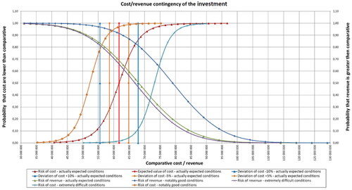
The graph of the risk of total cost and total revenues from the implementation of housing investments is built in the following layout: the axis of cut off are the values for costs and revenues, respectively. The ordinate axis in the left-hand system are the values of the probability that the corresponding costs will be lower than the comparative ones, right -hand, that the values of the probability of revenues will be higher than the comparative ones. This arrangement allows you to combine all cost and revenue curves on one chart. The expected values of costs and revenues correspond to an order of 0.5. Above and below the ordinate of 0.5 – we get a reading of the probability value and adding costs and revenues to them. In such a system, the slope of the curves allows you to assess the speed of changes in the probability of threats depending on possible changes in costs and revenues (Table 7).

Table 7. Comparison the “behaviour” of the classical NPV indices under probabilistic conditions with the “classic” results.

	Conditions
	Deterministic	Probabilistic
Description	Classic data	Randomized data	As-built data
Market-based conditions of property sales	Extremely favorable	Difficult	Difficult
Market-based conditions for labor, works and construction products	Average	Average	Average
Overall revenue (PLN)	90 300 000	68 427 404	66 990 000
Total cost (PLN)	67 800 000	61 852 247	60 939 000
The net present value of the residential housing development efficiency	1,33	1,11	1,10
Standard deviation of the net present value of randomized efficiency		0,17
Gross profit (PLN)	22 500 000	6 575 157	6 051 000
Exceptionally possible project implementation conditions	Notably favorable	Extremely difficult
Overall revenue (PLN)	87 615 830	62 582 735
Total cost (PLN)	52 294 092	73 211 729
The net present value of randomized efficiency of the residential housing development ($\mathit{NPE}$)	1,68	0,85
Gross profit (PLN)	35 321 737	−10 628 994

The analysis of the above table is a significant extension of data for company management boards, enabling them to make the right investment decisions at a very preliminary stage of investment preparation. It is estimation of probabilistic revenues and costs, which are processed using the method into subsequent probabilistic data leading to final results allowing to determine the ranges of costs and revenues with a specific probability distribution.

Results

The net present value of the construction project efficiency means here a probabilistic indicator that determines the gainfulness degree of project implemented under random conditions, when likely random threats can influence on the really revenue obtained and cost incurred. This is a random variable that is equal a quotient of random variable of project overall revenue and random variable of project total cost. Probability density function of such random quotient variable is very complicated and practically impossible to define. But, as it has been previously proved, the random variable of project overall revenue, that represent sum of revenues payment in tranches, and the random variable of project total cost, that represent sum costs of tasks execution, are independent, uncorrelated and take positive and nonzero values. Therefore, it is proposed to estimate the net present value of the construction project efficiency as the ratio of the expected value of project overall revenue to the expected value of project total cost. This is reasonable for the quotient of two random variables that are independent, uncorrelated and take positive and nonzero values. Taking under consideration researches that has been presented by Frishman (1971), Benjamin and Cornell (2014), calculations of these quantities can be done as follows:

1. The net present value of the randomized efficiency of the construction project: (3.1) $$\mathit{NPE}=E\left[\frac{D}{K}\right]=\frac{E\left[D\right]}{E\left[K\right]}\text{ provided that }E\left(K\right)\ne 0\mathrm{ }$$(3.1)

2. Variance of efficiency: (3.2) $$\mathit{Var}\left(\mathit{NPE}\right)=\mathit{Var}\left[\frac{D}{K}\right]=\frac{\mathit{Var}\left(D\right)\mathrm{*}{\left[E\left(K\right)\right]}^2-\mathit{Var}\left(K\right)\mathrm{*}{\left[E\left(D\right)\right]}^2}{{\left[E\left(K\right)\right]}^2\mathrm{*}\left\{\mathit{Var}\left(K\right)+{\left[E\{K\right]}^2\right\}}\mathrm{ }$$(3.2)

3. Standard deviation of efficiency: (3.3) $$\left(\mathit{RPE}\right)=\sqrt{{\sigma }^2\left(\mathit{RPE}\right)}\mathrm{ }$$(3.3)

4. Expected gross profit: (3.4) $$E\left[Z\right]=E\left[D-K\right]=E\left[D\right]-E\left[K\right]\mathrm{ }$$(3.4)

Using this efficiency indicator the gainfulness of the project implementation can be easy and reliable evaluated. The values of the indicator hovers around 1. Values greater than 1 mean that the project can be beneficial and is worth to implement. The values lesser than 1 can be the basis for stoppage of the project implementation. Of course, finally, which value of indicator can be evaluated as enough profitable depend directly on decision-maker.

The method was used to investigate three building investments, which were marked and named: Investment 1, Investment 2, Investment 3.

Investment 1 is a construction project in the form of a multi-family housing estate. During the cycle of implementation of the construction project, two key events took place. The first is the collapse of the construction market, the fall in housing prices and the general crisis on the construction services market, the second is the declaration of bankruptcy by the general contractor in the final phase of the investment. The investment was analyzed ex post. The investor assumed an efficiency of 1.33 without anticipating the risks that arose. The Method used, taking into account the risks involved, calculated the efficiency at the level of 1.10 – this was also confirmed by the final settlement of the investment.

Investment 2 is a construction project, similar to Investment 1, in terms of: size, location, standard of investment performance. It was implemented in a period of very good economic situation on the housing construction market, particularly good conditions were adopted. The investor assumed an ex-ante efficiency of 1.24. The method calculated the efficiency at the level of 1.23. The final settlement of the investment confirmed the effectiveness of 1.23.

Investment 3 is a small, one-stage investment of multi-family housing. The investor assumed initial data enabling the efficiency to be achieved at the level of 1.22. The method was used before the start of the investment, assuming moderate conditions of the project, the final results obtained as a result of the calculations calculated the efficiency at the level of 1.17. The final settlement of the investment confirmed the efficiency at the level of 1.17.

The initial budget specified in the study phase contains the planned efficiency. Residential investments of the development market with an average size of 200-300 apartments assume an efficiency value of 1.20 − 1.35. An investment whose initial budget determines the efficiency at the level of less than 1.20 is an investment of increased risk and threatens with loss of stability. The developed method provides additional data: about risk, theoretically possible, cost and revenue limit values and the dynamics of changes in the probability of threats depending on possible changes in costs and revenues The combined analysis of the preliminary budget, together with the results obtained after applying the method, give the management boards of development companies a more complete picture and sufficient data to make a decision on the continuation of the construction project or its abandonment, only in exceptional cases of suspension Such decisions are made at the latest before the design studies are commissioned.

Discussion

The net present value of the construction project efficiency in random implementation conditions is a probabilistic indicator of construction projects profitability. The acceptable value of this indicator should be greater than 1. It can be the basis for making decision to suspend or continue the preparation and implementation of the construction project. This indicator can be estimated reliably, reasonably and understandably and is convenient and simple to apply. It well measures the degree of the net present value of the project efficiency in random implementation conditions. It is easy-to-interpret of the project profitability. Complete with analysis of a risk of total cost and a risk of overall revenue this is comprehensive evaluation of the project viability. Thanks to that, the method can be easily used in practice. The good and convenient computer program to calculation of efficiency indicator can be prepared on the basis of a common program with spreadsheets. The program, after inputting of the primary initial data, the probabilities and severities of random threats of costs and revenues, should automatically generate the net present value of the randomized efficiency of the construction project and all other quantities. Moreover, the program should enable to develop risk charts of overall revenue $E\left[D\right]$ for consecutive comparative revenues d in the range of values $\left[\mathrm{ }\underset{\_}{d},\overline{d}\mathrm{ }\right]$ and risk values [1, 0]. The program should also enable to develop risk charts of total cost $E\left[K\right]$ for consecutive comparative costs k in the range of values $\left[\mathrm{ }\underset{\_}{k},\overline{k}\mathrm{ }\right]$ and risk values [0, 1]. The program is very simple and can be easily adjusted to individual use.

It is possible to use the program in collaboration in further research.

In conclusion, it worth to point out the possible improvement and further research of the presented method. At present, the study has been launched concerns the possibility, needs and feasibility applying methods of artificial intelligence in the process of identifying, analyzing and estimating the net present value of construction projects having regard to an impact of threats on implementation course and results of projects. In particular, the study should concern the identification of the primary initial data, the definition of a set of threats for costs and revenues, the estimation of the probability and severity of threats and the risk analysis of total cost and overall revenue. From this point of view, it would be useful to create and apply an appropriate set of "big data" comprehensively characterizing the project implementation. Based on the results of the preliminary study of these problems one can confirm that this is possible and would bring the method closer to the needs of practice.

Disclosure statement

(i) Nothing to Disclose

No potential conflict of interest was reported by the authors.

(ii) Proprietary Data

All data used in the article are based on official stock exchange announcements of Polish development companies. Further approvals, developments and detailed analyses are the result of the knowledge and experience of the authors. No sensitive data of development companies were used in the study, nor was the trade secret compromised.

(iii) Other Cases

There is no information in the article that may conflict with financial, moral or any other potential interests of anybody.

References

- Abdel-Hamid M, Abdelhaleem HM. 2021. Project cost control using five dimensions building information modelling. Int J Construct Manage. 21:1–10. https://doi.org/10.1080/15623599.2021.1880313.
- Belay AM, Torp O. 2021. Construction cost performance under quality-gated framework: the cases of Norwegian road constructions. Int J Construct Manage. 21:1–14. https://doi.org/10.1080/15623599.2021.1949670.
- Benjamin JR, Cornell CA. 2014. Probability, statistics, and decision for civil engineers. Manufactured in the United States by Courier Corporation. Mineola, NY: Dover Publications.
- Bizon-Górecka J. 2008. O zarządzaniu projektami inwestycyjno-budowlanymi z uwzględnieniem czynników ryzyka. Przegląd Budowlany. 79:42–46.
- Braganca L, Kokkari H, Veljkovic M, Borg RP. 2010. Sustainable Construction. A Life Cycle Approach in Engineering. International Training School. Malta: Faculty for the Built Environment, University of Malta. ISBN/ISSN: 978-99932-0-918-8.
- Cao J, Song W. 2016. Risk assessment of co-creating value with customers: A rough group analytic network process approach. Expert Syst Appl. 55:145–156.
- De Wilde P. 2018. Building performance analysis. Hoboken, NJ: John Wiley and Sons Ltd.
- Ding L, Zhou Y, Akinci B. 2014. Building Information Modeling (BIM) application framework: The process of expanding from 3D to computable nD. Autom Constr. 46:82.
- Frishman F. 1971. On the arithmetic means and variances of products and ratios of random variables. Durham (NC): Army Research Office. www.dtic.mil/dtic/tr/fulltext/u2/785623.pdf.
- Genc O. 2021. Identifying principal risk factors in Turkish construction sector according to their probability of occurrences: a relative importance index (RII) and exploratory factor analysis (EFA) approach. Int J Construct Manage. 21:1–9. https://doi.org/10.1080/15623599.2021.1946901.
- Goodarzizad P, Golafshani EM, Arashpour M. 2021. Predicting the construction labour productivity using artificial neural network and grasshopper optimisation algorithm. Int J Construct Manage. 21:1–17. https://doi.org/10.1080/15623599.2021.1927363.
- Gorlewski B. 2015. Project effectiveness evaluation. Warsaw: Warsaw School of Economics.
- Hajdu M, Bokor O. 2016. Sensitivity analysis in PERT networks: Does activity duration distribution matter? Autom Constr. 65:1–8. Vol
- Halpin DW, Woodhead RW. 1998. Construction management. 2nd ed. Canada: John Wiley & Sons Inc.
- JASPERS. 2008. Blue Book. Road infrastructure. Joint assistance to support projects in European regions. Warsaw: Ministry of Infrastructure.
- Kalkhoran SHA, Liravi G, Rezagholi F. 2014. Risk management in construction projects. IJETT. 10(3):133–138.
- Kasprowicz T. 2011. Analiza ryzyka przedsięwzięć budowlanych. Budownictwo i Inżynieria Środowiska, Zeszyt. 58(3/2011/III):233–240.
- Kasprowicz T. 2015. Inżynieria przedsięwzięć budowlanych. In: Kasprowicz T, (red.) Inżynieria Przedsięwzięć Budowlanych, rekomendowane metody i techniki, wyd. PAN KIWiL, Sekcja. Warszawa: IPB; p. 10–20.
- Konior J, Szóstak M. 2021. Course of planned, actual and earned cost curves of diverse construction investments. Int J Construct Manage. 21:1–12. https://doi.org/10.1080/15623599.2021.1942769.
- Nahler G. 2009. Randomization. In: Dictionary of pharmaceutical medicine. Vienna: Springer; p. 154–155.
- Parmenter D. 2015. Key performance indicators: Developing, implementing, and using winning KPIs. Copyright by David Parmenter. Hoboken, NJ: John Wiley & Sons, Inc.
- Pham TQD, Le-Hong T, Tran XV. 2021. Efficient estimation and optimization of building costs using machine learning. Int J Construct Manage. 21:1–13. https://doi.org/10.1080/15623599.2021.1943630.
- Porwal A, Parsamehr M, Szostopal D, Ruparathna R, Hewage K. 2020. The integration of building information modeling (BIM) and system dynamic modeling to minimize construction waste generation from change orders. Int J Construct Manage. 20:1–20. https://doi.org/10.1080/15623599.2020.1854930.
- Radło MJ. 2015. Risk management in integrated management systems. Warsaw: Warsaw School of Economics.
- Ritz G. 1994. Total construction project management. New York City: McGraw Hill Education.
- Sadeh H, Mirarchi C, Shahbodaghlou F, Pavan A. 2021. BIM feasibility for small and medium-sized contractors and subcontractors. Int J Construct Manage. 21:1–10. https://doi.org/10.1080/15623599.2021.1947446.
- Shafiei I, Eshtehardian E, Nasirzadeh F, Arabi S. 2020. Dynamic modeling to reduce the cost of quality in construction projects. Int J Construct Manage. 20:1–14. https://doi.org/10.1080/15623599.2020.1845425.
- Skov NW. 1994. Finance & management. In: The American Model Applied to Polish Private Enterprise. Warsaw: PRET.
- Sobieraj J, Metelski D. 2020. Identification of the key investment project management factors in the housing construction sector in Poland. Int J Construct Manage. 20:1–12. https://doi.org/10.1080/15623599.2020.1844855.
- Stanitsas M, Kirytopoulos K. 2021. Investigating the significance of sustainability indicators for promoting sustainable construction project management. Int J Construct Manage. 21:1–26. https://doi.org/10.1080/15623599.2021.1887718.
- Thneibat MM, Al-Shattarat B. 2021. Critical success factors for value management techniques in construction projects: case in Jordan. Int J Construct Manage. 21:1–22. https://doi.org/10.1080/15623599.2021.1908933.
- Uher TE, Lawson W. 1998. Sustainable development in construction. Proceedings CIB World Building Congress, Gaevle, Sweden, 7–12 June 1998.
- Ward SC, Chapman CB. 1995. Risk-management perspective on the project lifecycle. Int J Project Manage. 13/3:145–149.