Multi-driver ensemble to evaluate the water utility business interruption cost induced by hydrological drought risk scenarios in Brazil

ABSTRACT

Climate change and increasing water demand in urban environments necessitate planning water utility companies’ finances. Traditionally, methods to estimate the direct water utility business interruption costs (WUBIC) caused by droughts have not been clearly established. We propose a multi-driver assessment method. We project the water yield using a hydrological model driven by regional climate models under radiative forcing scenarios. We project water demand under stationary and non-stationary conditions to estimate drought severity and duration, which are linked with pricing policies recently adopted by the Sao Paulo Water Utility Company. The results showed water insecurity. The non-stationary trend imposed larger differences in the drought resilience financial gap, suggesting that the uncertainties of WUBIC derived from demand and climate models are greater than those associated with radiative forcing scenarios. As populations increase, proactively controlling demand is recommended to avoid or minimize reactive policy changes during future drought events, repeating recent financial impacts.

KEYWORDS:

• Business interruption cost
• water utility company
• hydrological droughts
• water security
• urban water
• climate change

1. Introduction

Water utility company business interruption costs (WUBIC) refers to the financial losses a company suffers when its operations are disrupted, which is characterized by global and regional trends. On the one hand, climate change, population growth, the non-stationary nature of climate extremes, and uncontrolled human development make society more claimant on water (Montanari et al. 2013). On the other hand, the ever larger mobilization of water and the use of new supply sources for growing demands is already seen as an untenable idea (Falkenmark and Lannerstad 2004). Such pressure on water resources inhibits the socioeconomic development of communities (Laaha et al. 2016; Wada et al. 2013; Van Loon et al. 2016a; Lloyd-hughes 2013).

Droughts have a great impact, mainly because of their broad geographic coverage, time duration, and lasting damage (Bressers, Bressers, and Corinne 2016; Smakhtin and Schipper 2008; Van Lanen et al. 2013; Bucheli, Dalhaus, and Finger 2020). Furthermore, more severe and prolonged droughts are expected in the future, leading to greater economic consequences, environmental degradation, and loss of human lives (Shi et al. 2015; Stahl et al. 2016; Freire-González, Decker, and Hall 2017; Balbus 2017; Asadieh and Krakauer 2017; Prudhomme et al. 2014; Berman et al. 2013; Touma et al. 2015; Ault 2020; Ali et al. 2021). Therefore, it is essential to create adequate risk perception, aiming to reduce vulnerability, mitigate the impacts, and build a more resilient and cautious community to deal with droughts (Mishra and Singh 2010; Nam et al. 2015; S Bachmair et al. 2016; Liu et al. 2021).

Hydrological drought is defined as a negative anomaly in surface and subsurface water levels that can extend over a long time period (Van Loon 2015; Wanders, Van Loon, and Van Lanen 2017; Mishra and Singh 2010). These negative anomalies associated with excessive demand can cause disruptions in the water supply systems (Mehran, Mazdiyasni, and Aghakouchak 2015; Van Loon, Van Loon et al. 2016b; Wanders and Wada 2015). One way water utility companies traditionally prepare against such anomalies is through supply augmentation (Sahin et al. 2018). To reduce vulnerability, rethinking the way forward is required, given the scarcity of new sources (Wanders and Wada 2015).

In Brazil, from 2013 to 2015, the population of the São Paulo Metropolitan Region (SPMR) experienced the most acute water crisis in its history (Nobre and Marengo 2016; Taffarello et al. 2016; Coutinho, Kraenkel, and Prado 2015). The 2013–2015 crisis caused a business interruption of nearly 60,000 water-dependent productive institutions according to the Sao Paulo Federation of Industries (FIESP), representing almost 60% of the state’s industrial GDP (Marengo et al. 2015). Among the companies most affected was the Sao Paulo State Water Utility Company (SABESP). The total economic damage attributed to the drought in 2014 was estimated to be between 3 and 5 billion USD (Nobre et al. 2016), including large losses to agriculture, but SABESP alone saw an income drop of more than 200 million USD (see supplementary material). Water demand management has proven to be a viable alternative to support water security in urban environments (Sahin et al. 2018). Based on this, SABESP has been implementing price mechanisms to discourage water demand during deficit periods. However, these measures affected the company’s main business, leading to an important liquid net income reduction compared to previous years (around 65%, see Supplementary Material), a major financial crisis in the company (SABESP, GESP 2016; SABESP 2017c). Therefore, this study proposes an approach to estimate the WUBIC to reduce financial vulnerability by integrating future climate uncertainty and growing water demand.

The definitions of drought losses or drought costs are diverse and not fully agreed upon (Freire-González, Decker, and Hall 2017; Meyer et al. 2013; Logar and van den Bergh 2012; Ault 2020; Liu et al. 2021). Drought costs can be separated across direct, indirect, and non-market costs (Logar and van den Bergh 2012), from which business interruption costs as primary tangible costs can be further differentiated (Meyer et al. 2013), although not configured as ‘due to direct physical contact’. Despite the diverse range of methods found in the literature, several are for non-tangible or indirect methods, specific for the agricultural sector, or economy-wide oriented (i.e. fit to a broader scale application), which would incur less precise results in our case. Regarding the impact of reduced water availability on water utilities (the WUBIC) several approaches seem adequate, such as market valuation techniques or ex-post evaluations (i.e. comparing changes in GDP or changes in price between affected and unaffected years).

We tested our approach using a semi-distributed hydrological model driven by the outputs of a regional climate model and projected water demand pressure based on population growth. We characterize the water deficit through the severity–duration–frequency approach relating water cost and the storage system state throughout the running scenarios.

2. Water crisis contextualization and study area

Changes in rainfall trends and temperature extremes in southeast Brazil, together with user growth, progressively reveal SPMR water vulnerability (Chou et al. 2014a; Zuffo 2015; Buckeridge M and Ribeiro 2018; Ussami and Guilhoto 2018). Severe water shortages were recorded in the SPMR, driven by precipitation anomalies in 1953–1954, 1962–1963, 1984, and 2001 (Cavalcanti and Kousky 2001; Buckeridge M and Ribeiro 2018). The 1962–1963 event apparently motivated the construction of the main water source of SPMR, the Cantareira Water Supply System (CWSS) (Nobre et al. 2016). The system designed to supply the increasing water demand of SPMR began its partial operation in 1974, and its construction was completed in 1981 with a 30-year permit to transfer up to 35 m³/s, an amount that has been periodically evaluated since the last water crisis (Mohor and Mendiondo 2017). The CWSS is currently administered by SABESP, the main operator of the water network in the SPMR, and the government of Sao Paulo state is its main shareholder.

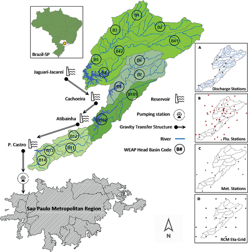
The CWSS is located in Southeast Brazil between the states of Sao Paulo and Minas Gerais. The rainy season in the CWSS generally begins at the end of September and ends in March. During this period, an average of 72% of the annual rainfall accumulated (Marengo et al. 2015). In hydrological terms, the 2265 km² of drainage area, has historically generated an annual mean tributary discharge of 38.74 m³/s, regulated by storage and transfer structures. The system is composed of four interconnected dams with a useful total storage volume of 988.8 hm³, arranged to transfer water from the Piracicaba River Basin to the Upper Tietê Basin (Figure 1). The system was configured to supply approximately 11 million people in the SPMR prior to the 2013–2015 crisis (Agencia das Bacias PCJ, Comitês PCJ 2016; Nobre and Marengo 2016; De Andrade 2016; Marengo et al. 2015; Nobre et al. 2016; PCJ/Comitês 2006).

Figure 1. System structure composition and catchment areas of the ‘cantareira water supply system’. Jaguarí-Jacareí (B1, B2, B3, B41, B42, B5 and B8), Cachoeira (B6, B7 and B9), Atibainha (B101 and B102), and Paiva Castro (B11, B12; B13 and B14). panel A: discharge gauge stations; panel B: rainfall gauge stations; panel C: meteorological gauge stations and panel D: centroid of the eta-INPE (RCM) grid.

During the 2013–2015 crisis, SABESP undertook reactive measures to control the consumption in the SPMR (Marengo et al. 2015) such as: Extraordinary increases of water tariff prices; programmed water cut-offs; economic bonuses and penalties to ration water consumption; network pressure reduction; water use from ‘dead storage’ (when storage level is below extraction by gravity and needs to be pumped); social awareness campaigns to inform people about shortages; and water distributed by tankers in the most critical areas to provide the human Basic Water Requirement (BWR) for human needs.

3. Methodology

The methodology was structured into three modules, which are summarized in Figure 2. In the first module, the Water Evaluation and Planning tool (WEAP) (Yates et al. 2005) is used for hydrological simulation of water scenarios (historical and projections) based on the RCM Eta-INPE datasets.

Figure 2. Methodology structure flowchart.

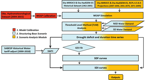
In the second module, the water deficit is defined from the WEAP historical simulation dataset and the assumptions of stationary (SD) and non-stationary (NSD) water demand scenarios to follow the severity–duration–frequency curves (SDF) approach (Sung and Chung 2014). The threshold level method (TLM) was applied to depict the main characteristics of drought events (mean duration and mean severity) over the historical period for the two proposed demand scenarios (Heudorfer and Stahl 2017; Rivera, Araneo, and Penalba 2017). Drought impact analysis is usually structured based on indices to measure the event magnitude and its consequences (Cambareri 2017). In this case, we develop the supply warranty time index (SWTI), on which an empirical relationship is established between the historical water deficit and extraordinary increases in water tariff prices. The SWTI is the ratio between the number of days in which all user sectors’ demand is met and the duration of the (intra-annual) drought event. As we show later on, we identified no water shortage up to the first 90 days of any drought event due to the system capacity; thus, SWTI is only below unity after 90 days of drought.

In the third module, the water utility profit losses are estimated under water deficit projections, driven by climate projections for the period of 2007–2040, 2041–2070, 2071–2099, and the water demand assumptions (SD–NSD).

3.1. Model calibration

The WEAP is an integrated water resource planning tool used to develop and assess scenarios that explore physical changes (natural or anthropogenic) and has been widely used in various basins worldwide (Yates et al. 2005). Climate-driven models such as WEAP provide dynamic tools by incorporating hydro-climatological variables to analyze, in this case, a one-dimensional, quasi-physical water balance model, which depicts the semi-distributed hydrologic response through the surface runoff, infiltration, evapotranspiration (Penman-Monteith equation), interflow, percolation, and base flow processes (Forni et al. 2016).

The hydrological model for the CWSS drainage area comprises 16 sub-basins with a spatial resolution ranging from 67 to 272 km² (Figure 1), which defines the natural discharge produced by the CWSS. The observed hydrologic data (discharge and rainfall) were obtained from HIDROWEB¹ (the National Water Agency database [ANA]), SABESP, and the São Paulo State Water and Electricity Department [DAEE]. A network of 52 rain gauge stations and 11 discharge gauge stations was configured, with inputs and outputs in a monthly time step (Figure 1(a,b)). Meteorological data from 14 gauging stations (temperature, relative humidity, wind speed, and cloudiness fraction) were obtained from the National Institute of Meteorology and Center for Weather Forecasting and Climate Research (CPTEC) databases (Figure 1(c)). For the basin characterization, we adopted the soil map from (De Oliveira, Marcelo Camrago, and Calderano Filho 1999) (scale 1:500,000) and the land use map of 2010 from (Molin et al. 2015) (scale 1:60,000).

The modeling process was carried out over 12 years, explained as follows: 24 months as a warm-up period (from 2004 to 2005), 60 months as a calibration period (from 2006 to 2010), and 56-months as a validation period (from 2011 to 2015). Although more extensive periods of calibration and validation are suggested to better represent hydrological dynamics (Gibbs et al. 2018), this first trial of warm-up with calibration and validation seems appropriate with the objectives of the study, restricted to the observed data and assessment periods.

The model was calibrated using a mixed calibration process. The first calibration approximation was made using the model-independent parameter estimation and uncertainty analysis software (PEST) (Doherty and Skahill 2006), followed by refinement using a manual adjustment technique. The following variables were calibrated: Kc (Crop Coefficient), SWC (soil water capacity), DWC (deep water capacity), RZC (root zone conductivity), DC (deep conductivity), and PFD (preferential flow direction (PFD). The objective functions to measure model performance, widely used in hydrologic applications, were the volumetric error percent bias (PBIAS) and the Nash-Sutcliffe efficiency (NSE) of the logarithmic of discharges (NSE_Log), which is more sensitive to low flows (Muleta 2012).

Although the model was delineated as 16 sub-basins, 11 of these units had discharge information, four of which coincided with the reservoir entry flow measures (see Figure 1, Jaguarí-Jacareí B5-B8, Cachoeira B9, and Atibainha B102 Subsystems). To manage water resources, SABESP considers the catchment’s natural inflows and the demanded downstream flow to estimate the available flow for the SPRM supply. The system operation is based on the integration of the four reservoirs through a balance called ‘Equivalent System’, this ES can be expressed as follows:

(1) $E{S}_{Cantareira}=\sum _i^{n}Q{N}_i-\sum _i^{n}W{D}_i$(1)

where ES_Cantareira is the available water for withdrawal from the system, QN is the natural discharge from each reservoir i (subsystem), and WD is the water demand in each reservoir (including downstream supply).

Once calibrated, the WEAP model was driven by the regional climate model (RCM) ETA-INPE reference period (1961–2005) to generate the baseline scenario. Details of ETA-INPE are addressed in Section 3.3.

3.2. Structuring base scenario module

The threshold level method (TLM) is traditionally used to estimate hydrological deficit events from the discharge time series (Wanders, Van Loon, and Van Lanen 2017). TLM was originally called ‘Crossing Theory Techniques” and it is also referred to as run-sum analysis (Şen 2015).

In this study, two monthly time-step thresholds were implemented, defined from the pre-established water demand in the system (Sung and Chung 2014). Initially, a stationary demand (SD) threshold of 31 m³/s is defined as equal to the historical average demand, and another non-stationary demand (NSD) threshold of 31 to 42 m³/s is defined as a hypothesis representative of the population growth in the SPRM (IBGE²) (Deusdará-Leal et al. 2020). Meanwhile, the discharge series are defined from the WEAP hydrological simulation driven by the Eta-INPE historical dataset scenarios (baseline period 1962–2005).

Based on the deficit time series (severity in m³) and duration (days) obtained from the TLM evaluation, the SDF curves were developed. The generalized extreme value (GEV) frequency distribution was used to estimate the return periods of the deficit events. The GEV distribution is useful because it includes all three types of extreme-value distributions (Tung, Yen, and Melching 2006). In various studies addressing SDF curve development, the GEV distribution is consistent with the datasets of extremes (Sophie Bachmair et al. 2017; Todisco, Mannocchi, and Vergni 2013; Sung and Chung 2014). To specify a considerable number of events to configure the SDF curves, the deficit duration was classified into four intervals from 0 days to 31 days, 0 days to 90 days, 0 days to 180 days, and 0 days to 365 days. Thus, the GEV parameters ξ, α, and µ were estimated using the maximum likelihood estimator (MLE) for the four duration intervals and return periods of 2, 10, and 100 years.

In Brazil, each state-owned sanitation company has its own water charging policy, where the vast majority use block tariffs as a pricing policy, including SABESP (De Andrade Filho, Ortiz, and de Oliveira 2015; Mesquita and Ruiz 2013). In Sao Paulo State, the tariff policy system is regulated by Decree 41.446/96, as well as by services provided by SABESP. For the water tariff setting, several factors are taken into account, such as service costs, debtors forecast, expenses amortization, environmental and climatic conditions, quantity consumed, user sectors, and economic condition of the user. These user sectors are divided into residential, industrial, and commercial sectors, and the value charged for the service is always progressive. In other words, there is a standard minimum consumption with a fixed value, and such factors vary the consumption ranges (SABESP 2018). From the total water withdrawn from the CWSS, urban use is predominant in SPRM, where approximately 49% of the total is for household needs, 31% is for industrial needs, and 20% is for irrigation (Consórcio PCJ 2013). In this study, we consider the water withdrawal for domestic and industrial use in the SPMR, due to the direct dependence of these sectors on the SABESP water supply network, as well as the supply priority that the domestic sector has according to Brazilian law during drought periods (Brasil 1997).

Urban drought management programs incur costs that must be assumed to overcome water crises with equity (Molinos-Senante and Donoso 2016). SABESP in the SPMR, for example, through price-based policies,³ controlled the consumption rates of users when hydrological deficit scenarios were presented in the CWSS. Therefore, during 2014/2015, reactive economic contingencies were implemented, such as increased water tariffs, extra fees, and price incentives. These had a detrimental effect on the company’s profit margin (SABESP, GESP 2016; SABESP 2017a, 2016a).

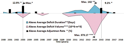
We established a drought revenue loss cost estimation method based on the market price method (Meyer et al. 2013). Although the financial impacts do not always exhibit a strong correlation with weather indices (Zeff and Characklis 2013), we developed an empirical relationship between water price (impacts) and drought (Mens, Gilroy, and Williams 2015; Grafton and Ward 2008; Hou et al. 2018; S Bachmair et al. 2016; Guzmán, Mohor, and Mendiondo 2020a). Figure 3 shows an increase in the adjustment rate as a response to periods of water deficit. Based on the TLM approach, we assessed the monthly discharge time series under SD (31 m³/s) from 2000 to 2018 (Figure 3), aiming to associate the drought characteristics with the adjustment rates of SABESP. The upper part of Figure 3 shows the deficit duration in blue, and the black bars represent the extra rate adjustment over the average tariff, in this case due to climatic conditions during the drought events between 2000–2018 period. The lower part in pink represents the deficit volume for each drought duration during the same period. The Pearson correlation coefficient analysis between the adjustment rate and drought features did not show a large difference; the estimated values were 0.453 for drought duration and 0.481 for drought deficit. Although the correlation coefficient values were relatively low, the use of these drought characteristics is useful given the lack of information regarding drought and its economic impacts on the study area. In this sense, we adopted the duration of drought characterization, as it can be a better indicator of perception and social expectation than the accumulated water deficit volume (Kuil et al. 2016).

Figure 3. Empirical relationship between CWSS above-average deficit duration (blue-area in days), CWSS above-average deficit volume (pink-area in 10⁶-m³) and adjustment above-average adjustments rate (black-bars in percentage). modified from (Guzmán, Mohor, and Mendiondo 2020a).

Therefore, we adopted an empirical pricing structure adjusted to scarcity, from the average prices of the bulk water tariff in 2016 in the SPMR, for the domestic and industrial sectors integrating the resilience that the reservoir system can offer (SABESP, GESP 2016b). On the one hand, during the most severe droughts, an increase in the water tariff for the following period is expected to be a management measure. On the other hand, when smaller deficits are overcome with the water stored in the system, the increase in tariffs is a consequence of the annual consumer price index (CPI) and other tariff updates according to the law (SABESP, GESP 2016b). Thus, the approach requires the following additional assumptions:

• Based on the current average prices for the domestic and industrial sectors, a base water price was established to analyze US$ 3.38 per m³, assuming normal supply conditions or 100% water availability.

• From the SDF curve construction intervals (cumulative drought duration) and three class intervals of the annual tariff adjustment (6%, 10%, and 17%, see Figure F-1 and Table F-1 in Supplementary Material F), the water prices were established.

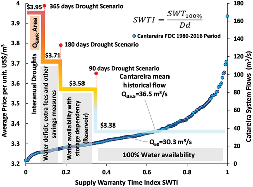
The analysis focuses on quantifying the impacts of a variety of drought events by integrating the operational capacity of the system (Mens, Gilroy, and Williams 2015). From the reconstructed and observed flow series of the CWSS between 1930 and 2016 (ANA/DAEE 2013), flow duration curves for different historical periods were estimated (see Supplementary Material, Section G). The curves show a flow frequency reduction of what is currently extracted from the system (31 m³/s), denoting a gradual reduction over time. The flow had a permanence of 56% (Q₅₆) for the regime between 1930–1960 but had a permanence of only 49% between 1960–2016. Additionally, the flow duration curve 1980–2016 was analyzed as the current state of the system. This curve showed that the observed average flows in the years 2014 (8.71 m³/s) and 2015 (19.71 m³/s) are equivalent to the duration curve flows Q₉₈ and Q₇₈, which are generally related to hydrological drought phenomena or low supply.

Our robustness analysis was defined around a pricing policy delimited for three staggered tariff-adjustments to face the drought duration scenarios represented by the SWTI (Figure 4). First, in a scenario of 100% water availability, the continuous flow balances the water inlet and outlet in the reservoir network to ensure supply (drought duration up to 90 days). Second, there is a scenario with water availability and supply warranty and dependence on the storage system. In this scenario, the reservoir network provides resilience during droughts of smaller magnitudes and durations, maintaining supply with a low tariff adjustment (drought durations between 90 and 180 days). Third, a scenario with water shortage, and consequently, forced interruption of supply. In this scenario, the water deficit prevails with a high tariff adjustment and other savings measures (drought durations between 180 and 365 days).

Figure 4. Pricing structure adjusted to scarcity: where SWT_100% is number of days that 100% of supplies can be guaranteed once the drought event has started and D_d the duration of the intra-annual drought event and FDC is the flow duration curve to CWSS. modified from Guzman, Mohor and Mendiondo (2020).

Finally, the link between the deficit and company profit losses due to business interruption during unavailability water periods is given by means of the SDF curves. The pricing structure and deficit share the same event duration. Thus, this approach offers a set of alternatives for impact analysis of different magnitudes and climate scenarios.

3.3. Scenario analysis module

Once the WEAP hydrological model has been calibrated and validated and the relationship between drought and tariff adjustment has been established, we calculate the drought impacts (WUBIC) through the management horizons (2007–2040, 2041–2070, and 2071–2099). This calculation was carried out for cumulative deficit periods greater than 180 days of drought using the TLM approach for all WEAP simulations. A drought value of 180 days was defined considering that, from this duration, the supply begins to show an important dependence on the CWSS.

To incorporate the uncertainties of climate change impacts, historical simulations and future projections of the RCM Eta-INPE model were used. Currently, the RCM Eta-INPE (Brazilian National Institute for Space Research) plays an important role in providing information for local impact studies in Brazil and other areas of South America (Chou et al. 2014a). The RCM model is nested within the GCMs MIROC5 and HADGEM-ES, forced by two greenhouse gas concentration scenarios (RCPs) 8.5 and 4.5 [W/m²] (used in the IPCC 5th Assessment Report), with a horizontal grid size resolution of 20 km × 20 km and up to 38 vertical levels through 30 years of time periods, distributed as follows: 1961–2005 (as the baseline period), 2007–2040, 2041–2070 and 2071–2099 (Chou et al. 2014a; Prudhomme et al. 2014). It should be clarified that, for the future periods, the growth in water consumption under the NSD assumption is implemented progressively; that is, for 2005–2040 it is attributed an average water withdrawal of 31 m³/s, 38 m³/s for 2041–2070, and 43 m³/s for 2071–2099.

4. Results and discussion

4.1. Hydrological model fit

It is worth noting that the sub-basin areas in this case are smaller than each cell of the adopted climate model (400 km²), although RCMs are an alternative to downscale the coarse-resolution GCM, RCM outputs often deviate from the observed climatological data (Liersch et al. 2016; Kim, Kwon, and Han 2015; Smitha et al. 2018). Therefore, the historical simulation and, consequently, the future projections of Eta-INPE had to be spatially relocated and bias corrected from observed historical climate conditions (rain and temperature). For this, the ‘Additive Corrections and Scaling’ method was used, which is a simple approach that assumes the relative mean biases between observed data and model projections (Maraun and Widmann 2018; Smitha et al. 2018).

The hydrological model structure was performed in monthly time steps and was calibrated and validated following the procedure described in Section 3.1. Multiple statistical evaluation criteria were used to improve the calibration procedure (Kumarasamy and Belmont 2017; Gibbs et al. 2018). This is important because analyzing multiple statistics can provide an overall view of the model based on a comprehensive set of indexes on the parameters representing the statistics of the mean and extreme values of the hydrograph (Moriasi et al. 2007). The equivalent system hydrographs for the calibration and validation periods are shown in Figure 5. The colors in Figure 5 represent the classifications suggested by Moriasi et al. (2007) and are as follows: green for ‘very good’ (NSE > 0.75; PBIAS < ±10%; RSR < 0.50), yellow for ‘good or satisfactory’ (0.75 > NSE > 0.5; ±10% < PBIAS < ±25%; 0.50 < RSR < 0.60), and red for ‘unsatisfactory’ (NSE < 0.5; PBIAS > ±25%; RSR > 0.70). Moreover, the correlation coefficient (R²) and VE criterion values close to 1.0, indicate that the prediction dispersion is equal to that of the observation (Muleta 2012; Krause and Boyle 2005). It is important to note that during the validation period (2011–2015), most of the recent drought events were simulated with an acceptable performance, although there was a tendency to overestimate periods of low flow.

Figure 5. WEAP hydrographs cantareira Equivalent System (ES) performance criteria for calibration (2006 − 2010) – validation (2011–2015) periods. the calibration and validation performance criteria for each sub-basin in the system can be found in supplementary material B. – Table B-1.

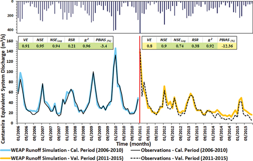
Later, in the impact assessment, only the equivalent system (ES) was analyzed. Among the simulated subsystems, the Jaguarí-Jacareí subsystem contributes to approximately 46% of the total water production and shows the best modeling performance statistics, compared to the other subsystems. The SE discharge projections 2007–2099 forced by the GCM and RCP scenarios can be seen in the Supplementary Material (Fig. C-1).

4.2. Droughts severity-duration-frequency and -impact curves

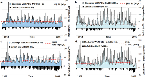
Figure 6 shows the baseline (historical) scenario results of the TLM approach for each GCM (Eta-MIROC5 and Eta-HadGEM-ES) simulations and under the thresholds SD and NSD. In general, the results driven by Eta-MIROC5 showed the greatest deficits under the two threshold scenarios. On the other hand, the Eta-HadGEM-ES simulation through the SD threshold proved to be an optimistic scenario in terms of low deficits and drought durations.

Figure 6. TLM approach from historical WEAP´s simulation driven by RCM Eta (base line scenarios) under Stationary (SD) and Non-Stationary Demand (NSD) threshold assumptions: a. 31 m3/s and Eta-MIROC5. b. 31 m3/s and Eta-HadGEM-ES. c. 31 to 42 m3/s and Eta-MIROC5. d. 31 to 42 m3/s and Eta-HadGEM-ES.

The left side of Figure 7 shows the SDF curves for the historical period scenarios of the GCM and water demand fit for the return periods (Rp) of 2, 10, and 100 years. It can be observed from the results that according to the fit data set (Supplementary Material D), the shape parameter (ξ) varies with the drought duration. For a drought interval of more than 180 days, the probability distribution function (PDF) Type I presents a better fit, whereas droughts with duration intervals of less than 90 days had a better fit to FDP Type III (see Tables E-1 to E-4 in Supplementary Material E). Moreover, the fit diagnostic plots ‘Empirical quantile vs Model quantile’ (QQ-plot) and ‘Return level vs Return period’ (RR-plot) show the relationship between the model, the data fit and prediction capacity (Supplementary Material D). Therefore, in terms of the quantiles, the QQ plot shows the data trend to follow the model line in most cases, while the predictive capacity of the model, represented by the RR-plot, shows a decrease as the return period increases.

Figure 7. Severity-Duration-Impact (SDI) curves. panel a. severity-duration-frequency-profit loss under the historical Eta-MIROC5 scenario. sector b. severity-duration-frequency-profit loss under the historical Eta-HadGEM-ES scenario. Note: SD and NSD are the stationary or non-stationary demands, respectively; ‘VD’ is the volume deficit, under return period of 2, 10 and 100 years; % of year is the drought event duration in relation to one year.

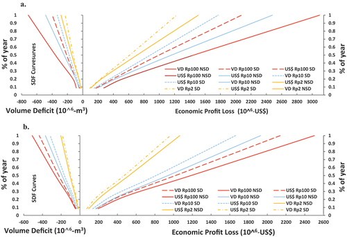
Based on the duration of the drought as a common element between the CWSS SDF curves and the pricing structure adjusted to scarcity, the functions of the (SDI) were built. The right side of Figure 7 shows the intra-annual drought duration as the progress percentage throughout the year, deficit, and consequent company profit losses. SDI functions are structured to analyze the impact under different magnitude events (represented by Rp), climate projections (RCPs – GCMs), and demand variability scenarios (SD – NSD). The curve set represents the uncertainty associated with the drivers considered. Each pair of lines in Figure 8 (continuous and dashed lines) shows the range of possible impacts generated by water scarcity across demand scenarios.

Figure 8. Impacts and relative differences between scenarios. Medians (Med.) and standard deviations (σ). panel ‘a’: impacts based on RCP scenarios. panel ‘b’: impacts based on RCM scenarios. panel ‘c’: impacts based on demand scenarios. through analysis periods, first panel 2007–2040, second panel 2041–2070 and third panel 2071–2099.

4.3. Water utility company impacts

The results here describe the net present value (NPV) of the potential economic impacts represented in SABESP revenue losses related to hydrological drought durations greater than 180 days. The set of impacts was organized by differentiating results from climate projections, demand scenarios, drought severity (accumulated deficit), and recurrence scenarios during the analyzed periods: 2007–2040, 2041–2070, and 2071–2099. The evaluation of the drought’s economic impact projections in SABESP showed, in general, revenue losses per analysis period between 0.003% and 0.021% of the SPMR GDP in 2017. This relatively low range of percentage revenue losses is, in fact, significant for the regional economy, since SPMR accounts for approximately 18% of the Brazilian GPD.

The results in Figure 9 show that under the water demand driver, the most conducive scenarios are configured to generate the greatest impacts on average. This was expected, given the proposed non-stationary threshold demand. In descending order, the lowest economic impacts on average were observed under RCP and GCM drivers, respectively. Likewise, in Panel ‘a’, the impacts analyzed under RCP scenarios 4.5 and 8.5 showed a low difference percentage in variability and median. This can be explained by the study by Chou et al. (2014a), where the Eta-INPE results establish that, in the future, there is no clear trend in the average precipitation. During the summer, the time series show a trend for a reduction in precipitation in both emission scenarios, RCP 8.5 and 4.5. For Panel ‘b’ (RCM), the outputs nested in Eta-MIROC5 presented higher revenue losses in the company than those based on Eta-HadGEM-ES. This difference can be attributed to the annual cycle of precipitation, which shows that the Eta-INPE simulations driven by MIROC5 generally produce less precipitation during the dry season; therefore, the water deficit during this period will be more critical (Chou, Lyra, Mourão, Dereczynski, Pilotto, Gomes, Bustamante, Tavares, Silva, Rodrigues, Campos, Chagas, Sueiro, Siqueira, Nobre, et al. 2014b). Finally, Panel ‘c’, where the NSD trend imposed the larger differences in the magnitude and variability percentage impacts (human influences), suggesting that the demand-related (population growth) uncertainty might be comparable to or larger than that associated with climate sensitivity.

Figure 9. Economic impacts comparison between Eta-INPE_RCP_GCM based scenarios throughout the projection time periods: first panel 2007–2040, second panel 2041–2070 and third panel 2071–2099.

Under a different grouping configuration for the analysis of the results (see Figure 9), the impact assessment was conditioned by the scenario joint study of climate forcing (Eta-GCM) and radiation (RCP). Based on this scheme, it was found that the largest economic impact was represented by the Eta-MIROC5_4.5 climate-forcing scenario, while smaller impacts (on average) were observed in the Eta-HadGEM-ES_4.5 scenario. In addition, the Eta-MIROC5 scenario showed the maximum values of the median 50^th percentile (Max.-Med.) and standard deviation (Max.SD) between the set of period panels, which concludes that climate forcing based on the MIROC5 model is the main driver of the impacts and variability between analyzed climate drivers (GCM).

In all cases, the average impact projected for the period 2041–2070 was the lowest across periods. According to a study by Lyra et al. (2017), in which the most recent Eta-INPE model simulations were performed at more detailed scales, the annual total precipitation (PRCPTOT) and maximum number of consecutive days with precipitation (CDD-CWD) indices for the São Paulo region showed better results in terms of favoring water availability during this period. On the contrary, the period 2007–2040 presented the greatest impacts (evidence of the recent water crisis) and the lowest dispersion (less uncertainty). The 2071–2099 projection showed impacts similar to the 2007–2040 period, given that both Eta-INPE simulations intensify the reduction of precipitation toward the end of the century in Southeast Brazil, with an annual rainfall reduction above 40% and a reduction in precipitation extremes (Lyra et al. 2017; Chou et al. 2014a).

In this work, we have addressed the WUBIC to hydrological droughts and its association with multiple drivers, such as climate change and water demand. Nonetheless, previous works have shown the economic risk of hydrological drought for other user sectors (Guzmán, Mohor, and Mendiondo 2020), such as industrial, domestic, agricultural, and environmental (Mohor and Mendiondo 2017), and its effect on the design of insurance instruments. The results therein show that the drivers of change coupled with the national normative, which establishes the sectorial priority of supply, can lead to high losses in the SPMR, especially in the industrial sector (Guzmán, Mohor, and Mendiondo 2020). Fair insurance premiums to cope with drought financial impacts can surpass 0.4% of local GDP (Guzman 2018), showing that both the water utility company and its users are vulnerable to water insecurity and consequent impacts.

4.4. Considerations on uncertainties

The methodology adopted here includes a model chain, which is typical for hydrological regime projection exercises through hydrologic simulation under climate change projections (Jones 2000; Wilby and Harris 2006; Fowler, Blenkinsop, and Tebladi 2007; Hoque et al. 2019). This model chain incorporates several sources of uncertainty, such as those listed by Honti, Scheidegger, and Stamm (2014) and Jobst et al. (2018), 1) the climate model; 2) the downscaling method or an RCM application, the latter as in our work; 3) the hydrological model; and (4) the inherent modeling uncertainty of coupling different climate-hydrology spatiotemporal scales.

In this case, the systematic analysis of change drivers (uncertainty sources) offers a set of results around potential scenarios to frame uncertainty (Refsgaard et al. 2007; Rodrigues et al. 2015), while the driver sensitivity analysis is proposed as a part of the results of this study. Montanari (2007), however, advocates that some methods commonly used for uncertainty assessment do not address uncertainty, but only model sensitivity. Moreover, although some studies indicate that climate projections surpass hydrological uncertainties (Bates et al. 2008; Nóbrega et al. 2011), Honti, Scheidegger, and Stamm (2014) reinforce that different methods of uncertainty assessment may lead to different conclusions. The uncertainty associated with the drivers of change is represented in cost terms (WUBIC) by period (2018–2040, 2041–2070, and 2071–2099) around 9,206 US $ x10⁶, 8,616 US $ x10⁶ and 11,975 US $ x10⁶, respectively.

Our methodology also included a drought indicator development through the TLM approach, demand scenarios, and a drought cost estimation based on the market price method (Mens, Gilroy, and Williams 2015; Hou et al. 2018). The results showed that drought deficits are influenced not only by the modeled inflows at a lumped scale, throughout the period–2007-2099, but also in our case study by reservoir operation. In fact, the spatially combined operation of existing reservoirs may be different from our considerations, adopting an ‘equivalent system’ (ES) without a future layout change. On the one hand, the system demand scenarios are based on the best current knowledge (historical period: 2004–2016, (SABESP 2017b)) and the adoption of two scenarios aimed at providing a broader, realistic view of the different possible outcomes due to expected population growth (Hou et al. 2018). On the other hand, economic loss estimation, based on the aforementioned drought event measures, does not incorporate eventual market changes, currency changes, or even subsidies. Conversely, our loss estimation assumes that those economic measures, that is, water tariff adjustments, were and would continue to be adopted by the water utility, as a trigger determinant once the drought hazard occurred. Because this triggering factor would temporarily occur either promptly or slowly, when structural measures were not sufficient to secure water supply under eventual hydro-meteorological conditions and water demand, uncertainties in cost analysis could increase.

5. Conclusion and recommendations

In this paper, we presented a multi-driver ensemble to assess the economic impacts of water utility triggered by climate change and demand variability. Methodologically, we first characterized hydrological droughts through the SDF curves from the baseline period. Second, an empirical drought economic impact curve was set up, representing the water utility company profit loss due to unmet demand during hydrological drought periods coupled with tariff adjustments through the SWTI developed here. Additionally, our results have further implications for drought risk reduction and management.

The implemented methodology revealed SPMR water insecurity against hydrological droughts. It is possible that the maximum supply capacity of the system is reaching its limit owing to the growing demand and the new challenges represented by climate change. On the one hand, the main driver of economic impacts turned out to be water demand dynamics. In contrast, the radiation scenarios showed no major differences. The scenarios analyzed here do not comprise the full variability of climate projections, and the two GCMs were shown to be a large source of uncertainty. Thus, a larger number of GCMs are highly recommended. However, the water demand scenario, which is aligned with population growth estimates and is comparatively less uncertain, directly leads to an increase in drought impacts.

The approach presented here could be expanded to analyze the impacts of key drivers such as land use and link interdisciplinary studies with broader relationships in relation to water, energy, and food security. The inclusion of more gauge stations could not only improve the calibration performance but also cover a larger sample space of events, increasing the confidence of projections. Similarly, the reliability of SDF curve estimates depends on the quality and extent of the records used, or in this case, the capacity of RCMs to reproduce the distribution of extreme events. The methodology assimilates consecutive years of water deficit independently. Nonetheless, introducing a direct measure of the economic impacts resulting from a multi-year drought event could improve the estimates. Drivers such as demand variability indicate an important uncertainty to financial resilience; for example, recent reductions in water demand in commercial, industrial, and institutional sectors, due to the pandemic, generated a reduction in the income of water companies. The scenarios analyzed here can assist the decision-making of water utility companies to cope with the economic impacts of drought risks in the long and medium term. The expected profit loss over the long term serves as the initial estimate for financial contingency arrangements such as insurance schemes or community contingency funds. In general, the approach developed here can be proposed as a planning tool to mitigate drought-related revenue losses, as well as being useful for the development of water resource securitization strategies in sectors highly dependent on water.

Acknowledgements

The first author would like to express its gratitude to the Administrative Department of Science, Technology, and Innovation (COLCIENCIAS) Doctoral Program Abroad – Colombia. We would also like to thank the Brazilian research agencies: CAPES-PROEX-PPG-SHS, Pró-Alertas #88887.091743/2014-01, CNPq #307637/2012-3, CNPq #312056/2016-8 (PQ) and CNPq #465501/2014-1 (“Segurança Hídrica”, Water Security of the INCT-Climate Change II.), FAPESP #2014/15080-2, FAPESP #2014/50848-9 and The Sao Paulo State Water Utility Company, SABESP, kindly provided relevant information for this study. The third author thank to Coordination of Superior Level Staff Improvement (CAPES) and to the Programme of Postgraduate in Hydraulics and Sanitation (PPG-SHS) for the postdoctoral fellowship.

Supplementary material

Supplemental data for this article can be accessed https://doi.org/10.1080/1573062X.2022.2058564

Correction Statement

This article has been corrected with minor changes. These changes do not impact the academic content of the article.

Notes

1. https://www.snirh.gov.br/hidroweb/apresentacao.

2. Brazilian Institute of Geography and Statistics: http://www.ibge.gov.br/home/.

3. Database ‘percentage rate increase’ 2001–2018 SABESP: http://www.sabesp.com.br/CalandraWeb/CalandraRedirect.

References

- Agencia das Bacias PCJ, Comitês PCJ. 2016. Capivari e Jundiaí Ano Base – 2015. Sao Paulo: Agencia das Bacias PCJ.
- Ali, Ghaffar, Muhammad K Bashir, Sawaid Abbas, and Mehwish Murtaza. 2021. “Drinking-Water Efficiency, Cost of Illness, and Peri-Urban Society: An Economic Household Analysis.” PLoS One 16 (e0257509): 1–13. https://journals.plos.org/plosone/article?id=10.1371/journal.pone.0257509
- ANA/DAEE. 2013. Dados de Referência Acerca Da Outorga Do Sistema Cantareira. Sao Paulo: Departamento de Águas e Energia Elétrica - Agência Nacional de Águas e Saneamento Básico. http://arquivos.ana.gov.br/institucional/sof/Renovacao_Outorga/DadosdeReferenciaAcercadaOutorgadoSistemaCantareira.pdf
- Asadieh, Behzad, and Nir Y Krakauer. 2017. “Global Change in Flood and Drought Intensities under Climate Change in the 21st Century.” Hydrology and Earth System Sciences 21 (June): 5863–5874. doi:10.5194/hess-21-5863-2017.
- Ault, T. R. 2020. “Erratum: On the Essentials of Drought in a Changing Climate (Science D0I: 10.1126/Science.Aaz5492).” Science 368 (6489): 256–260. doi:10.1126/SCIENCE.ABC4034.
- Bachmair, S, C Svensson, J Hannaford, L J Barker, and K Stahl. 2016. “A Quantitative Analysis to Objectively Appraise Drought Indicators and Model Drought Impacts.” Hydrology and Earth System Sciences 20 (7): 2589–2609. doi:10.5194/hess-20-2589-2016.
- Bachmair, Sophie, Cecilia Svensson, Ilaria Prosdocimi, Jamie Hannaford, and Kerstin Stahl. 2017. “Developing Drought Impact Functions for Drought Risk Management.” Natural Hazards and Earth System Sciences 17 (11): 1947–1960. doi:10.5194/nhess-17-1947-2017.
- Balbus, John. 2017. “Understanding Drought’s Impacts on Human Health.” The Lancet Planetary Health 1 (1): e12. The Author(s). Published by Elsevier Ltd. This is an Open Access article under the CC BY license 10.1016/S2542-5196(17)30008-6.
- Bates, B.C., Z.W. Kundzewicz, S. Wu, and J.P. Palutikof.2018. “Climate Change and Water.“ Technical Paper of the Intergovernmental Panel on Climate Change, IPCC Secretariat, Geneva, 210 pp. https://archive.ipcc.ch/publications_and_data/publications_and_data_technical_papers.shtml
- Berman, Jesse D, Keita Ebisu, Roger D Peng, Francesca Dominici, and Michelle L Bell. 2013. “Articles Drought and the Risk of Hospital Admissions and Mortality in Older Adults in Western USA from 2000 to 2013: A Retrospective Study.” Lancet Planet Health 1 (1): e17–e25. The Author(s). Published by Elsevier Ltd. This is an Open Access article under the CC BY-NC-ND license 10.1016/S2542-5196(17)30002-5.
- Brasil, 1997. LEI No 9.433, DE 8 DE JANEIRO DE 1997 - PFEDERAL. LEI No 9.433, DE 8 DE JANEIRO DE 1997 - Política Nacional de Recursos Hidricos. n. Pdr 2020, p. 3901–3902, Política Nacional de Recursos Hidricos.
- Bressers, Hans, Nanny Bressers, and Corinne Larrue. 2016. “Introduction: Why Governance for Drought Resilience?” In Governance for Drought Resilience Land and Water Drought Management in Europe, Vol. 266. AG Switzerland: springer Open, 266. doi:10.1007/978-3-319-29671-5.
- Bucheli, Janic, Tobias Dalhaus, and Robert Finger. 2020. “The Optimal Drought Index for Designing Weather Index Insurance.” European Review of Agricultural Economics 1–25. doi:10.1093/erae/jbaa014.
- Buckeridge, M, and W Costa Ribeiro. 2018. LIVRO BRANCO DA ÁGUA A Crise Hídrica Na Região Metropolitana de São Paulo Em 2013-2015: Origens, Impactos e Solucoes. 1st ed. Sao Paulo: Instituto de Estudos Avançados da Universidade de São Paulo Academia de Ciências do Estado de São Paulo. http://www.iea.usp.br/publicacoes/ebooks/livro-branco-da-agua
- Cambareri, Grace 2017. “Robust Drought Planning in Megacities: A Case Study in São Paulo, Brazil.” University of Massachusetts Amherst.
- Cavalcanti, Iracema F A, and Vernon E Kousky. 2001. “Drought in Brazil during Summer and Fall 2001 and Associated Atmospheric Circulation Features.” Revista Climanálise 1: 1–10.
- Chou, Sin Chan, André Lyra, Caroline Mourão, Claudine Dereczynski, Isabel Pilotto, Jorge Gomes, Josiane Bustamante, et al. 2014a. “Assessment of Climate Change over South America under RCP 4.5 And 8.5 Downscaling Scenarios.” American Journal of Climate Change 3 (5): 512–527. doi:10.4236/ajcc.2014.35043.
- Chou, Sin Chan, André Lyra, Caroline Mourão, Claudine Dereczynski, Isabel Pilotto, Jorge Gomes, Josiane Bustamante, et al. 2014b. “Evaluation of the Eta Simulations Nested in Three Global Climate Models.” American Journal of Climate Change 3 (5): 438–454. doi:10.4236/ajcc.2014.35039.
- Consórcio PCJ. 2013. Sistema Cantareira : Um Mar de Desafios. Compilado de Textos, Informações e Subsídios Voltados a Renovação Da Outorga Do Sistema Cantareira. Sao Paulo. Versão 1.1 - Compilado de Textos, Informações e Subsídios voltados a Renovação da Outorga do Sistema Cantareira. http://agua.org.br/apresentacoes/71557_ApostilaCantareira-ConsorcioPCJ.pdf
- Coutinho, Renato M, Roberto A Kraenkel, and Paulo I Prado. 2015. “Catastrophic Regime Shift in Water Reservoirs and São Paulo Water Supply Crisis.” PLoS One 1–14. doi:10.1371/journal.pone.0138278.
- De Andrade, Claudia. 2016. Managing Water (In) Security in Brazil- Lessons from a Megacity. Vol. 44. London: Springer, Cham. doi:10.1007/978-3-319-56946-8_25.
- De Andrade Filho, Moises, Ortiz Javier, and Marcelo de Oliveira. 2015. “Water Pricing in Brazil: Successes, Failures, and New Approaches.” In Water Pricing Experiences and Innovations, edited by Ariel Dinar, Victor Pochat, Josè Albiac-Murilo, Stefano Farolfi, Rathinasamy Saleth, and Iss Global, 485. Vol. 9. Springer Cham Heidelberg New York Dordrecht London: Springer International Publishing Switzerland. doi:10.1007/978-3-319-16465-6.
- De Oliveira, João Bertoldo, Marco Rossi Marcelo Camrago, and Braz Calderano Filho. 1999. Mapa Pedológico Do Estado de São Paulo. 1 ed. Campinas: Embrapa, IAC.
- Deusdará-Leal, Karinne Reis, Luz Adriana Cuartas, Rong Zhang, Guilherme S. Mohor, Luíz Valério de Castro Carvalho, Carlos Afonso Nobre, Eduardo Mario Mendiondo, Elisângela Broedel, Marcelo Enrique Seluchi, and Regina Célia Dos Santos Alvalá. 2020. “Implications of the New Operational Rules for Cantareira Water System: Re-Reading the 2014-2016 Water Crisis.” Journal of Water Resource and Protection 12 (4): 261–274. doi:10.4236/jwarp.2020.124016.
- Doherty, John, and Brian E Skahill. 2006. “An Advanced Regularization Methodology for Use in Watershed Model Calibration.” Journal of Hydrology 327 (327): 564–577. doi:10.1016/j.jhydrol.2005.11.058.
- Falkenmark, M., and M. Lannerstad. 2004. “Consumptive Water Use to Feed Humanity – Curing a Blind Spot.” Hydrology and Earth System Sciences Discussions 1 (1): 7–40. doi:10.5194/hessd-1-7-2004.
- Forni, Laura G, Josué Medellín-azuara, Michael Tansey, Charles Young, David Purkey, and Richard Howitt. 2016. “Integrating Complex Economic and Hydrologic Planning Models_ an Application for Drought under Climate Change Analysis.” Water Resources and Economics 16 (October): 15–27. Elsevier 10.1016/j.wre.2016.10.002.
- Fowler, H.J., S. Blenkinsop, and C. Tebladi. 2007. “Review Linking Climate Change Modelling to Impacts Studies: Recent Advances in Downscaling Techniques for Hydrological Modelling.” International Journal of Climatology 4: 1549–1555. doi: 10.1002/joc. (December 2007).
- Freire-González, Jaume, Christopher Decker, and Jim W. Hall. 2017. “The Economic Impacts of Droughts: A Framework for Analysis.” Ecological Economics 132 (February): 196–204. Elsevier B.V 10.1016/j.ecolecon.2016.11.005.
- Gibbs, Matthew S., David McInerney, Greer Humphrey, Mark A. Thyer, Holger R. Maier, Graeme C. Dandy, and Dmitri Kavetski. 2018. “State Updating and Calibration Period Selection to Improve Dynamic Monthly Streamflow Forecasts for an Environmental Flow Management Application.” Hydrology and Earth System Sciences 22 (1): 871–887. doi:10.5194/hess-22-871-2018.
- Grafton, R. Quentin, and B. Ward Michael. 2008. “Prices versus Rationing: Marshallian Surplus and Mandatory Water Restrictions.” Economic Record 84 (SUPPL.1): 57–65. doi:10.1111/j.1475-4932.2008.00483.x.
- Guzman, Diego A. 2018. “Hydrological Risk Transfer Planning under the Drought ‘Severity- Duration-Frequency’ Approach as a Climate Change Impact Mitigation Strategy.” Sao Paulu Univeristy.
- Guzmán, Diego, A. Guilherme, S. Mohor, and M. Mendiondo Eduardo. 2020. “Multi-Year Index-Based Insurance for Adapting Water Utility Companies to Hydrological Drought: Case Study of a Water Supply System of the Sao Paulo Metropolitan Region, Brazil.” Water 12 (11): 2954. Multidisciplinary Digital Publishing Institute. doi:10.3390/w12112954.
- Heudorfer, B, and K Stahl. 2017. “Comparison of Different Threshold Level Methods for Drought Propagation Analysis in Germany.” Hydrology Research 48 (5): 1311–1326. doi:10.2166/nh.2016.258.
- Honti, M., A. Scheidegger, and C. Stamm. 2014. “The Importance of Hydrological Uncertainty Assessment Methods in Climate Change Impact Studies.” Hydrology and Earth System Sciences 18 (8): 3301–3317. doi:10.5194/hess-18-3301-2014.
- Hoque, Muhammad Ziaul, Shenghui Cui, Xu Lilai, Imranul Islam, Ghaffar Ali, and Jianxiong Tang. 2019. “Resilience of Coastal Communities to Climate Change in Bangladesh: Research Gaps and Future Directions.” Watershed Ecology and the Environment 1: 42–56. Elsevier B.V. 10.1016/j.wsee.2019.10.001.
- Hou, Wei, Zai Qing Chen, Dong Dong Zuo, and Guo Lin Feng. 2018. “Drought Loss Assessment Model for Southwest China Based on a Hyperbolic Tangent Function.”International Journal of Disaster Risk Reduction (January): 1. Elsevier Ltd 10.1016/j.ijdrr.2018.01.017.
- Ivana, Logar, and Jeroen C J M van den Bergh. 2012. “Methods to Assess Costs of Drought Damages and Policies for Drought Mitigation and Adaptation: Review and Recommendations.” Water Resources Management 27 (6): 1707–1720. doi:10.1007/s11269-012-0119-9.
- Jobst, Andreas M., Daniel G. Kingston, Nicolas J. Cullen, and Josef Schmid. 2018. “Intercomparison of Different Uncertainty Sources in Hydrological Climate Change Projections for an Alpine Catchment (Upper Clutha River, New Zealand).” Hydrology and Earth System Sciences 22 (6): 3125–3142. doi:10.5194/hess-22-3125-2018.
- Jones, Roger N. 2000. “Managing Uncertainty in Climate Change Projections – Issues for Impact Assessment.” Climatic Change 45 (3): 403–419. doi:10.1023/A:1005551626280.
- Kim, Kue Bum, Hyun Han Kwon, and Dawei Han.2015. “Bias correction methods for regional climate model simulations considering the distributional parametric uncertainty underlying the observations.“ Journal of Hydrology 530 (November): 568–579. doi:10.1016/j.jhydrol.2015.10.015.
- Krause, P, and D P Boyle. 2005. “Comparison of Different Efficiency Criteria for Hydrological Model Assessment.” Advances In Geosciences 5 (89): 89–97. doi:10.5194/adgeo-5-89-2005.
- Kuil, Linda, Gemma Carr, Alberto Viglione, Alexia Prskawetz, and Günter Blöschl. 2016. “Conceptualizing Socio-Hydrological Drought Processes: The Case of the Maya Collapse.” Water Resources Research 52 (8): 6222–6242. doi:10.1002/2015WR018298.
- Kumarasamy, Karthik, and Patrick Belmont. 2017. “Multiple Domain Evaluation of Watershed Hydrology Models.” Hydrology and Earth System Sciences Discussions, no. March: 1–32. doi:10.5194/hess-2017-121.
- Laaha, Gregor, Tobias Gauster, Lena M. Tallaksen, Jean-Philippe Vidal, Kerstin Stahl, Christel Prudhomme, Benedikt Heudorfer, et al. 2016. “The European 2015 Drought from a Hydrological Perspective.” Hydrology and Earth System Sciences Discussions 1–30. doi:10.5194/hess-2016-366.
- Liersch, Stefan, Julia Tecklenburg, Henning Rust, Andreas Dobler, Madlen Fischer, Tim Kruschke, Hagen Koch, and Fred Hattermann. 2016. “Are We Using the Right Fuel to Drive Hydrological Models? A Climate Impact Study in the Upper Blue Nile.” Hydrology and Earth System Sciences Discussions 1–34. doi:10.5194/hess-2016-422.
- Liu, Tingting, Richard Krop, Tonya Haigh, Kelly Helm Smith, and Mark Svoboda. 2021. “Valuation of Drought Information: Understanding the Value of the Us Drought Monitor in Land Management.” Water (Switzerland) 13 (2): 1–11. doi:10.3390/w13020112.
- Lloyd-hughes, Benjamin. 2013. “The Impracticality of a Universal Drought Definition.” Theoretical and Applied Climatology 117 (3–4): 6007–6611. doi:10.1007/s00704-013-1025-7.
- Lyra, Andre, Priscila Tavares, Sin Chan Chou, Gustavo Sueiro, Claudine Dereczynski, Marcely Sondermann, Adan Silva, and José Marengo. 2017. “Climate Change Projections over Three Metropolitan Regions in Southeast Brazil Using the Non-Hydrostatic Eta Regional Climate Model at 5-Km Resolution.” Theor Appl Climatol. Theoretical and Applied Climatology. doi:10.1007/s00704-017-2067-z.
- Maraun, D, and M Widmann. 2018. “Model Outputs Statistics.” In Statistical Downscaling and Bias Correction for Climate Research, First Edit, 170–200. London: Cambridge University Press. doi:10.1017/9781107588783.013.
- Marengo, Jose, Carlos A. Nobre, Marcelo Seluchi, Adriana Cuartas, Lincoln M Alves, E Mario Mendiondo, Guillermo Obregón, and Gilvan Sampaio. 2015. “A Seca e a Crise Hídrica de 2014-2015 Em São Paulo.” Revista USP 116 (106): 31–44. julho/agosto/setembro 2015 10.11606/.2316-9036.v0i106p31-44.
- Mehran, Ali, Omid Mazdiyasni, and Amir Aghakouchak. 2015. “A Hybrid Framework for Assessing Socioeconomic Drought: Linking Climate Variability, Local Resilience, and Demand.” Journal of Geophysical Reasearch: Atmospheres 7520–7533. doi:10.1002/2015JD023147.
- Mens, M. J. P., K. Gilroy, and D. Williams. 2015. “Developing System Robustness Analysis for Drought Risk Management: An Application on a Water Supply Reservoir.” Natural Hazards and Earth System Science 15 (8): 1933–1940. doi:10.5194/nhess-15-1933-2015.
- Mesquita, Arlan Mendes, and Ricardo Machado Ruiz. 2013. “A Financial Economic Model for Urban Water Pricing in Brazil.” Urban Water Journal 9006 (September): 85–96. doi:10.1080/1573062X.2012.699073.
- Meyer, V., N. Becker, V. Markantonis, R. Schwarze, J. C J M Van Den Bergh, L. M. Bouwer, P. Bubeck, et al. 2013. “Review Article: Assessing the Costs of Natural Hazards-State of the Art and Knowledge Gaps.” Natural Hazards and Earth System Science 13 (5): 1351–1373. doi:10.5194/nhess-13-1351-2013.
- Mishra, Ashok K., and Vijay P. Singh. 2010. “A Review of Drought Concepts.” Journal of Hydrology 391 (1–2): 1–2. Elsevier B.V.: 202–216 10.1016/j.jhydrol.2010.07.012.
- Mohor, Guilherme Samprogna, and Eduardo Mario Mendiondo. 2017. “Economic Indicators of Hydrologic Drought Insurance under Water Demand and Climate Change Scenarios in a Brazilian Context.” Ecological Economics 140: 66–78. Elsevier B.V. 10.1016/j.ecolecon.2017.04.014.
- Molin, Paulo Guilherme, Frederico Tomas De Souza, Paulo Guilherme Molin, Frederico Tomas De Souza, Jéssica Villela Sampaio, and Aline Aparecida. 2015. Mapeamento de Uso e Cobertura Do Solo Da Bacia Do Rio Piracicaba, SP: Anos 1990, 2000 e 2010. Sao Paulo: IPEF-Instituto de Pesquisas e Estudos Florestais. http://www.ipef.br/publicacoes/ctecnica/
- Molinos-Senante, María Mar??a, and Guillermo Donoso. 2016. “Water Scarcity and Affordability in Urban Water Pricing: A Case Study of Chile.” Utilities Policy 43: 107–116. Elsevier Ltd. 10.1016/j.jup.2016.04.014.
- Montanari, A. 2007. “What Do We Mean by ‘Uncertainty’? The Need for a Consistent Wording about Uncertainty Assessment in Hydrology.” Hydrological Processes 21 (6): 841–845. doi:10.1002/hyp. January 2007.
- Montanari, A., G. Young, H.H.G. Savenije, D. Hughes, T. Wagener, L.L. Ren, D. Koutsoyiannis, et al. 2013. “‘Panta Rhei—Everything Flows’: Change in Hydrology and Society—The IAHS Scientific Decade 2013–2022.” Hydrological Sciences Journal 58 (6): 1256–1275. doi:10.1080/02626667.2013.809088.
- Moriasi, D.N., J.G. Arnold, M.W. Van Liew, R.L. Binger, R.D. Harmel, and T.L. Veith. 2007. “Model Evaluation Guidelines for Systematic Quantification of Accuracy in Watershed Simulations.” Transactions of the ASABE 50 (3): 885–900. doi:10.13031/2013.23153.
- Muleta, M K. 2012. “Model Performance Sensitivity to Objective Function during Automated Calibrations.” Journal of Hydrologic Engineering 17 (6): 756–767. doi:10.1061/(ASCE)HE.1943-5584.0000497.
- Nam, Won-Ho, Michael J. Hayes, Mark D. Svoboda, Tsegaye Tadesse, and Donald A. Wilhite. 2015. “Drought Hazard Assessment in the Context of Climate Change for South Korea.” Agricultural Water Management 160: 106–117. Elsevier B.V. 10.1016/j.agwat.2015.06.029.
- Nobre, Carlos A., and Jose A. Marengo. 2016. Water Crises and Megacities in Brazil: Meteorological Context of the São Paulo Drought of 2014-2015. Brazil: Global Water Forum. Posted on October 17, 2016 in Climate Change, Environment, Urban Water, Water Security. Global Water Forum http://www.globalwaterforum.org/2016/10/17/water-crises-and-megacities-in-brazil-meteorological-context-of-the-sao-paulo-drought-of-2014-2015/
- Nobre, Carlos A., Jose A. Marengo, Marcelo E. Seluchi, Adriana Cuartas, and Lincoln M Alves. 2016. “Some Characteristics and Impacts of the Drought and Water Crisis in Southeastern Brazil during 2014 and 2015.” Journal of Water Resource and Protection 8 (February): 252–262. doi:10.4236/jwarp.2016.82022.
- Nóbrega, M. T., W. Collischonn, C. E. M. Tucci, and A. R. Paz. 2011. “Uncertainty in Climate Change Impacts on Water Resources in the Rio Grande Basin, Brazil.” Hydrology and Earth System Sciences 15 (2): 585–595. doi:10.5194/hess-15-585-2011.
- PCJ/Comitês. 2006. Fundamentos Da Cobrança Pelo Uso Dos Recursos Hídricos Nas Bacias PCJ. Sao Paulo: Comitês das Bacias Hidrográficas dos rios Piracicaba, Capivari e Jundiaí.
- Prudhomme, Christel, Ignazio Giuntoli, Emma L Robinson, Douglas B Clark, Nigel W Arnell, Rutger Dankers, Balázs M Fekete, et al. 2014. “Hydrological Droughts in the 21st Century, Hotspots and Uncertainties from a Global Multimodel Ensemble Experiment.” PNAS 111 (9): 3262–3267. doi:10.1073/pnas.1222473110.
- Refsgaard, Jens Christian, Jeroen P. van der Sluijs, Anker Lajer Højberg, and Peter A. Vanrolleghem. 2007. “Uncertainty in the Environmental Modelling Process - A Framework and Guidance.” Environmental Modelling and Software 22 (11): 1543–1556. doi:10.1016/j.envsoft.2007.02.004.
- Rivera, Juan A., Diego C. Araneo, and Olga C. Penalba. 2017. “Threshold Level Approach for Streamflow Drought Analysis in the Central Andes of Argentina: A Climatological Assessment.” Hydrological Sciences Journal 62 (12): 1949–1964. Taylor & Francis: 1949–1964 10.1080/02626667.2017.1367095.
- Rodrigues, Dulce B.B, Hoshin V Gupta, Eduardo M Mendiondo, and Paulo T S Oliveira. 2015. “Assessing Uncertainties in Surface Water Security: An Empirical Multimodel Approach.” Water Resources Research 51 (11): 9127–9140. doi:10.1002/2014WR016259.
- SABESP, GESP-Goberno do Estado de Sao Paulo. 2016. Relatório Da Administração 2016 - Companhia de Saneamento Básico Do Estado de São Paulo - SABESP. Sao Paulo. https://site.sabesp.com.br/site/uploads/file/sociedade_meioamb/relatorio_sustentabilidade_2016.pdf
- SABESP. 2016a. Comunicado - 02/16: Deliberação No 641/2016 Autorizando o Cancelamento Do Programa de Incentivo à Redução Do Consumo de Água. Sao Paulo: Goberno Estadual.
- SABESP, GESP. 2016b. “COMUNICADO - 03/16: Marco Tarifario RMSP 2016.” Comunidado 03/16: Tarifas Agua/Esgoto 2016. http://site.sabesp.com.br/site/uploads/file/clientes_servicos/comunicado_03_2016.pdf
- SABESP. 2017a. Relatório Da Administração 2017. Sao Paulo.
- SABESP. 2017b. “Sistema Cantareira.” Sistema Cantareira - Visualizar Sistema Equivalente. http://www2.ana.gov.br/Paginas/servicos/saladesituacao/v2/SistemaCantareira.aspx
- SABESP. 2017c. Relatório Da Administração 2017. Sao Paulo. http://www.dsaldo.com.br/EMPRESAS/Agua/Ciasaneamento/DFP2017.pdf
- SABESP. 2018. Tarifas. Accessed 05 December 2018. file:///C:/Users/LEGION/AppData/Local/Mendeley%20Ltd/Mendeley%20Desktop/Downloaded/SABESP%20-%202018%20-%20Regulamento%20do%20Sistema%20Tarif%C3%A1rio%20da%20Sabesp.html
- Sahin, Oz, Edoardo Bertone, Cara Beal, and Rodney A Stewart. 2018. “Evaluating a Novel Tiered Scarcity Adjusted Water Budget and Pricing Structure Using a Holistic Systems Modelling Approach.” Journal of Environmental Management 215: 79–90. Elsevier Ltd. 10.1016/j.jenvman.2018.03.037.
- Şen, Zekâi, ed. 2015. Applied Drought Modeling, Prediction, and Mitigation, 474. Amsterdam: Elsevier.
- Shi, Peijun, Jing’ai Wang, Xu Wei, Ye Tao, Saini Yang, Lianyou Liu, Weihua Fang, Kai Liu, Li Ning, and Ming Wang. 2015. Mapping Drought Risk (Maize) of the World. World Atlas of Natural Disaster Risk, 256. London: Springer. doi:10.1007/978-3-662-45430-5_17.
- Smakhtin, Vladimir U., and E. L F Schipper. 2008. “Droughts: The Impact of Semantics and Perceptions.” Water Policy 10 (2): 131–143. doi:10.2166/wp.2008.036.
- Smitha, P. S., B. Narasimhan, K. P. Sudheer, and H. Annamalai. 2018. “An Improved Bias Correction Method of Daily Rainfall Data Using a Sliding Window Technique for Climate Change Impact Assessment.” Journal of Hydrology 556: 100–118. Elsevier B.V. 10.1016/j.jhydrol.2017.11.010.
- Stahl, Kerstin, Irene Kohn, Veit Blauhut, Julia Urquijo, Lucia De Stefano, Vanda Acacio, Susana Dias, et al. 2016. “Impacts of European Drought Events: Insights from an International Database of Text-Based Reports.” Natural Hazards and Earth System Sciences 16 (3): 801–819. doi:10.5194/nhess-16-801-2016.
- Sung, J H, and E Chung. 2014. “Development of Streamflow Drought Severity – Duration – Frequency Curves Using the Threshold Level Method.” Hydrology and Earth System Sciences 18 (1997): 3341–3351. doi:10.5194/hess-18-3341-2014.
- Taffarello, Denise, Guilherme Samprogna Mohor, Maria Do Carmo Calijuri, and Eduardo Mario Mendiondo. 2016. “Field Investigations of the 2013–14 Drought through Quali-Quantitative Freshwater Monitoring at the Headwaters of the Cantareira System, Brazil.” Water International 8060 (August): 1–25. doi:10.1080/02508060.2016.1188352.
- Todisco, F, F Mannocchi, and L Vergni. 2013. “Severity – Duration – Frequency Curves in the Mitigation of Drought Impact: An Agricultural Case Study.” Natural Hazards 65 (3): 1863–1881. doi:10.1007/s11069-012-0446-4.
- Touma, Danielle, Moetasim Ashfaq, Munir A Nayak, Shih-chieh Kao, and Noah S Diffenbaugh. 2015. “A Multi-Model and Multi-Index Evaluation of Drought Characteristics in the 21st Century.” Journal of Hydrology 526: 196–207. Elsevier B.V. 10.1016/j.jhydrol.2014.12.011.
- Tung, Yeou-koung, Ben-Chie Yen, and Charles Melching. 2006. Hydrosystems Engineering Reliability Assessment and Risk Analysis, 512. 1st ed. New York: McGraw-Hill. doi:10.1036/0071451587.
- Ussami, Keyi Ando, and Joaquim José Guilhoto. 2018. “Economic and Water Dependence among Regions: The Case of Alto Tiete, Sao Paulo State, Brazil.” EconomiA 19 (3): 350–376. National Association of Postgraduate Centers in Economics, ANPEC 10.1016/j.econ.2018.06.001.
- Van Lanen, H A J, N Wanders, L M Tallaksen, A F Van Loon, and H A J Van Lanen. 2013. “Hydrological Drought across the World: Impact of Climate and Physical Catchment Structure.” Hydrology and Earth System Sciences 17 (17): 1715–1732. doi:10.5194/hess-17-1715-2013.
- Van Loon, Anne F. 2015. “Hydrological Drought Explained.” Wiley Interdisciplinary Reviews: Water 2 (4): 359–392. doi:10.1002/wat2.1085.
- Van Loon, Anne F., Tom Gleeson, Julian Clark, Albert I. J. M. Van Dijk, Kerstin Stahl, Jamie Hannaford, Giuliano Di Baldassarre, et al. 2016a. “Drought in the Anthropocene.” Nature Geoscience 9 (2) Nature Publishing Group: 89–91. doi: 10.1038/ngeo2646.
- Van Loon, Anne F., Kerstin Stahl, Giuliano Di Baldassarre, Julian Clark, Sally Rangecroft, Niko Wanders, Tom Gleeson, et al. 2016b. “Drought in a Human-Modified World: Reframing Drought Definitions, Understanding, and Analysis Approaches.” Hydrology and Earth System Sciences 20 (9): 3631–3650. doi:10.5194/hess-20-3631-2016.
- Wanders, Niko, Van Loon Anne F, and Henny A J Van Lanen. 2017. “Frequently Used Drought Indices Reflect Different Drought Conditions on Global Scale.” Hydrol. Earth Syst. Sci. Discuss. [preprint] (August): 1–16. doi:10.5194/hess-2017-512.
- Wanders, N., and Y. Wada. 2015. “Human and Climate Impacts on the 21st Century Hydrological Drought.” Journal of Hydrology 526: 208–220. Elsevier B.V. 10.1016/j.jhydrol.2014.10.047.
- Wilby, R. L., and I. Harris. 2006. “A Framework for Assessing Uncertainties in Climate Change Impacts: Low-Flow Scenarios for the River Thames, UK.” Water Resources Research 42 (2): 1–10. doi:10.1029/2005WR004065.
- Yates, David, David Purkey, Jack Sieber, Annette Huber-Lee, and Hector Galbraith. 2005. “WEAP21—A Demand-, Priority-, and Preference-Driven Water Planning Model Part 1: Model Characterisitics.” Water International 30 (4): 501–512. doi:10.1080/02508060508691894.
- Yoshihide, Wada, Ludovicus P H van Beek, Niko Wanders, and F P Bierkens Marc. 2013. “Human Water Consumption Intensifies Hydrological Drought Worldwide.” Environmental Research Letters 8 (3): 34036. doi:10.1088/1748-9326/8/3/034036.
- Zeff, Harrison B, and Gregory W Characklis. 2013. “Managing Water Utility Financial Risks through Third-Party Index Insurance Contracts.” Water Resources Research 49 (June): 4939–4951. doi:10.1002/wrcr.20364.
- Zuffo, Antonio Carlos.2015.“Aprendizados Das Crises Da Água: O Que Faremos Com Eles? [Lessons Learnt from Water Crises: What Can We Do about Them?].”Apresentação Em Mesa Redonda No XXI Simposio Brasileiro de Recursos Hídricos. Brasília22-27:http://eventos.abrh.org.br/xxisbrh/programacao-mr.php