Validity of chlorine-wall reaction models for drinking water distribution systems

ABSTRACT

Chlorine concentrations in water distribution systems are generally predicted by combined models of reactions in bulk water and at pipe walls. The structure of the widely used EPANET wall-reaction models is questioned, as they do not reproduce the variation in wall-reaction rate with decreasing chlorine observed in real pipelines. The microbially mediated wall-reaction model (EXPBIO) is structurally valid. EXPBIO was extended to calculate the mass-transfer coefficient in individual pipes, rather than using a single fitted value. Smooth- and rough-pipe versions were formally validated against observed chlorine data from the Mirrabooka pipeline, where rough-pipe predictions better matched lower observed chlorine concentrations. In a medium-sized rough pipe, the mass-transfer coefficient doubled between 10 and 30°C. In the real pipeline, chlorine concentration decreased much faster with distance downstream at higher temperature, due to increasing microbial activity and mass-transfer of chlorine. System simulations to search for improved seasonal chlorine dosing strategies need to include these effects.

KEYWORDS:

• chlorine decay model
• bulk reactions
• wall reaction model
• chlorine mass transport
• friction factor
• AQUASIM

1. Introduction

Chlorine is the most popular secondary disinfectant to ensure microbiologically safe drinking water while in transit through a distribution system. Accurate prediction of (free) chlorine concentrations is needed to identify optimal disinfection strategies in different seasons; i.e. the chlorine dosing locations and levels that maintain a specified minimum concentration in each seasonal flow scenario. To predict chlorine concentrations in one scenario, system-wide flows must first be calculated with a hydraulic model. The computed flows can then be passed to a system water-quality model to calculate the reduction in chlorine concentrations due to reactions during its transport. Experimentally validated relationships between key variables involved are termed ‘process models’ in this paper to distinguish them from the system models containing them.

Conceptually, process models of chlorine decay in pipe networks generally split the total decay between reactions occurring in bulk water and those occurring at the pipe wall. This enables the coefficients of any bulk-decay process model to be derived from experimental measurements during ‘bottle’ (or decay) tests conducted under controlled conditions in a laboratory with negligible impact of wall reaction; i.e. independently of in-system measurements. In many surface waters, second-order bilinear models (such as the 2RA model detailed in Section S1 – Supplementary Material) are needed to predict chlorine concentrations accurately and efficiently over the normal operating range of initial dose, booster doses and temperature (Fisher, Kastl, and Sathasivan 2012, 2016).

Assuming independence of bulk and wall reaction, chlorine decay due to wall reaction can only be ‘quantified’ as the difference between the modelled bulk decay and total (bulk+wall) decay measured in-system, which occurs between any two locations. To predict chlorine concentrations that are directly comparable with in-system measurements, wall-reaction model equations must be solved over time (simulated) in parallel with those of the bulk decay model, whose parameters were previously derived from the independent bulk-decay tests. The earliest and still most widely used wall-reaction models are the zero- and first-order (ZO and FO) EPANET models described by Vasconcelos et al. (1997). In the ZO model, the wall reaction proceeds at a constant rate KW0, provided the rate of mass-transfer of chlorine to the wall exceeds that rate. By definition, the mass-transfer rate is the product of the mass-transfer coefficient KM and the difference in chlorine concentration in the bulk water and that at the wall (Cl-Cl_w). However, if KW exceeds the mass-transfer rate, then Cl_w is zero. Consequently, the ZO wall-reaction model is (Equation 1(1) ${\left(\mathrm{d}\mathrm{C}\mathrm{l}/\mathrm{d}\mathrm{t}\right)}_{\mathrm{w}}=\hspace{0.17em}\mathrm{m}\mathrm{i}\mathrm{n}\left(\mathrm{K}\mathrm{W}0,\mathrm{K}\mathrm{M}\times \mathrm{C}\mathrm{l}\right)$(1) ):

(1) ${\left(\mathrm{d}\mathrm{C}\mathrm{l}/\mathrm{d}\mathrm{t}\right)}_{\mathrm{w}}=\hspace{0.17em}\mathrm{m}\mathrm{i}\mathrm{n}\left(\mathrm{K}\mathrm{W}0,\mathrm{K}\mathrm{M}\times \mathrm{C}\mathrm{l}\right)$(1)

In the FO wall-reaction model, the wall-reaction rate is assumed to be proportional to chlorine concentration at the wall; i.e. KW1×Cl_w. This must be in balance with the mass transfer rate to the wall; i.e. KM×(Cl-Cl_w). Then Cl_w = KM/(KW1+KM)×Cl and the FO wall-reaction model is (Equation 2(2) ${\left(\mathrm{d}\mathrm{C}\mathrm{l}/\mathrm{d}\mathrm{t}\right)}_{\mathrm{w}}=\hspace{0.17em}\mathrm{K}\mathrm{W}1\times \mathrm{K}\mathrm{M}/\left(\mathrm{K}\mathrm{W}1+\mathrm{K}\mathrm{M}\right)\times \mathrm{C}\mathrm{l}$(2) ):

(2) ${\left(\mathrm{d}\mathrm{C}\mathrm{l}/\mathrm{d}\mathrm{t}\right)}_{\mathrm{w}}=\hspace{0.17em}\mathrm{K}\mathrm{W}1\times \mathrm{K}\mathrm{M}/\left(\mathrm{K}\mathrm{W}1+\mathrm{K}\mathrm{M}\right)\times \mathrm{C}\mathrm{l}$(2)

The value of KW0 or KW1 can only be estimated by finding the value that minimizes the errors between in-system measurements of chlorine concentration and predicted values from the combined bulk/wall reaction model at the same locations and times. In many distribution systems, a single value of KW0 or KW1 does not result in accurate predictions in particular zones. System modellers expend considerable effort to improve the accuracy by relating KW0 or KW1 to pipe roughness or age in such zones. Alternatively, arbitrary changes to KW0 or KW1 are made in different zones to better match the in-system chlorine measurements. However, whether these models are valid representations of wall-reaction in real systems (and hence its effect on chlorine concentrations) has seldom been questioned.

The validity of a model needs to be established in three ways. Firstly, the structure of the model must be capable of producing the general behaviour observed in the real system of interest. In relation to wall-reaction models, this means whether the predicted (modelled) wall-reaction rate increases or decreases in the same way that the quantified rate does, as water moves downstream and chlorine concentration decreases. Fisher, Kastl and Sathasivan (2017) first developed a method of quantifying wall-decay rate in contiguous pipes. This included a means of estimating whether the rate differed from zero (the quantification limit). In three different systems and on several occasions, they identified three phases of behaviour: 1) wall-reaction rate in large pipes at the upstream end of the system was not quantifiable; i.e. the in-system chlorine measurements were well predicted by an accurate bulk-reaction model alone, 2) moving further downstream, wall-reaction rate increased as chlorine concentration decreased and 3) eventually, when very low chlorine concentrations are reached, wall-reaction rate is limited by chlorine mass-transfer to the wall as surface activity increases and wall surface concentration of chlorine is almost zero.

The first two phases of this behaviour were also confirmed by Monteiro, Caneiro and Covas (2020) in a long pipeline in Portugal. Chlorine concentration did not decrease sufficiently, in water traversing the pipeline, to reach the third phase. The three-phase behaviour of wall-reaction rate cannot be reproduced by either the ZO or FO wall-reaction models. Instead, they respectively predict a constant or a decreasing rate as chlorine decreases from a high value at the upstream end of the system. In other words, the structure of these models is not valid in behavioural terms.

Kastl et al. (2003) proposed an alternative model structure for wall-reaction that they termed the ‘Equivalent Diameter’ model (which is entirely unrelated to the hydraulic concept of the same name). The Equivalent Diameter was essentially an acceleration of the bulk-reaction rate, as defined in Section S2 of the Supplementary Material. As these authors were using an accurate second order (bilinear) bulk reaction model, the Equivalent Diameter model was a quasi-second order function of bulk chlorine concentration, which behaves similarly to the FO wall model in the first two phases. Consequently, this wall-reaction model is also not valid in behavioural terms. However, the first indications of the three-phase behaviour of wall-decay rate were obtained by optimizing the value of the Equivalent Diameter to fit chlorine concentration data in individual pipes along pipelines in different distribution systems on different occasions (Figure S1 – Supplementary Material).

On the basis of quantified values of wall-reaction rates in contiguous pipes in real systems, Fisher, Kastl and Sathasivan (2017) proposed a new wall-reaction model (EXPBIO) that is structurally valid; i.e. it inherently reproduced the observed three-phase behaviour that occurs as chlorine concentration decreases to near-zero. The EXPBIO model was derived using an analysis similar to that of Vasconcelos et al. (1997), except that the chlorine consumption at the wall increased as chlorine concentration decreased with distance downstream, as observed in single pipes by Hallam et al. (2001) due to increasing biofilm activity. It was considered most unlikely to be due to chemical processes, as their rates would decrease with decreasing chlorine concentration. Further, it could not be due to corrosion as all Australian systems studied are comprised of lined pipes and no wall decay was observed at the upstream end of the system.

The EXPBIO wall-reaction model is (Equation 3(3) ${\left(\mathrm{d}\mathrm{C}\mathrm{l}/\mathrm{d}\mathrm{t}\right)}_{\mathrm{w}}=\hspace{0.17em}\mathrm{A}\mathrm{B}\mathrm{F}\mathrm{T}\mathrm{C}\times \mathrm{e}\mathrm{x}\mathrm{p}\left(-\mathrm{B}\mathrm{B}\mathrm{F}\times \mathrm{C}\mathrm{l}\right)\times \mathrm{C}\mathrm{l}/\left(1+\mathrm{A}\mathrm{B}\mathrm{F}\mathrm{T}\mathrm{C}\times \mathrm{e}\mathrm{x}\mathrm{p}\left(-\mathrm{B}\mathrm{B}\mathrm{F}\times \mathrm{C}\mathrm{l}\right)/\mathrm{K}\mathrm{M}\right)$(3) ):

(3) ${\left(\mathrm{d}\mathrm{C}\mathrm{l}/\mathrm{d}\mathrm{t}\right)}_{\mathrm{w}}=\hspace{0.17em}\mathrm{A}\mathrm{B}\mathrm{F}\mathrm{T}\mathrm{C}\times \mathrm{e}\mathrm{x}\mathrm{p}\left(-\mathrm{B}\mathrm{B}\mathrm{F}\times \mathrm{C}\mathrm{l}\right)\times \mathrm{C}\mathrm{l}/\left(1+\mathrm{A}\mathrm{B}\mathrm{F}\mathrm{T}\mathrm{C}\times \mathrm{e}\mathrm{x}\mathrm{p}\left(-\mathrm{B}\mathrm{B}\mathrm{F}\times \mathrm{C}\mathrm{l}\right)/\mathrm{K}\mathrm{M}\right)$(3)

This model is derived briefly in Section S2, from full details given by Fisher, Kastl and Sathasivan (2017). They estimated the values of the three parameters in the EXPBIO model, by finding the best fit of the model to the quantified values of wall-reaction rates obtained on two different occasions from the Mirrabooka pipeline. One of these fitted parameters was the mass-transfer coefficient for the whole pipeline, which is physically inappropriate when pipe diameter or velocity vary. These authors noted that the quantified wall-reaction rate substantially exceeded the rate of mass-transfer to the wall (when calculated as proposed by Vasconcelos et al. 1997) in the two most downstream pipes, which is not theoretically possible. A second version of EXPBIO is therefore proposed in this paper to address this structural inadequacy. It replaces the fitted value of the single mass-transfer coefficient by one calculated in each pipe using the procedure normally associated with the ZO and FO wall models (Notter and Sleicher 1971.

It is seldom realized that this calculation only applies to smooth pipes. However, as the pipes in the distribution systems studied are lined with either cement or bitumen and biofilm growth may form a rough coating, a calculation that assumes significant pipe roughness is more appropriate. Consequently, a third version of EXPBIO is also proposed in this paper, which includes the effect of pipe roughness on the mass-transfer coefficient calculated in each pipe.

The second (more formal) way in which models should be validated is to find the parameter values which result in the best fit of the model to the chlorine profile from one occasion and then compare the profile predicted by the model (using the same parameter values) with the measured profile on another occasion. Fisher, Kastl and Sathasivan (2017) compared predictions of the combined bulk/EXPBIO wall model with quantified wall-reaction rates, rather than (longitudinal) chlorine concentration profiles. This paper assesses the validity of the original EXPBIO model in the second sense by using chlorine profiles obtained from the Mirrabooka pipeline on three occasions up to a year apart. In addition, predictions from the two other versions described above were similarly assessed. These versions also happen to reduce the number of fitted parameters from three to two – a further desirable model feature highlighted by Monteiro, Caneiro and Covas (2020).

A third aspect of validity of any of these models is their suitability for a particular purpose. One of the major uses of modelling chlorine in distribution systems is to search for improved chlorination strategies; i.e. to identify the dosing locations and rates which maintain the minimum concentration necessary for microbial control throughout the system at minimum cost, while meeting regulated by-product limits. Such strategies need to differ markedly in different seasons, firstly because chlorine bulk-reaction rates increase dramatically with temperature. Depending on the bulk-water model employed or the temperature range considered, chlorine decay-rate coefficients increase two to five times when temperature is increased by 10°C (Kastl et al. 2003; Kiéné, Lu, and Lévi 1998; Powell et al. 2000). Maximum seasonal differences in temperature are typically around 20°C. If wall-reaction rates are also significant, which is likely at the low chlorine concentration typically specified as a (minimum) disinfection goal (~0.2 mg/L), then their response to temperature must also be included in the wall-reaction model to make it valid for this purpose. This paper also proposes, for the first time, the modifications needed to include such effects and assesses their significance in predicting seasonal chlorine profiles. The significance of these effects is assessed in single smooth and rough pipes of medium size before demonstrating their effects over the seasonal temperature range in a real system.

2. Methods

2.1. Experimental design

The Mirrabooka pipeline in Western Australia was chosen for assessing validity of all wall-reaction models because it had been instrumented with four recording chlorine analysers and flowmeters, in addition to that at the WTP outlet (Figure S2, Section S3). This ensured that chlorine measurements were made on the same water along each pipe, in contrast to many other system studies such as Vasconcelos et al. (1997). It also enabled the quantification of an average wall-reaction coefficient in each of the pipes between the chlorine measurement stations (M1-M5), from which its variation with longitudinal decrease in chlorine concentration could be characterised by a new wall-reaction model (EXPBIO). Flows and chlorine concentrations were measured along the pipeline during stable flow periods of several days on three different occasions in summer – Jan03, Mar03 and Feb04. A second pipeline (Greenvale-Sydenham, Victoria, Australia), connected to a balance tank, was similarly instrumented for bulk and wall-reaction model validation. Full details of the pipe diameters, lengths and layout, and the data obtained were presented by Fisher, Kastl and Sathasivan (2017).

2.2. Bulk-reaction model

A bulk-reaction model must be combined with any wall-reaction model to obtain predictions of in-system chlorine concentrations. Fisher, Kastl and Sathasivan (2017) used the augmented parallel two-reactant (2RA) model to describe their complete Mirrabooka bulk-reaction dataset, on the grounds that it accurately predicts chlorine decrease in a given water under any combination of initial and booster chlorine doses and temperature. However, there are no booster doses involved in the Mirrabooka system, which is supplied with treated groundwater. Consequently, a simpler temperature-mediated FO model is sufficiently accurate to represent the summer dataset used in this paper. The FO bulk-decay coefficient at temperature TC (KBTC) is calculated from its value at a reference temperature of 20°C, according to the classical Arrhenius relationship Equations (4(4) ${\left(\mathrm{d}\mathrm{C}\mathrm{l}/\mathrm{d}\mathrm{t}\right)}_{\mathrm{b}}=\hspace{0.17em}\mathrm{K}\mathrm{B}\mathrm{T}\mathrm{C}\ast \mathrm{C}\mathrm{l}$(4) –6(6) $\mathrm{T}\mathrm{C}\mathrm{O}\mathrm{E}\mathrm{F}=exp\left[\mathrm{E}\mathrm{O}\mathrm{R}\ast \left(\mathrm{T}\mathrm{C}-20\right)/\left(20+273\right)/\left(\mathrm{T}\mathrm{C}+273\right)\right]$(6) ) with activation energy E (Fisher, Kastl, and Sathasivan 2012).

(4) ${\left(\mathrm{d}\mathrm{C}\mathrm{l}/\mathrm{d}\mathrm{t}\right)}_{\mathrm{b}}=\hspace{0.17em}\mathrm{K}\mathrm{B}\mathrm{T}\mathrm{C}\ast \mathrm{C}\mathrm{l}$(4)

(5) $\mathrm{K}\mathrm{B}\mathrm{T}\mathrm{C}=\mathrm{K}\mathrm{B}20\ast \mathrm{T}\mathrm{C}\mathrm{O}\mathrm{E}\mathrm{F}$(5)

(6) $\mathrm{T}\mathrm{C}\mathrm{O}\mathrm{E}\mathrm{F}=exp\left[\mathrm{E}\mathrm{O}\mathrm{R}\ast \left(\mathrm{T}\mathrm{C}-20\right)/\left(20+273\right)/\left(\mathrm{T}\mathrm{C}+273\right)\right]$(6)

Both KB20 and E/R (EOR) were derived from decay test data on Mirrabooka treated water using the simplex and secant methods for parameter optimization available in the AQUASIM modelling package (Reichert 1994). The only constraint placed on the parameter values was non-negativity.

This FO bulk-reaction model has been used throughout this paper for simplicity and to show that the findings regarding wall-reaction are entirely unaffected by the assumed bulk-reaction model. It is emphasised, however, that the FO model is seldom sufficiently accurate to represent bulk-reaction kinetics over the normal range of operating conditions (Fisher, Kastl, and Sathasivan 2012), particularly in conventionally treated surface waters. Nor can the chlorine decrease after successive re-chlorinations be represented with the same parameter values. The 2RA model (specified in Section S1) successfully addresses these issues. It was required for accurate representation of bulk-reactions in the Greenvale-Sydenham system (Fisher, Kastl, and Sathasivan 2012).

2.3. Combined FO (bulk) and ZO/FO wall-reaction models

The ZO and FO wall-reaction models were (separately) combined with the FO bulk-reaction model within a system model of average flows in the Mirrabooka pipeline in the AQUASIM simulation package (Reichert 1994). The mass-transfer coefficient was calculated according to the specification of Vasconcelos et al. (1997) and summarized in section 2.4. Predicted chlorine profiles were obtained from each model for the Jan03 data period to demonstrate their structural invalidity.

2.4. Calculation of mass-transfer coefficient in smooth pipes

The mass transfer coefficient (KM) controls the lateral mass transfer rate of chlorine to the pipe wall in any wall-reaction model. KM in non-laminar flow in circular pipes is calculated from the Sherwood Number (SH), the chlorine diffusivity in water (DCL) and the pipe diameter (D), as in Equation 7(7) $\mathrm{K}\mathrm{M}\hspace{0.17em}=\hspace{0.17em}\mathrm{S}\mathrm{H}\hspace{0.17em}\ast \hspace{0.17em}\mathrm{D}\mathrm{C}\mathrm{L}/\mathrm{D}$(7) (Vasconcelos et al. 1997).

(7) $\mathrm{K}\mathrm{M}\hspace{0.17em}=\hspace{0.17em}\mathrm{S}\mathrm{H}\hspace{0.17em}\ast \hspace{0.17em}\mathrm{D}\mathrm{C}\mathrm{L}/\mathrm{D}$(7)

In smooth pipes, SH is a function (Equation 8(8) $\mathrm{S}\mathrm{H}={0.0149}^{\ast }{\mathrm{R}\mathrm{E}}^{{\hspace{0.17em}}_{\hspace{0.17em}}^{}\wedge }{0.88}^{\ast }{\mathrm{S}\mathrm{C}}^{{\hspace{0.17em}}_{\hspace{0.17em}}^{}\wedge }0.33\left(\mathrm{s}\mathrm{m}\mathrm{o}\mathrm{o}\mathrm{t}\mathrm{h}\mathrm{p}\mathrm{i}\mathrm{p}\mathrm{e}\mathrm{s}\right)$(8) ) of Reynolds Number (RE) and Schmidt Number (SC) (Notter and Sleicher 1971).

(8) $\mathrm{S}\mathrm{H}={0.0149}^{\ast }{\mathrm{R}\mathrm{E}}^{{\hspace{0.17em}}_{\hspace{0.17em}}^{}\wedge }{0.88}^{\ast }{\mathrm{S}\mathrm{C}}^{{\hspace{0.17em}}_{\hspace{0.17em}}^{}\wedge }0.33\left(\mathrm{s}\mathrm{m}\mathrm{o}\mathrm{o}\mathrm{t}\mathrm{h}\mathrm{p}\mathrm{i}\mathrm{p}\mathrm{e}\mathrm{s}\right)$(8)

In any pipe flow, Reynolds Number is a function (Equation 9(9) $\mathrm{R}\mathrm{E}=\mathrm{V}\ast \mathrm{D}/\mathrm{K}\mathrm{V}$(9) ) of velocity (V), D and kinematic viscosity.

(9) $\mathrm{R}\mathrm{E}=\mathrm{V}\ast \mathrm{D}/\mathrm{K}\mathrm{V}$(9)

Schmidt Number is the ratio of DCL to KV (Equation 10(10) $\mathrm{S}\mathrm{C}\hspace{0.17em}=\hspace{0.17em}\mathrm{D}\mathrm{C}\mathrm{L}/\mathrm{K}\mathrm{V}$(10) ).

(10) $\mathrm{S}\mathrm{C}\hspace{0.17em}=\hspace{0.17em}\mathrm{D}\mathrm{C}\mathrm{L}/\mathrm{K}\mathrm{V}$(10)

2.5. Combined FO (bulk) and EXPBIO wall-reaction models

In the original version of EXPBIO, KM was estimated as the value which provided the best fit to the wall-reaction coefficient data from two of the summer data periods (Jan03, Mar03 and Feb04). For the purpose of formal validation, all three parameters (KM, ABFTC and BBF) were reoptimized against the chlorine concentration data from only the Jan03 data period, using the combined FO(bulk)/EXPBIO model in the AQUASIM system model. This model was then rerun to obtain predictions for the other two summer data periods (under their respective flows and temperature) for formal validity assessment.

A second version of the EXPBIO model (termed EXBDYN) was created, in which the fitted value of KM was replaced with pipe-specific values calculated for smooth pipes (as in section 2.4). A third version (termed EXBRUF) was also created by calculating KM for rough pipes, as specified in the following section (2.6). Both these versions were run with the FO bulk model to obtain predicted chlorine profiles for all three data periods at their respective temperatures, using the reoptimized values of ABFTC and BBF described in the previous paragraph (Table 1). The results were used to formally assess the validity of each model.

Table 1. Combined Mirrabooka system model variants and their parameter values (optimized within AQUASIM software).

Parameter Model	KF20/KS20^1 KB20^2 KW0^3 or KW1^4	EOR	ABFTC	BBF	TC	KM
2RA* (bulk)	0.0054/0.0017^1	1300
with EXPBIO* (wall)			1000	26	22.6–23.1	0.8 single fitted constant
FO (bulk)	0.110^2	806
with:
a) ZO (wall)	0.0409^3					smooth calc. each pipe
b) FO	0.182^4					ditto
c) EXBDYN		806	1542	27.1	22.6	ditto
d) EXBRUF		806	1227	27.3	22.6	rough calc. each pipe
e) EXBRUF		5000	1056^5	27.3	10,20^5,30	ditto (ε=0.0025 m)

*fitted by Fisher, Kastl and Sathasivan (2017) to Jan03 and Mar03 data.

Parameters and their units are defined in the Nomenclature

2.6. Calculation of mass-transfer coefficient in rough pipes

Notter and Sleicher (1971) concluded that Eq. 8(8) $\mathrm{S}\mathrm{H}={0.0149}^{\ast }{\mathrm{R}\mathrm{E}}^{{\hspace{0.17em}}_{\hspace{0.17em}}^{}\wedge }{0.88}^{\ast }{\mathrm{S}\mathrm{C}}^{{\hspace{0.17em}}_{\hspace{0.17em}}^{}\wedge }0.33\left(\mathrm{s}\mathrm{m}\mathrm{o}\mathrm{o}\mathrm{t}\mathrm{h}\mathrm{p}\mathrm{i}\mathrm{p}\mathrm{e}\mathrm{s}\right)$(8) should be regarded as providing a lower limit to the mass transfer coefficient, as wall roughness will be present in practical systems, which will increase the value of this coefficient. In rough pipes, SH is additionally a function of the Darcy-Weisbach friction factor (FDW), according to the mass transfer analogue of the Gnielinski equation.

The Gnielinski equation relates the Nusselt number for heat transfer in smooth and rough pipes to the Fanning friction factor (FDW/8), Reynolds number and Prandtl number (PR). Taler and Taler (2017) recently confirmed its accuracy over a wide range of RE (4000 to 1E6) and PR (0.6 to 1E3). Using the same analogy between heat and mass transfer made by Notter and Sleicher (1971), the mass transfer analogue of the Gnielinski equation (for RE>2300) is given by Eq. 11(11) $\mathrm{S}\mathrm{H}=\left(\mathrm{F}\mathrm{D}\mathrm{W}/8\right)\ast \left(\mathrm{R}\mathrm{E}-1000\right)\ast \mathrm{S}\mathrm{C}/[1+12.7\ast \left(\mathrm{F}\mathrm{D}\mathrm{W}/8\right){ }^{{\hspace{0.17em}}_{\hspace{0.17em}}^{}\wedge }0.5\ast (\mathrm{S}\mathrm{C}{ }^{{\hspace{0.17em}}_{\hspace{0.17em}}^{}\wedge }0.667-1)]$(11) .

(11) $\mathrm{S}\mathrm{H}=\left(\mathrm{F}\mathrm{D}\mathrm{W}/8\right)\ast \left(\mathrm{R}\mathrm{E}-1000\right)\ast \mathrm{S}\mathrm{C}/[1+12.7\ast \left(\mathrm{F}\mathrm{D}\mathrm{W}/8\right){ }^{{\hspace{0.17em}}_{\hspace{0.17em}}^{}\wedge }0.5\ast (\mathrm{S}\mathrm{C}{ }^{{\hspace{0.17em}}_{\hspace{0.17em}}^{}\wedge }0.667-1)]$(11)

FDW can be described (Eq. 12(12) $\mathrm{F}\mathrm{D}\mathrm{W}=0.25/[\mathrm{l}\mathrm{o}\mathrm{g}(0.27\ast \mathrm{E}\mathrm{O}\mathrm{D}+5.74\ast \mathrm{R}\mathrm{E}{ }^{{\hspace{0.17em}}_{\hspace{0.17em}}^{}\wedge }0.9){]}^2$(12) ) by a function of relative roughness (EOD) and RE in turbulent pipe flow (Swamee and Jain 1976).

(12) $\mathrm{F}\mathrm{D}\mathrm{W}=0.25/[\mathrm{l}\mathrm{o}\mathrm{g}(0.27\ast \mathrm{E}\mathrm{O}\mathrm{D}+5.74\ast \mathrm{R}\mathrm{E}{ }^{{\hspace{0.17em}}_{\hspace{0.17em}}^{}\wedge }0.9){]}^2$(12)

In laminar flow, FDW is a function of RE alone. RE and SC have been defined in Section 2.4.

To assess their significance, relative changes in variables affected by pipe roughness (FDW and KM) were calculated in a smooth and a rough pipe of 0.5 m diameter, according to the formulae in Sections 2.4 and 2.6 respectively. The diameter was chosen as representative of mid-sized pipes in large distribution systems. The absolute roughness of the rough pipe was taken as 0.0025 m, a typical mid-range value for cement-lined pipes, which are widely used in distribution systems in Australia and many other countries.

2.7. Combined bulk/wall reaction models to include effects of temperature

The effect of temperature on bulk-reaction (using an Arrhenius relationship) is included in the FO bulk-reaction model, as described in Section 2.2.

There is currently no explicit relationship between temperature and the wall-reaction coefficient (KW) available in either the ZO or FO wall-reaction models. Whether wall-reaction is regarded as chemical or biological, KW could be expected to vary according to an Arrhenius relationship with temperature, just as the FO bulk-reaction coefficient KBTC does. However, EOR for KB and KW could differ considerably. These effects on KW are not considered further.

The mass-transfer coefficient (KM) also varies considerably with temperature due to the latter’s effect on kinematic viscosity of water (KV) and the diffusivity of chlorine in water (DCL). The following relationships defining these effects are given by Equations (13(13) $\mathrm{K}\mathrm{V}\left[\mathrm{x}{10}^6{\mathrm{m}}^2/\mathrm{s}\right]=exp\left(\mathrm{A}+\mathrm{B}/\left(\mathrm{C}+TC\right)\right)$(13) ,14(14) $\mathrm{D}\mathrm{C}\mathrm{L}\left[\mathrm{x}10^9{\mathrm{m}}^2/\mathrm{s}\right]=0.0365\ast \mathrm{T}\mathrm{C}\left[{ }^{\circ }\mathrm{C}\right]+0.518$(14) ).

(13) $\mathrm{K}\mathrm{V}\left[\mathrm{x}{10}^6{\mathrm{m}}^2/\mathrm{s}\right]=exp\left(\mathrm{A}+\mathrm{B}/\left(\mathrm{C}+TC\right)\right)$(13)

whereA = −3.7188, B = 578.919, C = 137.546 for temperatures 0 < TC < 100

(14) $\mathrm{D}\mathrm{C}\mathrm{L}\left[\mathrm{x}10^9{\mathrm{m}}^2/\mathrm{s}\right]=0.0365\ast \mathrm{T}\mathrm{C}\left[{ }^{\circ }\mathrm{C}\right]+0.518$(14)

Details of their derivation are given in Section S4 – Supplementary Material.

The temperature effect on KV is transmitted through to Reynolds Number (RE – Equation 9(9) $\mathrm{R}\mathrm{E}=\mathrm{V}\ast \mathrm{D}/\mathrm{K}\mathrm{V}$(9) ); Schmidt Number (SC – Equation 10(10) $\mathrm{S}\mathrm{C}\hspace{0.17em}=\hspace{0.17em}\mathrm{D}\mathrm{C}\mathrm{L}/\mathrm{K}\mathrm{V}$(10) ); Darcy-Weisbach friction factor (FDW – Equation 12(12) $\mathrm{F}\mathrm{D}\mathrm{W}=0.25/[\mathrm{l}\mathrm{o}\mathrm{g}(0.27\ast \mathrm{E}\mathrm{O}\mathrm{D}+5.74\ast \mathrm{R}\mathrm{E}{ }^{{\hspace{0.17em}}_{\hspace{0.17em}}^{}\wedge }0.9){]}^2$(12) ); and hence Sherwood Number SH – Equations (8(8) $\mathrm{S}\mathrm{H}={0.0149}^{\ast }{\mathrm{R}\mathrm{E}}^{{\hspace{0.17em}}_{\hspace{0.17em}}^{}\wedge }{0.88}^{\ast }{\mathrm{S}\mathrm{C}}^{{\hspace{0.17em}}_{\hspace{0.17em}}^{}\wedge }0.33\left(\mathrm{s}\mathrm{m}\mathrm{o}\mathrm{o}\mathrm{t}\mathrm{h}\mathrm{p}\mathrm{i}\mathrm{p}\mathrm{e}\mathrm{s}\right)$(8) and 11(11) $\mathrm{S}\mathrm{H}=\left(\mathrm{F}\mathrm{D}\mathrm{W}/8\right)\ast \left(\mathrm{R}\mathrm{E}-1000\right)\ast \mathrm{S}\mathrm{C}/[1+12.7\ast \left(\mathrm{F}\mathrm{D}\mathrm{W}/8\right){ }^{{\hspace{0.17em}}_{\hspace{0.17em}}^{}\wedge }0.5\ast (\mathrm{S}\mathrm{C}{ }^{{\hspace{0.17em}}_{\hspace{0.17em}}^{}\wedge }0.667-1)]$(11) ), and thence to the mass-transfer coefficient (KM – Equation 7(7) $\mathrm{K}\mathrm{M}\hspace{0.17em}=\hspace{0.17em}\mathrm{S}\mathrm{H}\hspace{0.17em}\ast \hspace{0.17em}\mathrm{D}\mathrm{C}\mathrm{L}/\mathrm{D}$(7) ), as shown in Figure 1a. The temperature effect on DCL is transmitted through to SC (Equation 10(10) $\mathrm{S}\mathrm{C}\hspace{0.17em}=\hspace{0.17em}\mathrm{D}\mathrm{C}\mathrm{L}/\mathrm{K}\mathrm{V}$(10) ) and also directly to KM (Equation 7(7) $\mathrm{K}\mathrm{M}\hspace{0.17em}=\hspace{0.17em}\mathrm{S}\mathrm{H}\hspace{0.17em}\ast \hspace{0.17em}\mathrm{D}\mathrm{C}\mathrm{L}/\mathrm{D}$(7) ).

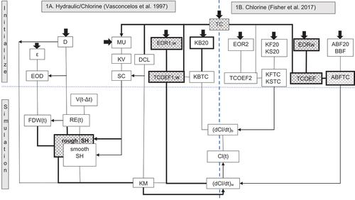
Figure 1. Relationships between temperature and hydraulic/FO chlorine variables (part 1A) and water quality (2RA/EXPBIO) in AQUASIM (part 1B) at simulation time t. Variables and parameters are defined in the Nomenclature section. User-defined inputs are shown as broad arrows. Pathway directions are downwards and to the right unless indicated by arrowheads. Variables and pathways added in this study are shown bold/hatched.

Flow and chlorine concentration in single pipes of the same diameter and roughness as in section 2.6 were simulated using the combined FO/EXPBIO model in AQUASIM. A pipe length (5000 m) similar to the entire Mirrabooka pipeline was used, and flow was set to achieve a similar retention time of 5 h. The same KB value was used in the Mirrabooka FO model, but the value of EOR was increased to 5000 K, comparable with those estimated by earlier researchers (Kiéné, Lu, and Lévi 1998; Powell et al. 2000), which are still lower than those derived for some Australian waters.

The magnification/attenuation factor TCOEF (Equation 6(6) $\mathrm{T}\mathrm{C}\mathrm{O}\mathrm{E}\mathrm{F}=exp\left[\mathrm{E}\mathrm{O}\mathrm{R}\ast \left(\mathrm{T}\mathrm{C}-20\right)/\left(20+273\right)/\left(\mathrm{T}\mathrm{C}+273\right)\right]$(6) ) was calculated from EOR and TC and applied to KB (as in Eq. 4(4) ${\left(\mathrm{d}\mathrm{C}\mathrm{l}/\mathrm{d}\mathrm{t}\right)}_{\mathrm{b}}=\hspace{0.17em}\mathrm{K}\mathrm{B}\mathrm{T}\mathrm{C}\ast \mathrm{C}\mathrm{l}$(4) ) to obtain the coefficient values for the simulations of bulk decay with the FO model at 10 and 30°C.

The EXPBIO parameters ABF20 and BBF shown in Figure 1b describe the increase in wall reactivity with decrease in chlorine concentration along the system. ABF20 is the reactivity at zero chlorine and 20°C. As with the KW0 and KW1 of Vasconcelos et al. (1997), ABFTC is likely to be temperature dependent through an Arrhenius relationship Equations. (5(5) $\mathrm{K}\mathrm{B}\mathrm{T}\mathrm{C}=\mathrm{K}\mathrm{B}20\ast \mathrm{T}\mathrm{C}\mathrm{O}\mathrm{E}\mathrm{F}$(5) ,6(6) $\mathrm{T}\mathrm{C}\mathrm{O}\mathrm{E}\mathrm{F}=exp\left[\mathrm{E}\mathrm{O}\mathrm{R}\ast \left(\mathrm{T}\mathrm{C}-20\right)/\left(20+273\right)/\left(\mathrm{T}\mathrm{C}+273\right)\right]$(6) ) with a value of EOR different from the bulk-reaction value. However, this EOR can only be evaluated from in-system data (unlike the value for bulk reactions). In the absence of such data, EOR for the wall reaction is assumed to be the same as that for the bulk reactions. This gives a conservative estimate of the temperature effect, compared with EOR values (~8000 K) measured in environmental biological assemblages (Pietikäinen, Pettersson, and Båäth 2005).

The third version of EXPBIO (EXBRUF) for rough pipes was adopted to demonstrate the effects of seasonal temperature on chlorine profiles which largely vary between the limits of 10°C and 30°C. EOR for Mirrabooka treated water (~1000 K) is small compared with most treated waters (Kiéné, Lu, and Lévi 1998; Powell et al. 2000), possibly because it is sourced from deep aquifers. A more typical value of 5000 K was adopted for both bulk and wall-reactions for this demonstration.

3. Results and discussion

3.1. Mirrabooka bulk-decay model

To best fit the summer Mirrabooka decay-test data, the optimal values of KB20 and EOR of the variable-temperature FO bulk-decay model were found within AQUASIM to be 0.1103 h⁻¹ and 806 K respectively (Table 1). The EOR value is similar to that derived for the 2RA bulk-reaction model (1300 K) but much lower than those derived for other waters (>5000 K) by researchers cited in the Introduction and for the slow reactants of Monteiro et al. (2015). This is possibly due to the source water being an artesian/groundwater mixture. The close agreement of the Mirrabooka decay-test data and the FO model’s chlorine predictions is shown in Figure S3.

Chlorine was also predicted at the four downstream measurement stations along the Mirrabooka pipeline from the AQUASIM system model, assuming either the FO or 2RA bulk-reaction model. Differences of ≤0.01 mg/L were obtained at all stations, showing that differences in all later modelling results are not due to differences in the bulk-reaction model used.

These predictions correspond to the concentrations that would prevail in-system if there were no reactions of chlorine with pipe walls; i.e. only ‘true’ bulk decay occurred. This enables determination of ‘true’ wall-reaction, rather than selecting FO or ZO wall-decay coefficients to simply ‘close the gap’ between inaccurate first-order or single-reactant bulk-decay predictions and in-system measurements.

3.2. Chlorine profiles from FO (bulk) with ZO/FO (wall) models of Mirrabooka pipeline

The average chlorine concentrations along the Mirrabooka pipeline from Jan03 that were used for wall-reaction parameter optimization in AQUASIM are shown in Figure 2a. The combined model variants and their respective optimized parameter values, which were developed within AQUASIM and run to produce the results in Sections 3.2 to 3.4, are given in Table 1.

Figure 2. Chlorine concentrations along the Mirrabooka pipeline in Jan03 (triangles) and corresponding predictions from a: FO bulk model (dotted) and in combination with ZO (dashed) and FO (unequal dashed) wall models and b: FO bulk model (dotted) and in combination with EXPBIO – rough KM (solid); EXBDYN – smooth KM (long dash), and EXBRUF – fitted KM (short dash) wall models. Model parameter values are given in Table 1.

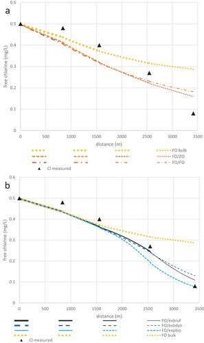
For the combined FO/ZO model, the optimal value of KW0 was found to be 0.0409 mg/dm²/h, whereas the optimised KW1 value for the FO/FO model was 0.182 dm/h. Corresponding (best-fit) chlorine profiles obtained using these optimised bulk and wall-decay coefficient values are also shown in Figure 2a.

The predictions from the bulk-only (FO) decay model lie slightly below the data at stations M2 and M3, but well within measurement error. This underprediction is worse in the results from either of the combined FO/ZO and FO/FO models because their predicted wall decay is greatest at the upstream end. This underprediction is balanced by the overprediction that increases below station M4. Increasing the value of KW in either model only makes the error greater at M2 and M3 than the improvement at M5. Clearly, the functional form of the ZO and FO wall models is not conceptually adequate to describe the variation in chlorine concentrations in this real system. Their form is similarly inadequate for prediction in any other system in which the wall-decay rate is negligible upstream, then increases with decreasing chlorine concentration downstream, as observed in another two Australian systems and confirmed by Monteiro, Caneiro and Covas (2020) in a major Portuguese pipeline.

3.3. Chlorine profiles from FO (bulk)/EXPBIO (wall) models of Mirrabooka pipeline in Jan03

Predictions from the combined FO/EXPBIO model in Jan03, using parameter values derived from these quantified data, are shown in Figure 2b with the measured chlorine data and FO bulk model predictions. In contrast to the combined models using a ZO or FO wall-reaction, these (and all later predictions using EXPBIO) show negligible reduction below the bulk-only predictions at stations M2 and M3.

The EXPBIO parameters included a fitted constant for KM, rather than the pipe-specific calculation of Vasconcelos et al. (1997). Predictions of chlorine from this FO/EXPBIO model (not previously presented) are shown in Figure 2b. The excellent prediction of chlorine at M5 was obtained at the expense of a poorer prediction at M4. However, the overall chlorine profile still has a (slightly) negative sigmoidal shape, just as the FO/ZO and FO/FO models produce, rather than the apparent convex-upward shape of the data. The combined FO/EXBDYN model, which instead included the smooth-pipe KM calculation, considerably improved the prediction at M4 at the expense of the M5 prediction (Figure 2b). However, the calculated KM values were all substantially less than the fitted value of 0.8 dm/h in the 2RA/EXPBIO model. In contrast, including the rough-pipe KM calculation in the combined FO/EXBRUF model increased the KM values by about 40%, so that KM in the downstream pipe (0.73 dm/h) almost equalled the fitted value. The corresponding chlorine profile (Figure 2b) also considerably improved the prediction at M5 while maintaining accuracy at M4. However, it is still sigmoidal in shape, suggesting that the measured profile may appear to be convex upward only because there are insufficient downstream measurement stations. Differences between measured and predicted concentrations in both chlorine profiles were within experimental error at all four stations (M2-M5), but the fit and the overall shape of the rough-pipe chlorine profile are superior.

3.4. Predicted chlorine profiles for Mirrabooka pipeline in Mar03 and Feb04

Chlorine profiles predicted for the Mar03 data period by the FO (bulk) model combined with each version of the EXPBIO wall models are shown in Figure 3a. The wall-model parameters were kept identical to those from the Jan03 simulation – only the flows and temperatures (Table 1) were different. Predictions from the rough-pipe version FO/EXBRUF are better than those from smooth-pipe version FO/EXBDYN at the most downstream station M5. However, the predictions from the original FO/EXPBIO model are better still, at both stations M4 and M5. This is probably due to the parameters of Fisher, Kastl and Sathasivan (2017) being obtained from all quantified wall-decay rates for Jan03 and Mar03, whereas the EXBRUF and EXBDYN versions have been fitted to only the Jan03 chlorine data. The superior FO/EXPBIO predictions of the Mar03 chlorine data compared to those of the Jan03 data corroborates this view.

Figure 3. Chlorine concentrations along the Mirrabooka pipeline (triangles) in a: Mar03 and b: Feb04 with corresponding predictions from FO bulk model (dotted) and in combination with EXPBRUF – rough KM (solid); EXPBDYN – smooth KM (long dash), and EXBIO – fitted KM (short dash) wall models. Model parameter values are as for Jan03 (Figure 2b).

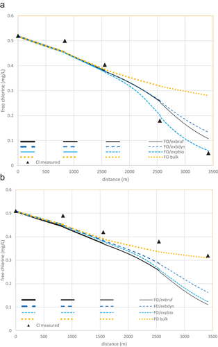
Figure 3b shows similar chlorine data for Feb04 and their prediction from the three FO/EXPBIO model combinations. The FO bulk-decay model alone was the best predictor, as there was no quantifiable wall-reaction. The 13% increase in flow entering the pipeline (and consequent decreased reaction time) in Mar03 is already accounted for in the simulation results. A possible explanation for the underprediction from all models is that there was a mains cleaning program downstream of the pipeline just before the Feb04 data period. This would have drawn much higher flow through the pipeline, possibly removing much of the active biofilm that existed during the calibration period (Jan03).

3.5. Significance of effects of temperature in single smooth and rough pipes

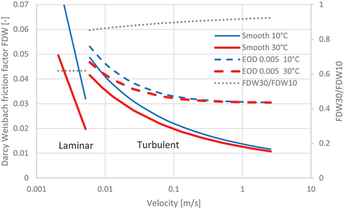
A substantial difference in the Darcy-Weisbach friction factor (FDW) was obtained from assuming a smooth or a rough pipe of 0.5 m diameter and relative roughness (EOD) of zero or 0.005 respectively at constant temperature (Figure 4). FDW-rough varies from 13% greater than FDW-smooth at RE = 2300 to 254% greater at a velocity of 1 m/s.

Figure 4. Darcy-Weisbach friction factor as a function of velocity in 0.5 m diameter pipe: solid lines – smooth pipe, turbulent and laminar flow; dashed lines – rough pipe (relative roughness 0.005), turbulent flow; thin lines − 10°C; thick lines 30°C.

The effect of temperature on hydraulic flow was evaluated by comparing FDW calculated from Eq. 11(11) $\mathrm{S}\mathrm{H}=\left(\mathrm{F}\mathrm{D}\mathrm{W}/8\right)\ast \left(\mathrm{R}\mathrm{E}-1000\right)\ast \mathrm{S}\mathrm{C}/[1+12.7\ast \left(\mathrm{F}\mathrm{D}\mathrm{W}/8\right){ }^{{\hspace{0.17em}}_{\hspace{0.17em}}^{}\wedge }0.5\ast (\mathrm{S}\mathrm{C}{ }^{{\hspace{0.17em}}_{\hspace{0.17em}}^{}\wedge }0.667-1)]$(11) at 10°C and 30°C at the same velocity, rather than the same RE, because temperature affects RE directly. Pairs of these values of FDW are shown in Figure 4 for the same smooth and rough pipes.

Figure 4 also shows that FDW30 is only 62% of FDW10 in the laminar flow region. However, this ratio increases to 86% at the low end of the turbulent region (RE ~ 2300) in a smooth pipe and increases to 91% at a velocity of 1 m/s.

The effect of the change in FDW over this temperature range on either flow or chlorine concentration is not possible to judge as it depends heavily on the location of the pipe and head/flows in the network. However, it is important to capture this effect in the hydraulic calculations before passing FDW to any calculation of the mass transfer coefficient (KM).

The effect of temperature on KM was similarly evaluated by calculating KM at 10°C and 30°C at the same velocity over the turbulent range (RE > 2300). The results are shown in Figure 5. In the same rough pipe, KM30 was 250% greater than KM10 at low RE and over 200% greater for RE above 5000.

Figure 5. Mass transfer coefficient (KM) as a function of velocity at 10°C and 30°C in a smooth (_S) and rough pipe (diameter 0.5 m, relative roughness 0.005).

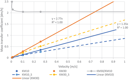
This difference over the whole turbulent velocity range is sufficient to warrant inclusion of temperature in the computation of KM for use in any wall-reaction model.

From Figure 5, at a velocity of 0.51 m/s, KM is 0.69 dm/h at 10°C and 0.90 dm/h at 30°C. These values bracket the value for KM of 0.8 dm/h derived by Fisher, Kastl and Sathasivan (2017) for the Mirrabooka pipeline at 22.6°C, thus enabling the temperature effect on KM to be included in the current simulations at 10 and 30°C.

Figure 6 shows the simulated chlorine concentration profile along the rough pipe at 10 and 30°C. The ‘bulk only’ concentrations are those obtained from the FO model alone, i.e. as if the pipe walls are inert so that there is no wall reaction at all. The ‘bulk with expbio wall’ profile is from the combined FO/EXPBIO model. At 10°C, there is almost no decrease in chlorine due to wall reaction.

Figure 6. Simulated chlorine concentration in a rough pipe of 0.5 m diameter at 10 and 30°C.

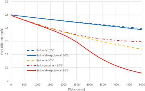
In contrast, at 30°C, the longitudinal chlorine profile has the same sigmoidal shape and lies well below the ‘bulk only’ profile. It is important to note that the ‘bulk only’ profile does not give the correct contribution to the combined model profile because the chlorine concentration at any downstream location is lower in the combined case (due to the decrease caused by the wall reaction). Consequently, the bulk reaction rate is lower than in the combined case. The true contribution due to the bulk reaction is obtained by tracking the decrease due to bulk reaction in the combined model simulation. This is shown as the ‘bulk component’ in Figure 6. As expected, it is less than that obtained from the ‘bulk only’ simulation.

The major contribution to the substantial differences in chlorine profiles must therefore come from differences in wall-reaction rates. These rates increase with temperature due to the increase in KM (Figure 5) and the non-linear increase in biofilm activity (ABFTC). The corresponding differences between chlorine profiles are likely to be even greater in pipes of smaller diameter, which is often as little as 0.1 m in distribution systems.

The dramatic differences in the chlorine profiles from simulations at 10 and 30°C strongly justify the inclusion of the temperature effect in both chlorine bulk and wall reaction models within a multi-species simulation environment such as AQUASIM or EPANET-MSX.

3.6. Effects of temperature from combined FO/EXBRUF model of Mirrabooka pipeline

Bulk reactions in water supplying the Mirrabooka pipeline have a low temperature sensitivity (EOR ~1000K) compared with most other waters (EOR >5000K – see Introduction). Consequently, the modelling comparison of the overall effects of temperature on Mirrabooka chlorine profiles presented in this Section adopted a more typical value of 5000 K. Figure 7 shows the differences in chlorine profiles simulated at 10, 20 and 30°C with the rough-pipe (ε = 0.0025 m) version FO/EXBRUF. The 20°C profile is only slightly higher than the corresponding one (and measured data) of Figure 2, due to the higher temperature of the latter simulation (22.6°C). In the absence of any better information, the same temperature sensitivity has been assumed for the biofilm reactivity parameter ABFTC as that assumed for KBTC in the FO bulk reaction (EOR = 5000 K). Parameter BBF characterises the decrease in reactivity as chlorine increases from zero. This decrease automatically scales with ABF20, so that BBF may be less temperature-sensitive. Further in-system data is needed to confirm whether it is a significant influence.

Figure 7. Simulated chlorine profiles along the Mirrabooka pipeline Jan03. Chlorine profiles simulated at 10, 20 and 30°C with the combined FO/EXBRUF model including temperature sensitivity of parameters KBTC and ABFTC (EOR = 5000 K).

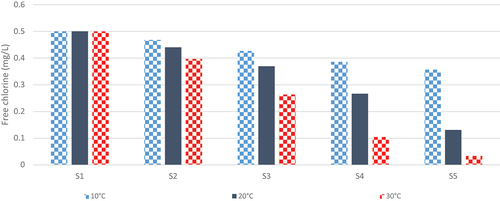
Clearly, temperature variation would affect the wall reaction far more than the bulk reaction in such a steady flow-dominated system, indicated by the substantial increasing differences at the last three stations. Consequently, it appears to be extremely important to include the temperature effects on both bulk and wall-reaction model parameters when deriving disinfection strategies for different seasonal conditions from simulations of distribution systems.

3.7. Effect of simulation timescale

It could be argued that the biofilm development along the pipeline is in equilibrium with the average chlorine concentrations experienced on a timescale of weeks rather than that of the simulations (usually 24 h). The equilibrium biofilm development in the same pipeline, but with different bulk and wall EOR values, would be different from that in the monitored pipeline and hence the wall reaction would be different. Consequently, the simulation results in Figure 7 can only be regarded as indicative of the importance of temperature differences in any particular real system.

For the same reason, wall-reaction models such as the ZO, FO or EXPBIO models, which are all functions of bulk chlorine concentration, would not necessarily give accurate predictions of chlorine concentration under realistic diurnal variations in demand, which can be readily implemented in widely used system modelling software such as EPANET and EPANET-MSX. To realistically simulate such dynamic changes, models that represent the biofilm as a separate species on the wall are required (e.g. Jegatheesan et al. 2000). Model validation would involve biofilm measurement techniques applied in-system, along with chlorine monitoring, which would require major and sustained resources.

4. Conclusions

• The widely used zero- and first-order wall-reaction models conceptually contradict the initially zero, then increasing, wall-decay rate associated with decreasing bulk chlorine concentration observed in real pipelines. So too is the ‘Equivalent Diameter’ wall-reaction model. They are all therefore structurally invalid.

• In contrast, the EXPBIO wall-reaction model is conceptually consistent with such real pipeline data. To make it generally applicable to pipe networks, new versions were developed to calculate the mass transfer coefficient in each pipe. This also improves model efficiency by reducing the number of fitted parameters to two.

• Both the smooth-pipe version (EXBDYN) and the rough-pipe version (EXBRUF) were formally validated against chlorine concentration data observed in the Mirrabooka pipeline on three different occasions several months apart.

• Although the EXBRUF predictions were marginally superior to those from EXBDYN at low concentrations, greater superiority is expected in parts of a network with smaller pipe diameters.

• The effect of pipe roughness is sufficiently large to warrant its inclusion in the computation of the mass-transfer coefficient in any wall-reaction process model, particularly at higher velocities.

• Within the general operating range of 10-30°C, the Darcy-Weisbach friction factor (FDW) is substantially lower at higher temperature in the laminar flow range, but the difference decreases with increasing velocity in the turbulent range.

• In contrast, the mass transfer coefficient (KM) for chlorine increases substantially with temperature and increasing velocity in the turbulent range.

• These two major temperature effects are sufficient to warrant their inclusion in hydraulic system simulation, particularly when involved in searching for improved disinfection strategies in different seasons.

• Increasing temperature over the same operating range has much greater direct effects on rates of both bulk and wall reactions with chlorine. In general, these can be accurately and efficiently accounted for by implementing a combined 2RA (bulk)/EXPBIO (wall) chlorine-reaction model within a multi-species simulation environment.

• Simulation of chlorine concentrations in a real multi-segment pipeline highlighted the major effect that temperature can have in flow-dominated systems. Temperature effects are expected to be greater in systems containing tanks due to their greater retention time.

• The combined 2RA/EXPBRUF model provides a robust description of chlorine decay in a distribution system, simulating observed behaviour initially driven by the bulk decay and later accelerated by wall decay when chlorine concentration is low enough to allow biofilm growth.

5. Data and software availability

Data from the Mirrabooka pipeline used in the formal validation (and from pipelines in two other distribution systems) are given in the Supplementary Material of Fisher, Kastl and Sathasivan (2017). Dissemination of these data requires permission from the respective water utilities. Optimal parameter values for the temperature-affected bulk-reaction model were derived using the AQUASIM batch-reactor software (Reichert 1994). The widely used first- and second-order wall-reaction models described by Vasconcelos et al. (1997) for smooth pipes are fully documented in the EPANET 2 software user manual (Rossman 2000). These models; the EXPBIO wall-reaction model, and the equivalent wall-reaction models for rough pipes proposed in this paper, were programmed in the AQUASIM advective-reactive system software (Reichert 1994) to provide a common basis for comparison in either single or contiguous pipes specified in this paper.

Nomenclature

Table

Symbol	Parameter/Variable	Unit
TC	Temperature	°C
MU	Dynamic viscosity	Pa s
RHO	Density	kg/m^3
KV	Kinematic viscosity	m^2/s
D	Pipe diameter	m
V	Pipe velocity	m/s
RE	Reynolds Number	-
EOD	Relative roughness (ε/D)	-
HL	Head loss along pipe	m
L	Pipe length	m
G	Gravitational acceleration	m/s^2
FDW	Darcy-Weisbach friction factor	-
DCL	Diffusivity of chlorine in water	m^2/s
SC	Schmidt Number (KV/DCL)	-
SH	Sherwood Number	-
KM	Mass transfer coefficient	m/s or dm/h*
ZO, FO and SO	Zero, first and second order (bilinear) reaction kinetics
KBTC	FO bulk decay-rate coefficient at TC	/h
EOR	Bulk reaction activation energy (E)/gas constant (R)	K
TCOEF	Temperature amplification coefficient	-
Cl(t)	Chlorine concentration in bulk water (at time t h)	mg/L
(dCl/dt)b	Rate of reaction of chlorine in bulk water	mg/L/h
KW0	Zero-order wall-reaction coefficient	mg/dm^2/h
KW1	First-order wall-reaction coefficient	dm/h
(dCl/dt)w or WRR	Surficial rate of reaction of chlorine with wall (biofilm)	mg/dm^2/h
2RA	Dynamic two-reactant second-order (bilinear) model of chlorine reactions in bulk water
KFTC	SO fast bulk reaction-rate coefficient at TC	L/mg/h
KSTC	SO slow bulk reaction-rate coefficient at TC	L/mg/h
F	Fast reactant concentration in bulk water	mg Cl-equiv/L
S	Slow reactant concentration in bulk water	mg Cl-equiv/L
EXPBIO, EXBDYN & EXBRUF	Biofilm-mediated wall reaction models
ABFTC	Biofilm activity at zero chlorine and temperature TC	dm/h
BBF	Biofilm activity decrease with chlorine increase	L/h
AQUASIM	System modelling/parameter optimization software

*for compatibility with units involving volume [L] in chlorine-reaction models In all equations, the × symbol denotes multiplication (there are no vectors involved in this paper).

Acknowledgements

Laboratory and field data from the Mirrabooka system were obtained by Western Australia Water Corporation, under the direction of the authors, as a contribution to the research program of the Australian Cooperative Research Centre for Water Quality and Treatment. Author contributions: IF conceptualized the research; IF and GK curated the data and devised the methods; IF administered the project, developed models in AQUASIM, conducted validation and visualisation of results and wrote the original draft. GK and AS reviewed and edited several drafts and IF produced the final version.

Disclosure statement

No potential conflict of interest was reported by the author(s).

Supplemental data

Supplemental data for this article can be accessed https://doi.org/10.1080/1573062X.2023.2241437.

Correction Statement

This article has been corrected with minor changes. These changes do not impact the academic content of the article.

Additional information

Funding

This research did not receive any specific grant from funding agencies in the public, commercial, or not-for-profit sectors.

References

- Fisher, I., G. Kastl, and A. Sathasivan. 2012. “A Suitable Model of Combined Effects of Temperature and Initial Condition on Chlorine Bulk Decay in Water Distribution Systems.” Water Research 46 (10): 3293–3303. https://doi.org/10.1016/j.watres.2012.03.017.
- Fisher, I., G. Kastl, and A. Sathasivan. 2016. “A Comprehensive Bulk Chlorine Decay Model for Simulating Residuals in Distribution Systems.” Urban Water Journal 14 (4): 361–368. https://doi.org/10.1080/1573062X.2016.1148180.
- Fisher, I., G. Kastl, and A. Sathasivan. 2017. “New Model of Chlorine-Wall Reaction for Simulating Chlorine Concentration in Drinking Water Distribution Systems.” Water Research 125:427–437. https://doi.org/10.1016/j.watres.2017.08.066.
- Hallam, N., J. West, C. Forster, and J. Simms. 2001. “The Potential for Biofilm Growth in Water Distribution Systems.” Water Research 35 (17): 4063–4071. https://doi.org/10.1016/S0043-1354(01)00248-2.
- Jegatheesan, V., G. Kastl, M. Angles, J. Chandy, and I. Fisher. 2000. “Modelling Biofilm Growth and Disinfectant Decay in Drinking Water.” Water Science and Technology 41 (4–5): 339–345. https://doi.org/10.2166/wst.2000.0464.
- Kastl, G., I. Fisher, J. Chandy, V. Jegatheesan, and K. Clarkson. 2003. “Prediction of Chlorine and Trihalomethanes Concentration Profile in Bulk Drinking Water Distribution Systems from Laboratory Data.” Water Science and Technology: Water Supply 3 (1–2): 239–246. https://doi.org/10.2166/ws.2003.0110.
- Kiéné, L., W. Lu, and Y. Lévi. 1998. “Relative Importance of the Phenomena Responsible for Chlorine Decay in Drinking Water Distribution Systems.” Water Science and Technology 38 (6): 219–227. https://doi.org/10.2166/wst.1998.0255.
- Monteiro, L., J. Caneiro, and D. Covas. 2020. “Modelling Chlorine Wall Decay in a Full-Scale Supply System.” Urban Water Journal 17 (8): 754–762. https://doi.org/10.1080/1573062X.2020.1804595.
- Monteiro, L., R. Viegas, D. Covas, and J. Menaia. 2015. “Modelling Chlorine Residual Decay as Influenced by Temperature.” Water and Environment Journal 29 (3): 331–337. https://doi.org/10.1111/wej.12122.
- Notter, R., and C. Sleicher. 1971. “The Eddy Diffusivity in the Turbulent Boundary Layer Near a Wall.” Chemical Engineering Science 26 (1): 161–171. https://doi.org/10.1016/0009-2509(71)86088-8.
- Pietikäinen, J., M. Pettersson, and E. Båäth. 2005. “Comparison of Temperature Effects on Soil Respiration and Bacterial and Fungal Growth Rates.” FEMS Microbiology Ecology 52 (1): 49–58. https://doi.org/10.1016/j.femsec.2004.10.002.
- Powell, J., N. Hallam, J. West, C. Forster, and J. Simms. 2000. “Factors Which Control Bulk Chlorine Decay Rates.” Water Research 34 (1): 117–126. https://doi.org/10.1016/S0043-1354(99)00097-4.
- Reichert, P. 1994. “AQUASIM – a Tool for Simulation and Data Analysis of Aquatic Systems.” Water Science and Technology 30 (2): 21–30. https://doi.org/10.2166/wst.1994.0025.
- Rossman, L. 2000. EPANET2 Users Manual. Cincinnati, Ohio: US EPA.
- Swamee, P., and A. Jain. 1976. “Explicit Equations for Pipe-Flow Problems.” Journal of the Hydraulics Division 102 (5): 657–664. https://doi.org/10.1061/JYCEAJ.0004542.
- Taler, D., J. Taler, J. Taler, B. Węglowski, and T. Sobota. 2017. “Simple Heat Transfer Correlations for Turbulent Tube Flows.” E3S Web of Conferences 13:02008. https://doi.org/10.1051/e3sconf/20171302008.
- Vasconcelos, J., L. Rossman, W. Grayman, P. Boulos, and R. Clark. 1997. “Kinetics of Chlorine Decay.” Journal - American Water Works Association 89 (7): 54–65. https://doi.org/10.1002/j.1551-8833.1997.tb08259.x.