Optimal opportunistic tamping scheduling for railway track geometry

Abstract

This study has been dedicated to the optimization of opportunistic tamping scheduling. The aim of this study has been to schedule tamping activities in such a way that the total maintenance costs and the number of unplanned tamping activities are minimized. To achieve this, the track geometry tamping scheduling problem was defined and formulated as a mixed integer linear programming (MILP) model and a genetic algorithm was used to solve the problem. Both the standard deviation of the longitudinal level and the extreme values of isolated defects were used to characterize the track geometry quality and to plan maintenance activities. The performance of the proposed model was tested on data collected from the Main Western Line in Sweden. The results show that different scenarios for controlling and managing isolated defects will result in optimal scheduling plan. It is also found that to achieve more realistic results, the speed of the tamping machine and the unused life of the track sections should be considered in the model. Moreover, the results show that prediction of geometry condition without considering the destructive effect of tamping will lead to an underestimation of the maintenance needs by 2%.

Keywords:

• Degradation
• genetic algorithms
• logistic regression
• Maintenance
• optimal scheduling
• railway tracks
• tamping

1. Introduction

The railway track geometry is subjected to continuous degradation over time and deviates from the designed vertical and horizontal alignments due to different factors, e.g., repetitive dynamic track loads and environmental conditions. Maintenance is required to control or prevent the process of degradation and to keep the track in a safe and functional state. The track quality is quantified through a set of track geometry parameters, e.g., the longitudinal level, alignment, cant, gauge, and twist. According to EN 13848-5 (2008), there are three indicators that represent the track geometry condition for sections of a specific length, i.e. the standard deviation, the mean value and the extreme value of isolated defects.

Whenever the track geometry indicators exceed some predetermined limits, maintenance actions, e.g., tamping, will be performed to remedy a degraded track geometry. Tamping can be either corrective or preventive. Corrective tamping is unscheduled and is generally carried out on a short length of track, mainly using lightweight machines. Preventive tamping, on the other hand, is planned and scheduled and is cheaper than corrective tamping because it is pre-planned and does not affect the service operation. Generally, the standard deviation of geometry parameters is used to assess the overall condition of a track section and to plan for preventive tamping activities (UIC, 2008). However, since the standard deviation aggregates the track geometry measurements over a track section, it may not provide complete information regarding the occurrence of severe isolated defects (Soleimanmeigouni, Ahmadi, Nissen, & Xiao, 2020). Isolated defects significantly influence the running behaviour of trains and are the main reason for conducting corrective tamping activities (Khajehei, Ahmadi, Soleimanmeigouni, & Nissen, 2019). Therefore, both these indicators should be considered in geometry evaluation to have a better picture of the track geometry condition and to draw up an effective and efficient tamping schedule.

Since a railway track is a linear and non-redundant system, the availability and safety of a track line depend directly on the reliability and quality of all the individual track sections. A proper tamping scheduling regime is crucial to maintain the track geometry quality on an acceptable level, and affects positively the track availability and capacity. In order to conduct tamping activities in a way that does not disrupt the normal traffic, infrastructure managers (IMs) set maintenance windows on a regular basis. In an upcoming available maintenance window, a challenge is to determine which track sections must be tamped to keep the track quality on a desirable level in consideration of practical constraints, e.g. resource limitations.

As a best practice within railway maintenance planning and scheduling, the track sections can be grouped for tamping actions, enabling the application of opportunistic maintenance (OM) scheduling, to benefit the system reliability and availability and reduce the maintenance cost. OM scheduling is one of the most important issues in railway engineering as a maintenance plan that does not consider opportunistic tamping is usually impractical. With regard to maintenance of the track geometry, the normally limited amount of maintenance equipment and the normally limited track possession time for tamping highlight the importance of applying OM by grouping track sections for tamping. OM is a strategy for performing more tamping than necessary on track sections, within the assigned possession time and in the available maintenance window, to reduce the need for tamping in the near future.

The benefits of performing OM on track sections are based on the existence of different kinds of dependence. Three types of dependence among track sections can be considered, namely stochastic dependence, structural dependence and economic dependence. The existence of stochastic dependence (Pham, 2003; Thomas, 1986; Castanier, Grall, & Bérenguer, 2005) means that the degradation in one track section may influence the degradation of other track sections. This dependence was proved by Andrade & Teixeira (2011) and Soleimanmeigouni, Ahmadi, and Kumar (2018). They confirmed that there is a correlation between the degradation of adjacent track sections and that determining the dependence between different track sections provides an opportunity to group the track sections better for tamping. Structural dependence means that performing tamping on a track section may affect the state of other track sections due to the physical interaction among track sections.

With respect to economic dependence (Wang, 2002; Gustavsson, 2015; Thomas, 1986; Nicolai & Dekker, 2008), once a tamping activity has been triggered, the machines and logistics available for the tamping of that track section can be used for the tamping of other track sections and the maintenance cost can thereby be reduced. In order to derive the advantages of the OM policy, which involves postponing tamping actions on track sections or performing them earlier, it is necessary to analyse the scheduling problem from the perspective of the future condition of the track. Therefore, generally the tamping scheduling problem is defined for a finite time horizon of three to five years. It must be noted that, after conducting tamping in a maintenance window, it is necessary to re-schedule the tamping activities with the new available dataset.

Several research studies have been conducted on the scheduling of preventive tamping activities. Vale, Ribeiro, and Calçada (2012) considered the standard deviation of the longitudinal level (SDLL) as the track quality indicator and presented a mathematical maintenance model which provides a tamping schedule that minimizes the total number of tamping actions. Gustavsson (2015) proposed a mixed integer linear programming (MILP) model for tamping scheduling to minimize the cost of tamping in the given planning horizon by considering the SDLL as the track quality indicator. In this study, Gustavsson considered OM from the perspective of economic dependence by considering a setup cost in the model. The degradation model presented by this author is a combination of a linear and an exponential model in the sense that he added a parameter to the degradation model which would make it possible to control the rate of degradation.

Wen, Li, and Salling (2016) considered the SDLL as the quality indicator and tried to determine when and where to perform tamping to minimize the net percent cost of preventive tamping in the given time horizon. These authors determined the OM schedule by considering economic dependence in their cost model. They formulated the problem as a MILP model and solved it using CPLEX for a period of 3.5 years. Budai, Huisman, and Dekker (2006), Budai-Balke, Dekker, and Kaymak (2009) and Macedo, Benmansour, Artiba, Mladenović, and Urošević (2017) clustered routine maintenance activities and projects with the aim of minimizing the track possession and maintenance costs. Pargar, Kauppila, and Kujala (2017) scheduled the preventive maintenance and renewal of a multi-component system by using a technique for grouping and balancing maintenance actions to minimize the maintenance and renewal costs. In addition, Peralta et al. (2018) developed a model for optimizing the tamping and renewal activities in the short and long term with the aim of minimizing the maintenance cost and delay. These authors used the SDLL as the quality indicator and applied an exponential model to predict the future condition of the track.

Dao, Basten, and Hartmann (2018) proposed a model for the optimal scheduling of railway maintenance and renewal. Their aim was to minimize the total cost of railway maintenance over the planning horizon. They also considered the limitation of the track possession time for maintenance and renewal work. In another study, Lee, Choi, Kim, and Hwang (2018) proposed a model for minimizing the number of tamping and renewal interventions and the maintenance costs simultaneously. In this study, the SDLL was considered as the quality indicator and a linear model was used to predict the degradation of the track geometry in the future. In the degradation model, the degradation rate is a function of the number of tamping actions and the tamping effectiveness is decreased by increasing the number of tamping actions.

In addition, there exist a small number of studies that have considered the probability of the occurrence of isolated defects as well. He, Li, Bhattacharjya, Parikh, and Hampapur (2015) developed a model for predicting the degradation process of various geo-defects. Later on, they proposed a model for assessing the risk of derailment and, finally, proposed an analytical framework for making optimal decisions regarding the rectification of geo-defects. Sharma, Cui, He, Mohammadi, and Li (2018) developed a Markov decision process (MDP) model to make optimal decisions regarding preventive and corrective tamping activities on each inspection occasion. The aim of these authors was to harmonize maintenance decision making to minimize the total maintenance costs.

Searching the relevant literature, it can be seen that an obvious challenge which needs to be overcome is to provide a scheduling plan which, in addition to minimizing the maintenance cost and maintaining the overall geometry quality, also minimizes the number of corrective maintenance actions. Another challenge to be met for the achievement of an efficient tamping schedule is the creation of a reliable model for accurate prediction of the track geometry evolution. Therefore, one needs to consider the effect of tamping on the degradation pattern. Tamping interventions have two main effects on the track geometry condition, i.e. a change in the degradation rate and a change in the degradation level. Tamping is an imperfect maintenance intervention and the track geometry condition after tamping will not have been improved to an ‘as-good-as-new’ condition. Hence, considering the effect of tamping on the degradation pattern is of importance for estimating the maintenance needs to achieve an effective scheduling. To this end, the present study was undertaken to find the optimal tamping schedule and to address the aforementioned issues.

This study presents an optimization model for the problem of preventive tamping scheduling using an OM approach. The aim is to propose an OM-based tamping schedule which minimizes the total maintenance costs and the number of corrective tamping actions due to the occurrence of isolated defects in a given time horizon. In order to represent the geometry condition and schedule tamping actions, the SDLL and the extreme values of isolated defects of the longitudinal level, alignment and twist are used as track quality indicators. An exponential function is used to model the track geometry degradation. In addition, binary logistic regression is used to estimate the probability of the occurrence of severe isolated defects. In order to achieve an optimal schedule for preventive tamping, the problem is formulated as a MILP model. OM has been considered in the model in the form of economic and structural dependence. Regarding economic dependence, it is considered that a fixed cost is incurred whenever a tamping intervention is carried out on a track section in a maintenance window. The fixed cost concerns the available maintenance equipment and crew and, therefore, creates the opportunity to perform more tamping than necessary (Gustavsson, 2015). Concerning structural dependence, a constraint is proposed which stipulates the performance of tamping on a track section located between two track sections that need to be tamped.

It has been proven that the preventive tamping scheduling problem is a non-deterministic polynomial-time hard (NP-hard) problem (Peralta et al., 2018; Zhang, Andrews, & Wang, 2013). In practice, the global optimal solution cannot be computed in a feasible length of time. Therefore, it is important to develop an algorithm to find a near-optimal solution to the problem (Peralta et al., 2018). To find the optimal solution for the formulated scheduling problem in this study, a genetic algorithm (GA) is used, which is one of the most popular metaheuristic algorithms for solving NP-hard problems. In order to test the proposed model, a case study was performed on data collected from the Main Western Line in Sweden.

The rest of this paper is organized as follows: Section 2 provides a background on the track geometry parameters and maintenance limits. The problem of tamping scheduling is presented in Section 3. Section 4 deals firstly with the track geometry degradation and recovery models and the isolated defect model, and then provides the mathematical formulations relating to the tamping scheduling problem. Section 5 gives information regarding the method for solving the problem, while the case study is presented in Section 6. Finally, Section 7 provides the conclusions.

2. Track geometry quality and maintenance

The track geometry quality is typically quantified through track geometry parameters. There are five track geometry parameters, i.e. the cant, alignment, longitudinal level, twist and gauge. The geometry parameters are recorded by measurement cars at specific sampling intervals, usually at intervals of 25 cm, by running the cars over the railway track at a certain speed (Soleimanmeigouni, Ahmadi, & Kumar, 2018). Then the measured geometry parameters are used to develop track quality indicators. Three main indicators are used to represent the track geometry condition, i.e., the standard deviation, the mean value, and the extreme value of isolated defects (EN 13848-5, 2008). Once the track geometry indicators reach a predetermined maintenance limit, a proper maintenance action needs to be scheduled to restore the track geometry condition to an acceptable level. The European standard EN 13848-5 (2008) has determined three limits for maintenance actions, based on different permissible speeds, as follows:

• The immediate action limit (IAL) or safety limit refers to the value which, if exceeded, due to the potential risk of derailment, requires that a speed reduction or line closure be imposed before a corrective maintenance action is conducted.

• The intervention limit (IL) or corrective maintenance limit refers to the value which, if exceeded, requires that a corrective maintenance action be taken before the immediate action limit is reached.

• The alert limit (AL) or preventive maintenance limit refers to the value which, if exceeded, requires that the track geometry be analysed for the planning of future maintenance actions.

EN 13848-5 (2008) provides ALs for the standard deviation of geometry parameters and IALs, ILs and ALs for isolated defects.

In alignment with EN 13848-5 (2008), Trafikverket (the Swedish Transport Administration) has defined four main limits, namely the planning limit, the UH1 limit, the UH2 limit and the critical limit. In Trafikverket (2015), the intervention limit is expressed as a range rather than a discrete value. Track irregularities that exceed the UH1 limit must be assessed for conducting maintenance before the UH2 limit is exceeded. For track irregularities exceeding the UH2 limit, a maintenance action must be taken without unnecessary delay. Therefore, track irregularities must be corrected before the UH2 limit is reached. Table 1 shows the relations between the limits defined in EN 13848-5 (2008) and those defined in Trafikverket (2015). Based on the defined limits, geometry defects can be classified according to their severity into three groups, i.e., UH1, UH2 and critical defects. UH1, UH2 and critical defects occur when track irregularities exceed the UH1, UH2 and critical limits, respectively. An example of a UH2 defect is shown in Figure 1.

Figure 1. Example of a UH2 defect of the longitudinal level.

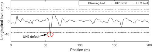
Table 1. Maintenance limits defined in the European standard EN 13848–5 (2008) and in Trafikverket (2015).

EN 13848-5 limits	Trafikverket’s limits
Alert limit	Planning limit
Intervention limit	UH1 limit (lower bound for corrective maintenance)
	UH2 limit (upper bound for corrective maintenance)
Immediate action limit	Critical limit

In this work, the SDLL has been used as the indicator for preventive tamping actions. In addition, UH2 defects of the longitudinal level, alignment and twist have been considered to represent the need for corrective tamping actions.

3. Problem description

The problem dealt with in the present study concerns the tamping scheduling of a track line consisting of$\mathrm{ }S=\left\{1,\dots ,s\dots S\right\}$ track sections with different lengths ($L_s$) in a finite time horizon T. In the given time horizon T, there exists a set of available maintenance windows$\mathrm{ }t=1,2,3,.,\mathrm{ }T,$ and each maintenance window $tϵT$ has a fixed track possession time¹ $(T^P$).

As mentioned in Section 2, the SDLL is used as the indicator for planning tamping activities. If the SDLL value of a track section $sϵS$ exceeds the planning limit (${\mathit{SDLL}}_s\ge \mathit{plan}$), then the track section will be considered as a candidate for upcoming tamping activities. Obviously, performing corrective tamping is significantly more expensive than performing preventive tamping. In addition, the occurrence of isolated defects may cause temporary speed restrictions and operational risk. Consequently, when scheduling preventive tamping, it is crucial to consider the occurrence of isolated defects, to minimize the number of corrective tamping actions between two maintenance windows. It must be noted that when an isolated defect occurs, there is a need to conduct corrective tamping actions as early as possible.

Hence, in addition to the SDLL, the isolated defects of geometry parameters are considered to represent the track geometry condition and are used to plan maintenance activities. Moreover, the probability of the occurrence of UH2 defects is used to trigger the performance of corrective tamping. If the probability of the occurrence of UH2 defects in track section $sϵS$ exceeds $\mathrm{\wp }$ ($P_s^{UH2}>\mathrm{\wp }$), then the track section must be selected for tamping in the earliest upcoming maintenance window$\mathrm{ }tϵT.$ The relationship between the probability of the occurrence of UH2 defects and the SDLL value is suitably modelled (see Section 4.2). This will be used to identify the corresponding SDLL (γ) for the occurrence of UH2 defects based on a certain value of $\mathrm{\wp }.$

By considering the SDLL and isolated defects and by using the degradation model, the maintenance actions required to keep the track quality on an acceptable level can be estimated. However, to optimize the tamping schedule, it is important to implement OM. It is assumed that in maintenance window $tϵT,$ if at least one track section needs tamping, then a fixed cost must be paid for the available tamping machines and crew. At this time, there is an opportunity to perform more tamping activities (group tamping activities) on other track sections which require tamping in the upcoming maintenance windows. The grouping of tamping activities is achieved by shifting maintenance activities to a date later or earlier than pre-planned based on different criteria.

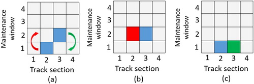
Figure 2 illustrates the shifting of tamping activities in order to group tamping operations. Figure 2a shows an ungrouped tamping schedule by assuming that track section 2 and track section 3 have reached the maintenance threshold and can be tamped in maintenance windows 1 and 2, respectively. Two illustrative scenario examples, i.e. postponing a tamping action and performing an earlier tamping action than planned are shown in Figures 2b and 2c, respectively. Shifting the tamping on track section 2 from the first maintenance window to the second maintenance window (tamping postponement) will reduce the unused life, but will increase the risk of unexpected events (see Figure 2b). On the other hand, shifting the tamping of track section 3 from the second maintenance window to the first maintenance window will reduce the risk of unexpected events, but will increase the unused life of the track section due to the earlier performance of tamping (see Figure 2c). It must be noted that in both scenarios the number of used maintenance windows is reduced, which may lead to a significant reduction of the maintenance cost and increase the track capacity.

Figure 2. (a) Preliminary tamping schedule without grouping, (b) group maintenance activities achieved by tamping postponement and (c) group maintenance activities achieved by earlier tamping.

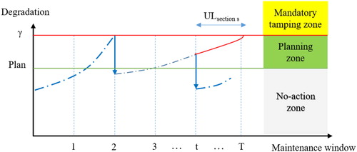
In the OM-based tamping scheduling problem, grouping tamping activities may occur for track sections with an SDLL value in the planning zone, as is shown in Figure 3, which provides a schematic description of maintenance limits and maintenance zones. Decisions regarding the shifting of tamping activities are based on the following lines of reasoning:

Figure 3. Schematic description of maintenance limits and maintenance zones.

• If the SDLL value of track section $sϵS$ in maintenance window $tϵT$ exceeds the γ limit (${\mathit{SDLL}}_s\ge \gamma$), then the track section must be tamped without any tamping postponement (see Figure 3).

• If the SDLL value of track section $sϵS$ in maintenance window $tϵT$ exceeds the planning limit and is less than the γ limit ($\mathit{plan}<{\mathit{SDLL}}_s<\gamma$), then the section will be considered for further planning. In addition, there is the possibility of either performing tamping earlier on this section or postponing the tamping activity. Moving a tamping action to an earlier maintenance window is illustrated in Figure 3 under ${UL}_{\mathit{section}s}.$ Decisions on tamping postponement or earlier tamping are taken based on a trade-off between the cost, the risk of the occurrence of UH2 defects, and the unused life of that track section due to the earlier performance of a tamping operation.

Considering the above-mentioned points, in order to optimize the tamping schedule, it is needed to answer these two questions: 1) Which maintenance window must be used to conduct tamping activities? 2) Which track sections must be tamped in the chosen maintenance window? Therefore, the two binary decision variables $x_{s,t}$ and $z_t$ have been defined as follows to address these two questions: $$x_{s,t}=\{\begin{array}{c}1\mathit{\text{ if }}\mathit{track} \mathit{section}\mathit{\text{ s is }}\mathit{tamped}\mathit{\text{ in }}\mathit{maintenance} \mathit{window} t,\hfill \\ 0 \mathit{otherwise}\hfill \end{array}$$ $$z_t=\{\begin{array}{c}1\mathit{\text{ if at }}\mathit{least} \mathit{one} \mathit{tamping} \mathit{activity}\mathit{\text{ is }}\mathit{conducted}\mathit{\text{ in }}\mathit{maintenance} \mathit{window} t.\hfill \\ 0 \mathit{otherwise}\hfill \end{array}$$

Considering the example presented in Figure 2, let $x_{s,t}$ refer to all the cells and $z_t$ refer to each row (maintenance window). Accordingly, the tamping matrix $X$ and maintenance window occupation vector $Z$ can be formed as follows: $$X=\left(\begin{array}{ccc}\begin{array}{cc}\begin{array}{c}{x}_{1,1}\\ x_{2,1}\end{array}& \begin{array}{c}{x}_{1,2}\\ x_{2,2}\end{array}\end{array}& \cdots & \begin{array}{c}{x}_{1,T}\\ x_{2,T}\end{array}\\ ⋮& \ddots & ⋮\\ \begin{array}{cc}{x}_{S,1}& x_{S,2}\end{array}& \cdots & x_{S,T}\end{array}\right)$$ $$Z=\left(\begin{array}{c}{z}_1\\ \begin{array}{c}{z}_2\\ ⋮\end{array}\\ z_T\end{array}\right)$$

The aim of the scheduling optimization model is to find the optimal tamping matrix $X^{\mathrm{*}}$ and maintenance window vector $Z^{\mathrm{*}}$ which minimize the total maintenance costs as well as the occurrence of UH2 defects by considering a set of pre-defined constraints. The problem of optimization in this study can be translated into the following objective function: (1) $$C_{X,Z}=\mathit{minimize}\mathrm{ }{C}_{X,Z}^{\mathit{Tamping}}+C_{X,Z}^{UH2\mathrm{ }\mathit{defects}}+C_{X,Z}^{\mathit{Unused}\mathrm{ }\mathit{life}}$$(1)

The first part of Equation (1)(1) $$C_{X,Z}=\mathit{minimize}\mathrm{ }{C}_{X,Z}^{\mathit{Tamping}}+C_{X,Z}^{UH2\mathrm{ }\mathit{defects}}+C_{X,Z}^{\mathit{Unused}\mathrm{ }\mathit{life}}$$(1) considers the direct cost of preventive tamping activities. The second part considers the cost associated with the occurrence of UH2 defects. The third part relates to the cost of the unused life of the track section due to the earlier performance of a tamping activity. In this equation, OM is considered in the form of economic dependence in the first part of the equation. The detailed version of Equation (1)(1) $$C_{X,Z}=\mathit{minimize}\mathrm{ }{C}_{X,Z}^{\mathit{Tamping}}+C_{X,Z}^{UH2\mathrm{ }\mathit{defects}}+C_{X,Z}^{\mathit{Unused}\mathrm{ }\mathit{life}}$$(1) is presented in Section 4.3.

Minimizing the above-mentioned objective function is subjected to a set of constraints. These constraints are defined based on the requirements for track quality, the tamping regulations and the resource limitations. The complete set of constraints and a detailed explanation of them are presented in Section 4.3. Considering the defined objective function and the set of constraints, the problem is formulated as a MILP model, which will be discussed in Section 4. Because there are numerous scenarios to be taken into account when determining the optimal tamping schedule, it is inconvenient to assess all the scenarios using exact methods, especially when the number of track sections increases. To be precise, $2^{S.N_t}$ is the size of the search space, with S representing the number of track sections and $N_t$ the number of available maintenance windows. Therefore, generally, researchers use a heuristic algorithm to obtain an optimal solution for the scheduling problem.

4. Proposed optimization approach

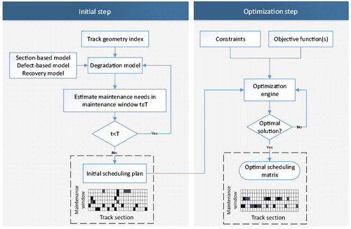
The optimization approach developed through this study, illustrated in Figure 4, includes two major steps, i.e. the initial step and the optimization step. In the initial step, the degradation and recovery models are used to estimate the maintenance needs in each maintenance window. This step is required to build the initial tamping schedule and is presented in detail in Sub-sections 4.1 and 4.2. In the next step, the tamping schedule is optimized with respect to the objective function, along with the constraints, which are presented in Section 4.3. Finally, a GA is used as an optimization engine to solve the problem.

Figure 4. The procedure for achieving an optimal tamping schedule.

4.1. Modelling the track geometry degradation and restoration

There exist a wide variety of models in the literature that have been used to model the track geometry degradation between two maintenance cycles and on the basis of recorded measurement data over time or in relation to usage. These models include the linear model (Caetano & Teixeira, 2015; Caetano & Teixeira, 2016; Khajehei et al., 2019; Lee et al., 2018), the exponential model (Peralta et al., 2018; Quiroga & Schnieder, 2012), the grey model (Chaolong, Weixiang, Futian, & Hanning, 2012; Xin, Famurewa, Gao, Kumar, & Zhang, 2016), and the Wiener process (Soleimanmeigouni, Ahmadi, Letot, Nissen, & Kumar, 2016), among other models. In the present study, the exponential model presented in equation (2)(2) $${\mathit{SDLL}}_{s,n}\left(t\right)={\mathit{SDLL}}_{s,n}^0.e^{b_s^0{(1+\omega )}^{(n-1)}\times (t-{T_{lt}}_s)}$$(2) has been used to model the track geometry degradation between two maintenance cycles. The exponential function is widely used to model track geometry degradation, due to the simplicity of the model and its ability to represent the underlying geometry degradation path (Soleimanmeigouni, Ahmadi, & Kumar, 2018): (2) $${\mathit{SDLL}}_{s,n}\left(t\right)={\mathit{SDLL}}_{s,n}^0.e^{b_s^0{(1+\omega )}^{(n-1)}\times (t-{T_{lt}}_s)}$$(2) where ${\mathit{SDLL}}_{s,n}\left(t\right)$ is the degradation value in the n^th tamping cycle for track section $sϵS$ at time t, $t\ge 0,$ ${\mathit{SDLL}}_{s,n}^0$ is the initial degradation value after the n^th tamping cycle for track section $sϵS,$ $b_s^0$ is the initial degradation rate for track section $sϵS,$ $\omega$ is the change in the degradation rate after tamping, n is the number of tamping cycles, n = [1,2,3,…,N], t denotes the time, and ${T_{lt}}_s$ is the time of the latest tamping intervention for track section $sϵS$ (it resets the local time of track section s after tamping to zero).

In order to model the evolution of the track geometry degradation in multiple maintenance cycles, it is necessary to model the tamping recovery. Performing tamping on the track geometry causes two changes in the degradation pattern. Firstly, tamping improves the geometry condition of the track, which will lead to a sudden change in the degradation level. However, tamping cannot restore the geometry condition to an ‘as-good-as-new’ state (Soleimanmeigouni, Ahmadi, Arasteh Khouy, & Letot, 2018). It must be noted that the effect of tamping decreases with an increase in the number of tamping interventions, resulting in a loss of tamping quality. Secondly, tamping causes a change in the degradation rate after tamping, which means that the rate of degradation will not remain constant in different maintenance cycles.

Therefore, in order to have an accurate prediction of the track geometry condition over multiple maintenance cycles, one must model the effect of tamping on the degradation pattern. Both the above-mentioned effects of tamping on the degradation pattern are considered in the prediction model used in this study. The change in the degradation rate $\omega$ is assumed to be a positive fixed value which shows that tamping will increase the degradation rate. In addition, the change in the degradation level is indicated by the recovery value $R,$ which is formulated as: (3) $$R_{s,n}=\frac{{\mathit{SDLL}}_{s,n}^0}{{\mathit{SDLL}}_{s,n}\left(t_{\mathit{tamp}}^{-}\right)}$$(3) where $R_{s,n}$ is the recovery value for track section $sϵS$ in the n^th tamping cycle and ${\mathit{SDLL}}_{s,n}\left(t_{\mathit{tamp}}^{-}\right)$ is the degradation value for track section $sϵS$ right before tamping. In order to estimate the tamping recovery, Equation (4)(4) $${\widehat{R}}_{s,n}=\{\begin{array}{c}\alpha +\beta {\mathit{SDLL}}_{s,n}\left(t_{\mathit{tamp}}^{-}\right), n=1\\ R_{s,1}.{(1-\phi )}^{n-1}, n>1\end{array}$$(4) is applied. In the first tamping cycle, n = 1, the recovery value is only dependent on the degradation value right before tamping. For the further tamping cycles, n > 1, the recovery value is dependent on the first recovery value and the quality loss factor ($\phi$): (4) $${\widehat{R}}_{s,n}=\{\begin{array}{c}\alpha +\beta {\mathit{SDLL}}_{s,n}\left(t_{\mathit{tamp}}^{-}\right), n=1\\ R_{s,1}.{(1-\phi )}^{n-1}, n>1\end{array}$$(4) where $R_{s,1}$ is the first achieved recovery value for track section $sϵS,$ $\phi$ is a fixed value bounded between 0 and 1 which shows the percentage of quality loss due to a tamping action, $\alpha$ is the regression coefficient, and $\beta$ is the coefficient for the degradation before the first tamping. 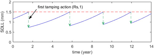By integrating Equations (2)(2) $${\mathit{SDLL}}_{s,n}\left(t\right)={\mathit{SDLL}}_{s,n}^0.e^{b_s^0{(1+\omega )}^{(n-1)}\times (t-{T_{lt}}_s)}$$(2) and (4)(4) $${\widehat{R}}_{s,n}=\{\begin{array}{c}\alpha +\beta {\mathit{SDLL}}_{s,n}\left(t_{\mathit{tamp}}^{-}\right), n=1\\ R_{s,1}.{(1-\phi )}^{n-1}, n>1\end{array}$$(4) , the evolution of the SDLL in multiple maintenance cycles can be simulated. Figure 5 shows the long-term evolution of the SDLL for one track section by considering a maintenance limit of 1.5 mm.

Figure 5. The evolution of the SDLL in multiple maintenance cycles.

4.2. Modelling the probability of UH2 defects

The UH2 defects of the longitudinal level, alignment and twist are considered in the optimization model used in the present study. In order to consider the UH2 defects in the optimization model, it is necessary to predict the probability of the occurrence of UH2 defects in track section $sϵS$ in maintenance window $t,$ i.e., $P_{s,t}.$ It has been shown that the probability of the occurrence of severe isolated defects is dependent on the typical track geometry indicators used to plan maintenance activities, e.g. the SDLL (Andrade & Teixeira, 2014; Soleimanmeigouni, Ahmadi, Khajehei & Nissen, 2020).

Based on the occurrence of UH2 defects, the track sections can be classified into two groups, namely sections without any UH2 defect and sections with at least one UH2 defect. Therefore, for the purpose of this study, the response variable $Y_{s,t}$ is defined as a binary variable which takes a value of one when there is at least one UH2 defect in the track section, and zero otherwise. When a response variable has only two possible values, the binary logistic regression model is widely used to model the relationship between the response variable and the explanatory variables.

Accordingly, binary logistic regression is used with the SDLL as the explanatory variable to estimate the probability of the occurrence of UH2 defects. By considering $Y_{s,t}$ as the response variable, the aim is to model the conditional probability $P\left(Y_{s,t}=1\left|{\mathit{SDLL}}_{s,n}\right(t)\right)=\pi ({\mathit{SDLL}}_{s,n}(t)).$ The probability of the occurrence of a UH2 defect $P\left(Y_{s,t}=1\left|{\mathit{SDLL}}_{s,n}\right(t)\right)$ can be obtained using: (5) $$P\left(Y_{s,t}=1\left|{\mathit{SDLL}}_{s,n}\right(t)\right)=\pi \left({\mathit{SDLL}}_{s,n}\right(t\left)\right)=\frac{e^{{\beta }_0+{\beta }_1{\mathit{SDLL}}_{s,n}\left(t\right)}}{1+e^{{\beta }_0+{\beta }_1{\mathit{SDLL}}_{s,n}\left(t\right)}}$$(5)

where ${\beta }_0\mathrm{ }\mathit{and}\mathrm{ }{\beta }_1$ are the model coefficients, which are estimated utilizing the maximum likelihood method.

4.3. Mathematical scheduling model

This sub-section presents the formulation of the OM-based tamping scheduling problem, described in Section 3, as a MILP model. To begin with, the objective function, equation (6)(6) $$\min E\left(C_{X,Z}\right)=\sum _{t\in T}\left(z_t.f+\sum _{s\in S}{x}_{s,t}.L_s.C_{pm}\right)+{\sum }_{t\in T}{\sum }_{s\in S}{P}_{s,t}.C_{\mathit{iso}}+{\sum }_{t\in T}{\sum }_{s\in S}{UL}_{s,t}.x_{s,t}.C_{UL}$$(6) , presents the detailed format of Equation (1)(1) $$C_{X,Z}=\mathit{minimize}\mathrm{ }{C}_{X,Z}^{\mathit{Tamping}}+C_{X,Z}^{UH2\mathrm{ }\mathit{defects}}+C_{X,Z}^{\mathit{Unused}\mathrm{ }\mathit{life}}$$(1) . The first part of the objective function considers the direct cost of performing tamping actions, which consists of two separate parts, namely a fixed cost and a variable cost. The fixed cost of tamping ($f>0$) represents the cost which needs to be paid if at least one track section requires tamping in a maintenance window.

However, this cost is independent of the number of tamped track sections in the maintenance window. On the other hand, the variable cost is associated with the performance of tamping on track sections and is dependent on the length of the track which is tamped. The second part of the objective function represents the cost associated with the occurrence of UH2 defects. The third part represents the cost associated with the unused life of track sections due to the earlier performance of tamping interventions: (6) $$\min E\left(C_{X,Z}\right)=\sum _{t\in T}\left(z_t.f+\sum _{s\in S}{x}_{s,t}.L_s.C_{pm}\right)+{\sum }_{t\in T}{\sum }_{s\in S}{P}_{s,t}.C_{\mathit{iso}}+{\sum }_{t\in T}{\sum }_{s\in S}{UL}_{s,t}.x_{s,t}.C_{UL}$$(6)

The unused life of track section $sϵS$ in the given maintenance window $tϵT$ is calculated using this formula: (7) $${UL}_{s,t}=\mathrm{ }\frac{1}{b_s}\mathrm{l}\mathrm{n}\left(\frac{\gamma }{{\mathit{SDLL}}_s}\right)$$(7) where ${UL}_{s,t}$ is the unused life of track section $sϵS$ in maintenance window $tϵT,$ $b_s$ and ${\mathit{SDLL}}_s\mathrm{ }$ are the degradation rate and SDLL value for track section $sϵS$ in maintenance window $tϵT,$ respectively, and $\gamma$ is the upper bound of the (corrective) maintenance limit.

The objective function must be minimized with respect to a set of constraints, which are elaborated in the sequence. Constraints (8) to (12) are related with the track geometry degradation and restoration. Constraint (8) represents the exponential degradation of the track sections. Constraints (9) and (10) express the recovery value for track section $sϵS.$ Constraint (11) reflects the number of tamping actions performed on track section $sϵS$ from the start until the current time (ct). Constraint (12) refers to the initial degradation value after tamping for track section $sϵS$ in the n^th tamping cycle: (8) $${\mathit{SDLL}}_{s,t}={\mathit{SDLL}}_{s,n}^0.e^{b_s^0{(1+\omega )}^{(n-1)}\times (t-{T_{lt}}_s)}\mathrm{ }\forall tϵT,\mathrm{ }sϵS$$(8) (9) $$R_{s,1}=\alpha +\beta {\mathit{SDLL}}_{s,1}\mathrm{ }\forall sϵS,\mathrm{ }n=1$$(9) (10) $$R_{s,n}=R_{s,1}.{(1-\phi )}^{n-1}\mathrm{ }\forall sϵS,\mathrm{ }n>1$$(10) (11) $$n=\sum _{t=1}^{ct}{x}_{s,t}\mathrm{ }\forall tϵT,\mathrm{ }sϵS$$(11) (12) $${\mathit{SDLL}}_{s,n}^0={\mathit{SDLL}}_{s,t}\times R_{s,n}\mathrm{ }\forall tϵT,\mathrm{ }sϵS$$(12)

In addition, constraints (13) and (14) enforce the maintenance limits on the geometry degradation of track sections, while Constraint (13) is the lower bound and constraint (14) is the upper bound for tamping activities: (13) $${\mathit{SDLL}}_{s,t}.x_{s,t}\ge \mathit{plan}\mathrm{ }\forall tϵT,\mathrm{ }sϵS$$(13) (14) $${\mathit{SDLL}}_{s,t}<\gamma \mathrm{ }\forall tϵT,\mathrm{ }sϵS$$(14)

Constraint (15) ensures that the total tamping time is less than the possession time assigned to maintenance window t. Equation (16)(16) $$T_t^M=T_t^{tp}+T_t^{cw}+T_t^{tr}\mathrm{\hspace{1em}}\forall tϵT$$(16) computes the total tamping time in maintenance window t. The total tamping time consists of three different times, namely the actual tamping time ($T_t^{tp}$), the travelling time ($T_t^{tr}$), and the warm-up and cool-down time ($T_t^{cw}$). Based on authors’ discussions with railway maintenance experts, it is highly important to consider the warm-up and cool-down time in the model, because ignoring this issue will, in most cases, create geometry defects in the track sections in question. Equation (17)(17) $$T_t^{tp}=\sum _{s=1}^S\frac{L_s}{V_{\mathit{tamp}}}.x_{s,t}\mathrm{\hspace{1em}}\forall tϵT,\mathrm{ }sϵS$$(17) gives the tamping time required for track section $sϵS$ based on the length of the track section $L_s$ and the tamping speed $V_{\mathit{tamp}}.$ Equation (18)(18) $$T_t^{tr}=\frac{\sum _{s=1}^S{L}_s(1-x_{s,t})}{V_{tr}}\mathrm{\hspace{1em}}\forall tϵT,\mathrm{ }sϵS$$(18) provides the total travelling time in each maintenance window based on the travelling speed $V_{tr}.$ Equation (19)(19) $$T_t^{cw}=\sum _{s=1}^S{y}_{t,s}.T_{cw}\mathrm{\hspace{1em}}\forall tϵT,\mathrm{ }sϵS$$(19) gives the total time required for warming up and cooling down in each tamping window. Constraint (20) ensures that the warming up and cooling down will not occur twice when performing tamping on two consecutive track sections. Constraint (21) ensures that in the case of tamping being performed on the last section, cooling down must be applied: (15) $$T_t^M\le T^P\mathrm{\hspace{1em}}\forall tϵT$$(15) (16) $$T_t^M=T_t^{tp}+T_t^{cw}+T_t^{tr}\mathrm{\hspace{1em}}\forall tϵT$$(16) (17) $$T_t^{tp}=\sum _{s=1}^S\frac{L_s}{V_{\mathit{tamp}}}.x_{s,t}\mathrm{\hspace{1em}}\forall tϵT,\mathrm{ }sϵS$$(17) (18) $$T_t^{tr}=\frac{\sum _{s=1}^S{L}_s(1-x_{s,t})}{V_{tr}}\mathrm{\hspace{1em}}\forall tϵT,\mathrm{ }sϵS$$(18) (19) $$T_t^{cw}=\sum _{s=1}^S{y}_{t,s}.T_{cw}\mathrm{\hspace{1em}}\forall tϵT,\mathrm{ }sϵS$$(19) (20) $$y_{s,t}\ge x_{s,t}-x_{s+1,t}\mathrm{ }\forall tϵT,\mathrm{ }s=1,2,\mathrm{ }\dots ,n-1$$(20) (21) $$y_{s,t}\ge x_{s,t}\mathrm{ }\forall \mathrm{ }tϵT,\mathrm{ }s=S$$(21)

Constraint (22) sets $z_t$ equal to 1 if there is at least one track section that is tamped in the t^th tamping window: (22) $$z_t\ge x_{s,t}\mathrm{\hspace{1em}}\forall tϵT,\mathrm{ }sϵS\mathrm{ }$$(22)

As per UIC (2008), it is recommended that tamping activities should start and finish on a straight line. If this is not possible, they can start or finish on circular curves. However, starting or finishing tamping operations on transition curves is forbidden, even if extreme care is taken. This is because it is difficult to achieve an acceptable run into and out of transition curves (UIC, 2008). Constraints (23) and (24) make sure that the track sections before and after sections on a transition curve will be tamped, if a track section in the curve needs tamping: (23) $$x_{t.s-1}\ge x_{t.s}.l_s\mathrm{\hspace{1em}}\forall tϵT,\mathrm{ }sϵS$$(23) (24) $$x_{t.s+1}\ge x_{t.s}.l_s\mathrm{\hspace{1em}}\forall tϵT,\mathrm{ }sϵS$$(24)

Another practical issue that is considered in the model is the performance of tamping on track sections located between two track sections that require tamping (structural dependence). Constraint (25) deals with this issue in the proposed model and schedules tamping on track section $sϵS,$ without considering its condition, if track sections s-1 and s + 1 need to be tamped. This constraint helps to keep the evenness of the track. Based on discussions with railway maintenance experts in the railway maintenance company Infranord, this constraint also depends on the tamping machine speed. Generally, if the tamping machine speed is high (as is the case with new tamping machines of high quality), then it is preferable to apply this constraint: (25) $$x_s\ge x_{s+1}+x_{s-1}-1\text{s}>1$$(25)

Lastly, constraints (26, 27) and (28) ensure that variables $x_{t,s},$ $y_{t,s},$ $l_s$ and $z_t$ are binary; (26) $$z_tϵ\left\{0,1\right\}\mathrm{ }\forall \mathrm{ }tϵT$$(26) (27) $$l_sϵ\left\{0,1\right\}\mathrm{ }\forall \mathrm{ }sϵS$$(27) (28) $$x_{t,s},\mathrm{ }{y}_{t,s}ϵ\left\{0,1\right\}\mathrm{ }\forall \mathrm{ }tϵT,\mathrm{ }sϵS$$(28)

5. Solution method

It has been proven that the tamping scheduling problem is a non-deterministic polynomial-time hard (NP-hard) problem; see, e.g., Peralta et al. (2018) and Zhang et al. (2013) for details. Consequently, standard optimization techniques, e.g., branch and bound, are not suitable for solving the tamping scheduling problem, especially for a large number of track sections (Zhang et al., 2013; Zhao, Chan, & Burrow, 2009). Therefore, a GA is used to find the optimal solution for the problem dealt with in this study. The GA has been proven to be suitable for solving NP-hard problems and has been applied by many researchers to solve various engineering problems in different fields, including tamping scheduling problems (Zhang et al., 2013; Zhao et al., 2009).

Initialization is one of the most important steps in the GA. Using heuristic initialization increases the efficiency of the GA, although an excessive use of heuristic initialization will decrease the exploration capacity of the algorithm (Osaba et al., 2014). Therefore, a heuristic method should be used for the initialization, which will result in initial logical solutions for the problem while ensuring the diversity of these solutions. Actually, the initial solutions are not generated randomly. Thus, the initial solutions created by the proposed heuristic method are always within a set of feasible solutions. The steps for creating the initial solutions are as follows:

1. Limit the number of tamped sections in each maintenance window to a maximum of 15% and a minimum of 5% of the total number of track sections.

2. Predict the degradation value of each track section using the degradation model (for the first upcoming maintenance window).

3. Generate a random number [0,1] to use for the current maintenance window:

   • If the random number is ‘1’, then a random number is generated between the minimum and maximum number of tamping interventions (based on step 1). The generated number indicates the number of sections selected for tamping.

   • Sort out the track sections in the worst condition.

   • Select n track sections (based on the generated random number) whose degradation values have exceeded the planning limit. If the number of sections with degradation values higher than the planning limit is greater than the number generated previously as described above, the worst-case sections will be selected as candidates and tamping of the others will be postponed to the next maintenance windows. If the number of sections with degradation values higher than the planning limit is smaller than the number generated previously as described above, then all the track sections above the planning limit are selected for tamping.

   • If the random number is ‘0’, the current maintenance window is not used.

4. Go back to step 2 and continue the process until the end of the planning horizon.

The proposed heuristic method, which is based on a two-step random selection, guarantees the diversity of the initial solutions while considering the condition of the track sections.

6. Case study

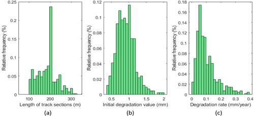
In order to test the proposed model, a case study was carried out using a data set collected from the Main Western Line in Sweden. The Main Western Line (Västra Stambanan) is the main railway line between Stockholm and Gothenburg. It is a double-track, electrified and remotely blocked line, used by both passenger and freight trains. The maximum speed of trains on the Main Western Line is around 200 km/h and the line consists of UIC 60 and SJ 50 rails, M1 ballast material, Pandrol e-clip fasteners and concrete sleepers. On this selected line, line section 414 between Sparreholm and Sköldinge stations was used for the case study. The length of the selected line section is about 18 km and it is divided into 97 track sections with different lengths, mostly from 100 m to 300 m. The length of each track section is fixed and provided by infrastructure managers. Figure 6a shows the distribution of the lengths of the track sections. As can be seen, the length of most of the track sections is around 200 m. The data on the line section used in the case study were collected for the time period between 2007 and 2018.

Figure 6. Histograms of the length of the track, the initial degradation value and the degradation rate.

For the purposes of the case study, the optimal tamping scheduling is determined by considering three different scenarios for the tamping limit ($\gamma$). The scenarios for the tamping limit ($\gamma )$ were defined by considering the relationship between the SDLL and the probability of the occurrence of UH2 defects and by applying three cut-off values, i.e. 0.1, 0.3 and 0.5. In the base case scenario, the cut-off value was 0.1, which meant that the $\gamma$ value was the corresponding SDLL for a probability of the occurrence of UH2 defects equal to 0.1. The second and third scenarios were defined by considering cut-off values equal to 0.3 and 0.5, respectively. Applying a smaller cut-off value (0.1 in the examined case) implies a pessimistic maintenance policy in which maintenance actions perform in a manner to minimize the occurrence of isolated defects. Therefore, it is expected to perform more maintenance actions in this policy, which will lead to a lower average of degradation values for track sections. On the other hand, a larger cut-off value (0.5 in this case study) implies an optimistic maintenance policy. In fact, in this policy there is a lower priority to recover geometry isolated defects. Thus, it is expected that track sections degrade more compare to the previous case and maintenance actions will be performed in the certain cases with higher risk of the occurrence of isolated defects.

The planning horizon was set to three years and maintenance windows were available every 6 months. The degradation model presented in Equation (2)(2) $${\mathit{SDLL}}_{s,n}\left(t\right)={\mathit{SDLL}}_{s,n}^0.e^{b_s^0{(1+\omega )}^{(n-1)}\times (t-{T_{lt}}_s)}$$(2) was used to predict the condition of each track section in the available maintenance windows. The initial degradation parameters were extracted from the dataset. Based on expert opinions, the change in the degradation rate after tamping was set to 5%. Figures 6b and c show the histograms of the degradation values and degradation rates, respectively. In order to estimate the probability of the occurrence of UH2 defects, Equation (5)(5) $$P\left(Y_{s,t}=1\left|{\mathit{SDLL}}_{s,n}\right(t)\right)=\pi \left({\mathit{SDLL}}_{s,n}\right(t\left)\right)=\frac{e^{{\beta }_0+{\beta }_1{\mathit{SDLL}}_{s,n}\left(t\right)}}{1+e^{{\beta }_0+{\beta }_1{\mathit{SDLL}}_{s,n}\left(t\right)}}$$(5) was used, considering the SDLL as the predictor. It should be notified that in this study the time to UH2 failures is not estimated. If the time to failure need to be analysed, it is important to take into account the censored data, as the exact time of failure is unknown. Readers are referred to Alemazkoor, Ruppert, and Meidani (2018) for more information.

In this study, the response variable$Y$ took a value of 0 whenever there was no UH2 defect in the track section, and a value of 1 whenever there was at least one UH2 defect in the track section. The data relating to the registered UH2 defects in the database for line section 414 were used to estimate the model parameters. The binary logistic regression for the proposed model is presented below: (29) $$P\left(Y|\mathit{SDLL}\right)=\frac{e^{8.09-3.78S\mathit{DLL}}}{1+e^{8.09-3.78S\mathit{DLL}}}$$(29)

The results of the model show a p-value less than the significant level (0.05) for the SDLL and show that this factor is statistically significant.

The parameters of the recovery model (part 1 of Equation (4)(4) $${\widehat{R}}_{s,n}=\{\begin{array}{c}\alpha +\beta {\mathit{SDLL}}_{s,n}\left(t_{\mathit{tamp}}^{-}\right), n=1\\ R_{s,1}.{(1-\phi )}^{n-1}, n>1\end{array}$$(4) ) were estimated by applying simple linear regression to the ratio between the SDLLs before and after the first tamping interventions for line section 414. The model for estimating the tamping recovery after the first tamping activity was formulated as follows: $$R_{s,1}=0.8-0.134.{\mathit{SDLL}}_{s,1}$$

For the second part of the recovery model, the percentage of the quality loss due to a tamping action ($\phi$) was set to 5% based on expert opinions.

The cost parameters and initial model parameters, presented in Tables 2 and 3, were set based on discussions with Trafikverket and Infranord maintenance experts. Regarding the cost associated with the occurrence of UH2 defects, it was assumed that the occurrence of UH2 defects would not lead to derailment and the cost was set based on Khajehei et al. (2019). In addition, the parameters of the GA were set according to Table 4.

Table 2. Cost parameters.

Description	Parameter	Cost (SEK)
Fixed cost of maintenance (per maintenance window)	$f$	150,000
Cost of preventive tamping (per metre)	$C_{pm}$	25
Cost of the probability of isolated defects	$C_{\mathit{iso}}$	11,000
Cost of unused life due to earlier performance of tamping action	$C_{UL}$	3,000

Table 3. Initial parameters to develop the model.

Description	Parameters	Value
Time horizon	T	3 years
Maintenance windows	t	6 months
Possession time for tamping work	$T^P$	6 hours
Warm-up and cool-down time	$T_{cw}$	20 mins.
Speed of tamping machine during tamping	$V_{\mathit{tamp}}$	1 km/h
Speed of tamping machine during travelling	$V_{tr}$	80 km/h
Lower bound of preventive limit	plan	1.2 mm

Table 4. Parameters of the genetic algorithm.

Parameter	Value
Size of the population	150
Number of generations	300
Cross-over percentage	0.9
Mutation percentage	0.5
Mutation probability	0.005

6.1. Results of tamping scheduling

By solving the scheduling problem using the GA, the results relating to the optimal tamping schedules for different scenarios were obtained. These results are presented in detail in Table 5, including the number of tamping actions (# tamping), the total length of track tamped and the maintenance costs for all the three scenarios. As can be seen, for the base case scenario, a higher number of track sections were scheduled for tamping because a more conservative approach was adopted to reduce the number of occurrences of UH2 defects. The other two scenarios, on the other hand, are more optimistic about the occurrence of UH2 defects; i.e. the SDLL had to exceed a larger value compared to the base case scenario before a PM action was performed to prevent the occurrence of UH2 defects.

Table 5. Detailed results for the optimal tamping schedule.

Maintenance window	(1(1) $$C_{X,Z}=\mathit{minimize}\mathrm{ }{C}_{X,Z}^{\mathit{Tamping}}+C_{X,Z}^{UH2\mathrm{ }\mathit{defects}}+C_{X,Z}^{\mathit{Unused}\mathrm{ }\mathit{life}}$$(1) )	(2(2) $${\mathit{SDLL}}_{s,n}\left(t\right)={\mathit{SDLL}}_{s,n}^0.e^{b_s^0{(1+\omega )}^{(n-1)}\times (t-{T_{lt}}_s)}$$(2) )	(3(3) $$R_{s,n}=\frac{{\mathit{SDLL}}_{s,n}^0}{{\mathit{SDLL}}_{s,n}\left(t_{\mathit{tamp}}^{-}\right)}$$(3) )	(4(4) $${\widehat{R}}_{s,n}=\{\begin{array}{c}\alpha +\beta {\mathit{SDLL}}_{s,n}\left(t_{\mathit{tamp}}^{-}\right), n=1\\ R_{s,1}.{(1-\phi )}^{n-1}, n>1\end{array}$$(4) )	(5(5) $$P\left(Y_{s,t}=1\left|{\mathit{SDLL}}_{s,n}\right(t)\right)=\pi \left({\mathit{SDLL}}_{s,n}\right(t\left)\right)=\frac{e^{{\beta }_0+{\beta }_1{\mathit{SDLL}}_{s,n}\left(t\right)}}{1+e^{{\beta }_0+{\beta }_1{\mathit{SDLL}}_{s,n}\left(t\right)}}$$(5) )	(6)	Total
First scenario (base case)
# tamping	14	0	10	0	18	0	42
Total length tamped (metres)	2354	0	1657	0	3357	0	7368
Fixed cost							4.500˟10^5
Preventive tamping cost							1.473˟10^5
Corrective tamping cost							1.671˟10^5
Unused life cost							2.601˟10^5
Total cost (SEK)							10.246˟10^5
Second scenario
# tamping	9	0	7	0	0	0	16
Total length tamped (metres)	1432	0	1265	0	0	0	2697
Fixed cost							3.000˟10^5
Preventive tamping cost							0.539˟10^5
Corrective tamping cost							2.210˟10^5
Unused life cost							1.188˟10^5
Total cost (SEK)							6.251˟10^5
Third scenario
# tamping	9	0	0	4	0	0	13
Total length tamped (metres)	1457	0	0	711	0	0	2168
Fixed cost							3.000˟10^5
Preventive tamping cost							0.434˟10^5
Corrective tamping cost							2.540˟10^5
Unused life cost							1.254˟10^5
Total cost (SEK)							7.228˟10^5

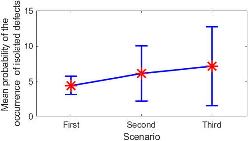
Regarding the optimal scenario, the second scenario provides the minimum maintenance cost, although the third scenario results in the smallest number of tamping actions and the shortest total length of tamped track. The reason is the existence of the cost component related to the probability of the occurrence of UH2 defects, which increase exponentially. Moreover, Figure 7 depicts the mean probability of the occurrence of UH2 defects for all the three scenarios. The figure clearly shows that the mean probability of the occurrence of UH2 defects for the second and third scenarios is higher than that for the base case scenario.

Figure 7. Mean probability of occurrence of isolated defects for the whole line for different For Peer Review Only scenarios.

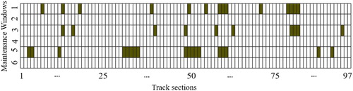
Figure 8 displays the optimal tamping schedule obtained by the GA for the base case scenario. The figure shows that three maintenance windows were used in the optimal schedule plan as a result of grouping the tamping activities. In addition, because the unused life is considered in the proposed model, the model tries to schedule tamping as late as possible to minimize the unused life of track sections. Therefore, the proposed model enables IMs to assess the scheduling plan with respect to the expected risk of the occurrence of UH2 defects.

Figure 8. The optimal tamping schedule for the base case scenario.

6.2. Effect of a change in the degradation rate parameter on the final scheduling result

As mentioned in Sub-section 4.1, performing tamping on a track section causes two changes in the degradation pattern, i.e., a change in the degradation rate and a loss of track quality due to the destructive effect of tamping. This sub-section treats the effect of considering a change in the degradation rate parameter ($\omega$) (see Equation (2)(2) $${\mathit{SDLL}}_{s,n}\left(t\right)={\mathit{SDLL}}_{s,n}^0.e^{b_s^0{(1+\omega )}^{(n-1)}\times (t-{T_{lt}}_s)}$$(2) ) on the final scheduling results. The results of optimal scheduling for the base case scenario for the model with and the model without $\omega$ are compared. These results are presented in Table 6, including the total number of tamping actions (# tamping), the total length of track tamped and the total maintenance costs. As can be seen, the model without $\omega$ underestimates the total number of tamping actions, as well as underestimating the total maintenance costs by 2%.

Table 6. The results of optimal scheduling for the base case scenario, with and without considering the change in the degradation rate parameter.

Change in degradation rate after tamping	# tamping	Length of tamped track sections (metres)	Total cost
$\omega =0$	40	7026	$10.010\mathrm{˟}{10}^5$
$\omega =5\mathrm{\%}$	42	7368	$10.246\mathrm{˟}{10}^5$

6.3. Effect of a fixed cost of tamping

The fixed cost of tamping is generally dependent on the number of maintenance machines used, the amount of fuel consumed, the logistics, and the crew’s salary and accommodation, among other causes of relevant expenditure. Therefore, the fixed cost of tamping directly depends on the company’s resources and can vary from one contractor to other. In this study, a sensitivity analysis was performed to evaluate the effect of different fixed costs of tamping on the optimal tamping scheduling.

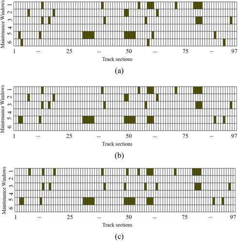
When performing this analysis, all the initial parameters presented in Tables 3 and 4 were taken to be the same as previously, except for the fixed cost of tamping. The effect on the base case scenario of three different fixed tamping costs, i.e., 10,000, 50,000 and 150,000 SEK, was investigated, and the results are shown in Figure 9. As can be seen, the lower the fixed cost of tamping is, the more maintenance windows are occupied for tamping operations. When there is a lower fixed cost, the model tends to schedule tamping actions when the track sections approach the upper bound of the maintenance limit, as the obtained benefit for releasing a maintenance window is rather small in relation to the total maintenance cost.

Figure 9. Optimal tamping schedules for the base case scenario for a fixed cost of maintenance equal to a) 10,000 SEK, b) 50,000 SEK and c) 150,000 SEK.

6.4. Effect of the unused life of track sections on the optimal tamping scheduling

Sometimes it is more economical for maintenance contractors to perform tamping earlier, i.e. to perform tamping actions on a track section before the upper maintenance limit has been reached. This may happen for different reasons, e.g. to reduce the probability of the occurrence of UH2 defects and to exploit the availability of tamping resources. However, as reported by Andrews (2013), while tamping actions will improve the condition of the ballast, the squeezing and vibrating of the ballast by tamping tines will break up the ballast particles. Considering this destructive effect of tamping on the ballast particles, increasing the frequency of tamping actions may shorten the life cycle of the track.

In the proposed model, to avoid the unnecessary performance of earlier tamping actions, the unused life is included in the model. In the case study, the effect of the unused life on the optimal tamping scheduling for the base case scenario was investigated. To achieve this, the optimal base case schedule with the unused life included in the model was compared with the optimal base case schedule without the unused life included in the model. Table 7 presents the results of this comparison. As can be seen, the model which does not include the unused life in the objective function selects more track sections as candidates for conducting earlier tamping actions. Therefore, in the long term, models which do not include the unused life will shorten the life cycle of the track sections.

Table 7. The results of the model with and without the unused life included in the objective function.

Maintenance window	(1(1) $$C_{X,Z}=\mathit{minimize}\mathrm{ }{C}_{X,Z}^{\mathit{Tamping}}+C_{X,Z}^{UH2\mathrm{ }\mathit{defects}}+C_{X,Z}^{\mathit{Unused}\mathrm{ }\mathit{life}}$$(1) )	(2(2) $${\mathit{SDLL}}_{s,n}\left(t\right)={\mathit{SDLL}}_{s,n}^0.e^{b_s^0{(1+\omega )}^{(n-1)}\times (t-{T_{lt}}_s)}$$(2) )	(3(3) $$R_{s,n}=\frac{{\mathit{SDLL}}_{s,n}^0}{{\mathit{SDLL}}_{s,n}\left(t_{\mathit{tamp}}^{-}\right)}$$(3) )	(4(4) $${\widehat{R}}_{s,n}=\{\begin{array}{c}\alpha +\beta {\mathit{SDLL}}_{s,n}\left(t_{\mathit{tamp}}^{-}\right), n=1\\ R_{s,1}.{(1-\phi )}^{n-1}, n>1\end{array}$$(4) )	(5(5) $$P\left(Y_{s,t}=1\left|{\mathit{SDLL}}_{s,n}\right(t)\right)=\pi \left({\mathit{SDLL}}_{s,n}\right(t\left)\right)=\frac{e^{{\beta }_0+{\beta }_1{\mathit{SDLL}}_{s,n}\left(t\right)}}{1+e^{{\beta }_0+{\beta }_1{\mathit{SDLL}}_{s,n}\left(t\right)}}$$(5) )	(6(6) $$\min E\left(C_{X,Z}\right)=\sum _{t\in T}\left(z_t.f+\sum _{s\in S}{x}_{s,t}.L_s.C_{pm}\right)+{\sum }_{t\in T}{\sum }_{s\in S}{P}_{s,t}.C_{\mathit{iso}}+{\sum }_{t\in T}{\sum }_{s\in S}{UL}_{s,t}.x_{s,t}.C_{UL}$$(6) )	Total
Model without unused life
# tamping	17	14	0	0	13	0	43
Total length tamped (metres)	2796	2578	0	0	2274	0	7468
Consumed possession time	6.0	5.4	0	0	4.4	0	15.8
Model with unused life (base case)
# tamping	14	0	10	0	18	0	42
Total length tamped (metres)	2354	0	1657	0	3357	0	7368
Consumed possession time	5.6	0	4.5	0	5.8	0	15.9

6.5. Effect of the tamping machine speed on the optimal tamping scheduling

Tamping machines can be classified into different categories on the basis of their speed, which is mainly influenced by the number of sleepers that can be tamped simultaneously (Soleimanmeigouni, 2019). On main lines with a high traffic density and high speed and on heavy haul lines, it is generally the case that many trains pass along the track per day. On these lines, the maintenance windows are short (Zaayman, 2017). Therefore, using tamping machines with a high production rate is essential to maintain a high train punctuality by performing tamping operations within the short possession times. In the case study, the impact of the tamping machine speed during tamping and travelling on the optimal tamping schedule for the base case scenario is explored. For this purpose, the optimization procedure was performed for three tamping machines with different tamping speeds, i.e., 0.5 km/h, 1 km/h and 1.5 km/h. Regarding the travelling speed, the working performance (consumed possession time for tamping work) are compared for three different machines with travelling speeds of 80 km/h, 100 km/h and 120 km/h.

Figure 10 presents the results of the sensitivity analysis performed on the total working performance (possession time consumption). As can be seen, the tamping speed of the tamping machine highly affects the total working performance, while the travelling speed has a negligible effect on it. The results show that a tamping machine with a low performance (0.5 km/h) will increase the total possession time by about 34% compared to the base case (1.0 km/h). In addition, a tamping machine with a high tamping speed (1.5 km/h), will reduce the total possession time by about 15%.

Figure 10. Effect of the tamping speed and travelling speed of the tamping machine on the total working performance.

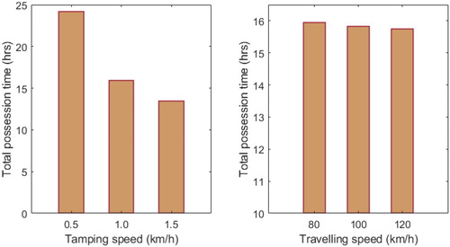
Regarding the travelling speed, the maximum improvement with regard to the total consumed possession time will be about 1.2%, which will have almost no effect on the final result. Furthermore, Table 8 presents the effect of the tamping machine speed on the total maintenance cost. As can be seen in this table, using a tamping machine with a low production rate (0.5 km/hr) will highly increase the total maintenance costs, while using a tamping machine with a high production rate (1.5 km/hr) will have no effect on the total maintenance costs. The results can be interpreted as indicating that, since there is a limited possession time in each maintenance window, using a tamping machine with a low performance requires the utilization of more maintenance windows to maintain the quality of the track. In addition, the total maintenance costs for a tamping machine with a high production rate are the same as those for the base case, because the benefits (bonus) of finishing the tasks in a shorter time than the assigned possession time have not been considered.

Table 8. Effect of the tamping speed of the tamping machine on the total maintenance costs.

Tamping speed (km/h)	Total maintenance costs (SEK)
0.5	13.101˟10^5
1.0 (base case)	10.246˟10^5
1.5	10.246˟10^5

Based on these results, it can be concluded that tamping machines with higher tamping speeds provide greater flexibility and more opportunities for maintenance contractors to perform tamping on more track sections (if necessary) in a shorter period of time. In addition, the travelling speed of the tamping machine will not highly affect the optimal tamping schedule or the maintenance costs. Finally, it is worth mentioning that besides the speed of the tamping machine, the experience of the driver of the tamping machine is highly important. In this study, it is assumed that the driver of the tamping machine possessed enough experience not to affect the tamping machine speed negatively.

7. Conclusions

The aim of this study has been to provide an OM optimization model for the problem of tamping scheduling. For this purpose, the objective function is set in such a way as to minimize the total maintenance costs and the number of unplanned tamping actions due to the occurrence of isolated defects. The standard deviation of the longitudinal level (SDLL) and the extreme values of isolated defects of the longitudinal level, alignment, and twist are used to represent the track geometry condition. An exponential model and binary logistic regression functions have been used to model the track geometry degradation and to predict the occurrence of isolated defects, respectively.

The tamping scheduling problem is formulated as a mixed integer linear programming (MILP) model. In the developed model, OM has been considered in the optimization model in the form of economic and structural dependence. In practice, it is well-known that there is a limited time for tamping activities and there exist different types of tamping machines with different levels of efficiency. The proposed model considers this issue and provides an optimal tamping schedule within the assigned possession time. The developed objective function in the programming model considers three main components, i.e., the direct cost of preventive tamping, the cost of the probability of the occurrence of isolated defects, and the unused life of a track section due to the earlier performance of tamping actions. A genetic algorithm has been used to determine the optimal solution to the problem.

The proposed model has been tested on real-life data collected from the Main Western Line in Sweden. The proposed model enables infrastructure managers to examine the effect of different scenarios for the control and management of isolated defects of the track geometry. In fact, in the proposed model it is possible to apply different scenarios based on the characteristics of the track line for planning maintenance activities to rectify isolated defects. In the case of a high-priority track line for passenger trains, it is desirable to have the minimum number of isolated defects as such defects highly affect the passenger comfort and cause traffic delays.

Therefore, the maintenance of such a line requires the definition of a proper scenario for the management of isolated defects by allocating a proper threshold for triggering maintenance actions. This is achieved in the proposed model by linking the probability of the occurrence of isolated defects with the level of the standard deviation of the longitudinal level. It has been shown that prediction of the track geometry condition without considering the destructive effect of tamping (a change in the degradation rate and a quality loss after tamping) will lead to underestimation of the maintenance needs. It has been found that it is important to consider the effect of the unused life of track sections to reduce the earlier performance of tamping actions. It is important to point out that the earlier performance of tamping actions will reduce the useful life of the track due to the destructive effect of tamping. The results show that the speed of the tamping machine can highly affect not only the optimal tamping schedule, but also the total maintenance cost. However, the travelling speed of the tamping machine has a minor effect on the final results and can be ignored. Therefore, it is highly recommended that, when determining the optimal tamping schedule, the speed of the tamping machine should be considered in the model.

One possible future research task would be to investigate the effect of considering the location of the tamping machine in the model. In addition, it must be noted that, in practice, tamping operations can be stopped because of problems associated with malfunctioning of the tamping machine. Hence, further research could also focus on the reliability of tamping machines as part of the scheduling problem.

Notations list
S	=	set of railway track sections, with the number of 1 to S
T	=	the given planning horizon
$\mathit{SDLL}$	=	the standard deviation of the longitudinal level
${\mathit{SDLL}}_{s,n}^0$	=	the initial degradation value after the nth tamping cycle for track section $sϵS$
$b_s^0$	=	the initial degradation rate for track section $sϵS$
$\omega$	=	a constant value which shows the change in the degradation rate after tamping
$\phi$	=	a constant value which shows the percentage of quality loss due to a tamping action
${T_{lt}}_s$	=	the time of the latest tamping intervention for track section $sϵS$
$C_{UL}$	=	the cost of the unused life due to the earlier performance of tamping actions (SEK/year)
$\mathit{f}$	=	the fixed cost of maintenance based on the available machines and crew
$C_{pm}$	=	the cost of a preventive tamping operation (per metre)
$C_{\mathit{iso}}$	=	the cost of the probability of the occurrence of isolated defects
$L_s$	=	the length of track section $sϵS$
$n$	=	the number of tamping actions
PM	=	preventive maintenance
CM	=	corrective maintenance
$R_{s,1}$	=	the first recovery value for track section $sϵS,$ which is dependent on the degradation value before tamping
$R_{s,n}$	=	the recovery value for track section $sϵS$ in the nth maintenance cycle (n > 1)
$T^P$	=	the possession time for tamping work (in hours)
$T_t^M$	=	the total tamping time in maintenance window $tϵT$
$T_t^{tp}$	=	the time required to perform tamping on a track section
$T_t^{tr}$	=	the time required to travel between track sections
$T_t^{cw}$	=	the time required to warm up and cool down the tamping machine
$V_{\mathit{tamp}}$	=	the tamping machine speed (km/h)
$V_{tr}$	=	the tamping machine travelling speed (km/h)
${UL}_{s,t}$	=	the unused life loss of track section $sϵS$ in maintenance window $tϵT$
$x_{s,t}$	=	binary variable which is 1 if track section $sϵS$ in maintenance window $tϵT$ needs to be tamped and 0 otherwise
$y_{t,s}$	=	binary variable for warming up and cooling down which is 1 if track section $sϵS$ needs to be tamped in maintenance window t and 0 otherwise
$z_t$	=	binary variable which is 1 if any track section needs to be tamped in maintenance window t and 0 otherwise
$l_s$	=	binary variable which is 1 if track section $sϵS$ is on a curve and 0 otherwise
$P_{s,t}$	=	the probability of occurrence of isolated defects for track section $sϵS$ in the tth time period

Acknowledgements

The authors would like to thank Trafikverket (the Swedish Transport Administration), Luleå Railway Research Center (JVTC) and Bana Väg För Framtiden (BVFF) for their technical and financial support provided during this project. Specific thanks are extended to the SIMTRACK project partners for their continuous technical and professional support and for sharing their expertise. The authors also wish to thank Roland Bång and Mikael Åstrand from Infranord for his valuable inputs and for sharing his experience with us. Finally, the authors would like to thank the anonymous reviewers for their productive comments, which have helped in improving the quality of the paper.

Disclosure statement

No potential conflict of interest was reported by the authors.

Notes

1 The possession time is defined as the time assigned for tamping activities, during which the track is free of traffic and regular service.

References

- Alemazkoor, N., Ruppert, C. J., & Meidani, H. (2018). Survival analysis at multiple scales for the modeling of track geometry deterioration. Proceedings of the Institution of Mechanical Engineers, Part F: Journal of Rail and Rapid Transit, 232(3), 842–850. doi:https://doi.org/10.1177/0954409717695650
- Andrade, A. R., & Teixeira, P. F. (2011). Uncertainty in rail-track geometry degradation: Lisbon-Oporto line case study. Journal of Transportation Engineering, 137(3), 193–200. doi:https://doi.org/10.1061/. (ASCE)TE.1943-5436.0000206. doi:https://doi.org/10.1061/(ASCE)TE.1943-5436.0000206
- Andrade, A. R., & Teixeira, P. F. (2014). Unplanned-maintenance needs related to rail track geometry. Proceedings of the Institution of Civil Engineers - Transport, 167(6), 400–410. doi:https://doi.org/10.1680/tran.11.00060
- Andrews, J. (2013). A modelling approach to railway track asset management. Proceedings of the Institution of Mechanical Engineers, Part F: Journal of Rail and Rapid Transit, 227(1), 56–73. doi:https://doi.org/10.1177/0954409712452235
- Budai, G., Huisman, D., & Dekker, R. (2006). Scheduling preventive railway maintenance activities. Journal of the Operational Research Society, 57(9), 1035–1044. doi:https://doi.org/10.1057/palgrave.jors.2602085
- Budai-Balke, G., Dekker, R., & Kaymak, U. (2009). Genetic and memetic algorithms for scheduling railway maintenance activities (Report EI 2009-30). Rotterdam: Erasmus University Rotterdam, Econometric Institute.
- Caetano, L. F., & Teixeira, P. F. (2015). Optimisation model to schedule railway track renewal operations: A life-cycle cost approach. Structure and Infrastructure Engineering, 11(11), 1524–1536. doi:https://doi.org/10.1080/15732479.2014.982133
- Caetano, L. F., & Teixeira, P. F. (2016). Predictive maintenance model for ballast tamping. Journal of Transportation Engineering, 142(4), 04016006. doi:https://doi.org/10.1061/(ASCE)TE.1943-5436.0000825
- Castanier, B., Grall, A., & Bérenguer, C. (2005). A condition-based maintenance policy with non-periodic inspections for a two-unit series system. Reliability Engineering & System Safety, 87(1), 109–120. doi:https://doi.org/10.1016/j.ress.2004.04.013
- Chaolong, J., Weixiang, X., Futian, W., & Hanning, W. (2012). Track irregularity time series analysis and trend forecasting. Discrete Dynamics in Nature and Society, 2012, 1–15. doi:https://doi.org/10.1155/2012/387857
- Dao, C., Basten, R., & Hartmann, A. (2018). Maintenance scheduling for railway tracks under limited possession time. Journal of Transportation Engineering, Part A: Systems, 144(8), 04018039. doi:https://doi.org/10.1061/JTEPBS.0000163
- EN 13848-5. (2008). Railway applications – track – track geometry quality. Part 5: Geometric quality levels. Brussels: European Committee for Standardization (CEN).
- Gustavsson, E. (2015). Scheduling tamping operations on railway tracks using mixed integer linear programming. EURO Journal on Transportation and Logistics, 4(1), 97–112. doi:https://doi.org/10.1007/s13676-014-0067-z
- He, Q., Li, H., Bhattacharjya, D., Parikh, D. P., & Hampapur, A. (2015). Track geometry defect rectification based on track deterioration modelling and derailment risk assessment. Journal of the Operational Research Society, 66(3), 392–404. doi:https://doi.org/10.1057/jors.2014.7
- Khajehei, H., Ahmadi, A., Soleimanmeigouni, I., & Nissen, A. (2019). Allocation of effective maintenance limit for railway track geometry. Structure and Infrastructure Engineering, 15(12), 1597–1612. doi:https://doi.org/10.1080/15732479.2019.1629464
- Lee, J. S., Choi, I. Y., Kim, I. K., & Hwang, S. H. (2018). Tamping and renewal optimization of ballasted track using track measurement data and genetic algorithm. Journal of Transportation Engineering, Part A: Systems, 144(3), 04017081. doi:https://doi.org/10.1061/JTEPBS.0000120
- Macedo, R., Benmansour, R., Artiba, A., Mladenović, N., & Urošević, D. (2017). Scheduling preventive railway maintenance activities with resource constraints. Electronic Notes in Discrete Mathematics, 58, 215–222. doi:https://doi.org/10.1016/j.endm.2017.03.028
- Nicolai, R. P., & Dekker, R. (2008). Optimal maintenance of multi-component systems: A review. In Khairy A.H. Kobbacy and D.N. Prabhakar Murthy (Eds.), Complex system maintenance handbook (pp. 263–286). London: Springer.
- Osaba, E., Carballedo, R., Diaz, F., Onieva, E., Lopez, P., & Perallos, A. (2014). On the influence of using initialization functions on genetic algorithms solving combinatorial optimization problems: A first study on the TSP. In IEEE Conference on Evolving and Adaptive Intelligent Systems (EAIS). doi:https://doi.org/10.1109/EAIS.2014.6867465
- Pargar, F., Kauppila, O., & Kujala, J. (2017). Integrated scheduling of preventive maintenance and renewal projects for multi-unit systems with grouping and balancing. Computers & Industrial Engineering, 110, 43–58. doi:https://doi.org/10.1016/j.cie.2017.05.024
- Peralta, D., Bergmeir, C., Krone, M., Galende, M., Menéndez, M., Sainz-Palmero, G. I., … Benitez, J.M. (2018). Multiobjective optimization for railway maintenance plans. Journal of Computing in Civil Engineering, 32(3), 04018014. doi:https://doi.org/10.1061/(ASCE)CP.1943-5487.0000757
- Pham, H. (2003). Recent studies in software reliability engineering. In Hoang Pham (Ed.), Handbook of reliability engineering (pp. 285–302). London: Springer.
- Quiroga, L. M., & Schnieder, E. (2012). Monte Carlo simulation of railway track geometry deterioration and restoration. Proceedings of the Institution of Mechanical Engineers, Part O: Journal of Risk and Reliability, 226(3), 274–282. doi:https://doi.org/10.1177/1748006X11418422
- Sharma, S., Cui, Y., He, Q., Mohammadi, R., & Li, Z. (2018). Data-driven optimization of railway maintenance for track geometry. Transportation Research Part C: Emerging Technologies, 90, 34–58. doi:https://doi.org/10.1016/j.trc.2018.02.019
- Soleimanmeigouni, I. (2019). Predictive models for railway track geometry degradation (Doctoral thesis). Luleå University of Technology.
- Soleimanmeigouni, I., Ahmadi, A., & Kumar, U. (2018). Track geometry degradation and maintenance modelling: A review. Proceedings of the Institution of Mechanical Engineers, Part F: Journal of Rail and Rapid Transit, 232(1), 73–102. doi:https://doi.org/10.1177/0954409716657849
- Soleimanmeigouni, I., Ahmadi, A., Arasteh Khouy, I., & Letot, C. (2018). Evaluation of the effect of tamping on the track geometry condition: A case study. Proceedings of the Institution of Mechanical Engineers, Part F: Journal of Rail and Rapid Transit, 232(2), 408–420. doi:https://doi.org/10.1177/0954409716671548
- Soleimanmeigouni, I., Ahmadi, A., Khajehei, H., & Nissen, A. (2020). Investigation of the effect of the inspection intervals on the track geometry condition. Structure and Infrastructure Engineering, 16(8), 1138–1139. doi:https://doi.org/10.1080/15732479.2019.1687528
- Soleimanmeigouni, I., Ahmadi, A., Letot, C., Nissen, A., & Kumar, U. (2016). Cost-based optimization of track geometry inspection. In 11th World Congress of Railway Research, Milan, Italy.
- Soleimanmeigouni, I., Ahmadi, A., Nissen, A., & Xiao, X. (2020). Prediction of railway track geometry defects: A case study. Structure and Infrastructure Engineering, 16(7), 987–1001. doi:https://doi.org/10.1080/15732479.2019.1679193
- Soleimanmeigouni, I., Xiao, X., Ahmadi, A., Xie, M., Nissen, A., & Kumar, U. (2018). Modelling the evolution of ballasted railway track geometry by a two-level piecewise model. Structure and Infrastructure Engineering, 14(1), 33–45. doi:https://doi.org/10.1080/15732479.2017.1326946
- Thomas, L. (1986). A survey of maintenance and replacement models for maintainability and reliability of multi-item systems. Reliability Engineering, 16(4), 297–309. doi:https://doi.org/10.1016/0143-8174(86)90099-5
- Trafikverket. (2015). Banöverbyggnad – spårläge – krav vid byggande och underhåll (Track superstructure – track geometry – requirements for renewal and maintenance [in Swedish]). Report No. TDOK 2013:0347 v3.0. Borlänge, Sweden: Trafikverket.
- UIC. (2008). Best practice guide for optimum track geometry durability. Paris: France: ETF – Railway Technical Publications.
- Vale, C., Ribeiro, I. M., & Calçada, R. (2012). Integer programming to optimize tamping in railway tracks as preventive maintenance. Journal of Transportation Engineering, 138(1), 123–131. doi:https://doi.org/10.1061/(ASCE)TE.1943-5436.0000296
- Wang, H. (2002). A survey of maintenance policies of deteriorating systems. European Journal of Operational Research, 139(3), 469–489. doi:https://doi.org/10.1016/S0377-2217(01)00197-7
- Wen, M., Li, R., & Salling, K. B. (2016). Optimization of preventive condition-based tamping for railway tracks. European Journal of Operational Research, 252(2), 455–465. doi:https://doi.org/10.1016/j.ejor.2016.01.024
- Xin, T., Famurewa, S. M., Gao, L., Kumar, U., & Zhang, Q. (2016). Grey-system-theory-based model for the prediction of track geometry quality. Proceedings of the Institution of Mechanical Engineers, Part F: Journal of Rail and Rapid Transit, 230(7), 1735–1744. doi:https://doi.org/10.1177/0954409715610603
- Zaayman, L. (2017). The basic principles of mechanized track maintenance (3rd ed.). Leverkusen: PMC Media House.
- Zhang, T., Andrews, J., & Wang, R. (2013). Optimal scheduling of track maintenance on a railway network. Quality and Reliability Engineering International, 29(2), 285–297. doi:https://doi.org/10.1002/qre.1381
- Zhao, J., Chan, A., & Burrow, M. (2009). A genetic-algorithm-based approach for scheduling the renewal of railway track components. Proceedings of the Institution of Mechanical Engineers, Part F: Journal of Rail and Rapid Transit, 223(6), 533–541. doi:https://doi.org/10.1243/09544097JRRT273