
 ?Mathematical formulae have been encoded as MathML and are displayed in this HTML version using MathJax in order to improve their display. Uncheck the box to turn MathJax off. This feature requires Javascript. Click on a formula to zoom.
Abstract
Optimization of the duration of Structural Health Monitoring (SHM) campaigns is rarely performed. This article provides a utility-based solution to posteriorly determine: i) optimal monitoring durations and ii) the extension of the service life of the welds on a steel bridge deck. The approach is illustrated with a case study focusing on remaining fatigue life estimation of the welds on the orthotropic steel deck of the Great Belt Bridge, in Denmark. The identification of the optimal monitoring duration and the decision about extending the service life of the welds are modelled by maximizing the expected benefits and minimizing the structural risks. The results are a parametric analysis, mainly on the effect of the target probability, benefit, cost of failure, cost of rehabilitation, cost of monitoring and discount rate on the posterior utilities of monitoring strategies and the choice of service life considering the risk variability and the costs and benefits models. The results show that the decision on short-term monitoring, i.e., 1 week every six months, is overall the most valued SHM strategy. In addition, it is found that the target probability is the most sensitive parameter affecting the optimal SHM durations and service life extension of the welds.
1. Introduction
Many studies on Structural Health Monitoring (SHM) have been made available in recent decades (e.g., Balageas, Fritzen, & Güemes, Citation2010; Farrar & Worden, 2007; Sohn et al., Citation2003). These studies focus mainly on data acquisition, normalization, cleaning, feature extraction and information condensation (Farrar et al., 2003; Farrar & Worden, Citation2012; Sohn et al., Citation2003). In the past decade, one of the main research topics in SHM was using monitoring for the management of structures (Okasha & Frangopol, Citation2012; Orcesi & Frangopol, Citation2011; Pozzi, Zonta, Wang, & Chen, Citation2010). Among these works, Vanik et al. presented a Bayesian probabilistic approach to SHM (Vanik, Beck, & Au, Citation2000). Wenzel et al. related the life cycle management for civil structures to SHM (Wenzel, Veit-Egerer, Widmann, & To, Citation2011). Flynn and Todd (Citation2010) developed an approach for optimising sensor placement of a SHM system.
Herein, the optimal SHM system is the one leading to the lowest Bayes risk (expected loss) in the context of the operational modelling of the SHM (Flynn & Todd, Citation2010; Todd, Haynes, & Flynn, Citation2011). In continuation of research progress, it has been gradually acknowledged that without a decision analytical framework including the structural system performance, the SHM information cannot be optimally utilized for the structural integrity management. Pozzi & Der Kiureghian, Faber & Thöns, and Straub proposed and worked on utilizing Value of Information (VoI) theory to quantify the SHM performance (Faber & Thöns, Citation2013; Pozzi, Der Kiureghian, & Kundu, 2011; Straub, Citation2014). Based on this approach, the ideal SHM strategy is the one found with highest VoI (expected utility gain) identified with a decision analysis.
The quantified value of SHM information has been utilized to assess the impact of the SHM on decision-making (Zonta, Glisic, & Adriaenssens, Citation2014) to optimise the structural integrity management (Qin, Thöns, & Faber, Citation2015) to evaluate a road viaduct fatigue safety (Bayane, Long, Thöns, & Brühwiler, Citation2019) and to optimize the sensor configuration for damage detection systems (Long, Döhler, & Thöns, Citation2020; Long, Thöns, & Döhler, Citation2018). Moreover, in the framework of European project of COST Action TU1402 (Diamantidis, Sykora, & Sousa, Citation2019; Sousa, Wenzel, & Thöns, Citation2019; Thöns, 2019): “Quantifying the Value of Structural Health Monitoring” (https://www.cost-tu1402.eu/) detailed guidelines have been developed for operators, engineers and scientists on quantifying the value of Structural Health Information (SHI) for Decision Support.
However, in the field of SHM supported structural integrity management, there are still open questions. One of the issues is permanent versus short-term/periodic monitoring (del Grosso, Citation2013). Permanent monitoring is relatively expensive and may produce a very large amount of data requiring complex data transmission and management resources. Periodic monitoring is performed with temporary SHM installations on structures collecting data for a short time in defined intervals facilitating instrumentation use for multiple structures. Moreover, portable units may be deployed to maximize the spatial coverage of structures.
The focus of the article aims thus to provide new insights to strengthen the understanding of permanent versus periodic monitoring in the case of long-term deterioration assessment (fatigue) and to explore novel methodologies to rationalize the use of monitoring (permanent versus periodic) through utility-based decision analysis. For this, a methodology is illustrated with strain and temperature data used to assess a long-term deterioration mechanism as fatigue. Although the monitoring system was permanently installed, one could think of scenarios where sensors have been installed but not the acquisition units via Unmanned Aerial Vehicles. This would allow for monitoring a number of structures by having a limited number of data acquisition units (expensive equipment). For other mechanisms (e.g., to assess movement of bearings or articulations), one could reason similarly: use short-term monitoring strategies and then move the equipment to other structures.
This article posteriorly compares the SHM strategies in regard to monitoring durations based on a reference continuous monitoring dataset through utility-based decision analysis. The utility-based decision analysis is the basis of VoI analysis, in which the VoI is defined as the expected utility gain between (pre)-posterior decision analysis and prior decision analysis (Raiffa & Schlaifer, Citation1961). In this paper, a utility-based posterior decision analysis is implemented based on the obtained monitoring information to optimize SHM strategies posteriorly in terms of monitoring durations, in the case that the prior information of the structure is not available. With this study, it is envisaged to provide:
a methodology to extend the fatigue service life of the welds based on periodic monitoring,
a quantification on the duration of those periodic monitoring, and
a comprehensive understanding of the main parameters influencing the optimal decisions on the monitoring strategies.
The article starts by introducing the methodology employed for selecting optimal monitoring strategies and deciding to extend the service lives of welded joints. This includes utility theory and posterior decision analysis as well as specific data-driven probabilistic models employed to estimate remaining fatigue lives building upon the previous article by the authors (Long, Alcover, & Thöns, 2019). The proposed theoretical approach is then illustrated with a case study from the Great Belt Bridge. The monitoring data has been split between four options to simulate the case of periodic monitoring for the purpose of the article. The posterior expected utilities of different monitoring strategies are quantified and the optimal monitoring strategy and decision on service life extension of the instrumented welds are determined.
2. Methodology
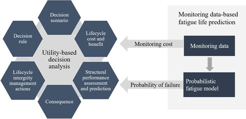
The methodology section introduces the principles of both utility-based decision analysis and monitoring data-based fatigue life predictions, which is shown in . The utility-based decision analysis solves the lifecycle integrity management problems considering structural performance assessment and prediction, consequences and lifecycle cost and benefit, with establishment of the decision scenarios and decision rules. The monitoring data-based fatigue life prediction provides input information for the utility-based decision analysis, such as monitoring costs and probability of fatigue failure based on a probabilistic fatigue model.
Figure 1. Road map of the proposed methodology.
2.1. Utility-based decision analysis
The utility theory dates back to 1738 when Bernoulli defined that the value of an object must not be determined on the basis of the price or cost, but instead on the utility it yields (Bernoulli, Citation1738). Inspired by Bernoulli’s hypothesis, Von Neumann et al. used it as a foundation to build their game theory in 1944, which is applicable to various contexts (Von Neumann, Morgenstern, & Kuhn, 2007). Furthermore, in 1961 Raiffa and Schlaifer formulated the decision theory (Raiffa & Schlaifer, Citation1961). This is now applied to the field of SHM and used for quantifying the value of monitoring information.
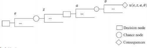
The decision process can be illustrated in a decision tree, as shown in . According to Raiffa and Schlaifer, a utility (monetary) function is assigned to a decision maker to describe the decision consequences when performing an experiment
e.g., a SHM strategy according to (Faber & Thöns, Citation2013; Pozzi & Der Kiureghian, Citation2011); observing a particular outcome
e.g., detecting damage or not; taking a particular action
e.g., repair, replace or do-nothing; and then obtaining a particular state of a structure
e.g., safe, damaged or failed. The utility function should contain the total cost and benefits throughout the decision process. The total cost will be the sum of the costs of consequences (failure costs considering fatalities, economic, environmental and social impacts); the cost of actions (e.g., repair cost); and the cost of monitoring (strain gauges investment, installation, operation and replacement costs, etc.). The benefits are related to the socio-economic effects for the state and company e.g., from toll charges and for the users, e.g., time saving and for the environment, e.g., from reduction of CO2 emissions.
Figure 2. Illustration of a decision tree.
However, the state of the structure is subjected to uncertainties. Therefore, a probability needs to be assigned to represent the belief of knowledge of the decision maker regarding the state of the structure
after implementing a strategy
obtaining the outcome
and taking an action
There may be
states in total for the structure, e.g., damaged, undamaged, slightly damaged or failed, etc. So that the expected utility
can be written as:
(1)
(1)
Depending on how much information is available at the time of decision making, the probabilities of the system states can be differentiated as prior probability when only the design information of the structure is known, posterior probability when additional SHM information is obtained and pre-posterior probability when SHM information is modelled and predicted but not yet implemented. The expected utility
will be termed accordingly as prior utility, posterior utility and pre-posterior utility (Faber, Citation2012).
When considering SHM, inspection and repair planning within the lifecycle integrity management, the expected utility during service life can be formulated as:
(2)
(2)
where:
where,
is the expected total lifecylce benifts,
is the expected total cost of failure during service life,
is the expected total lifecycle repair costs,
is the expected total inspection costs during service life,
is the expected total monitoring costs.
is the annual benefit at year
is the cost of failure at year
is the cost of repair at repair year
is the cost of inspection at inspection year
is the cost of monitoring at monitoring year
is the total number of repair,
is the total number of inspection,
is the total number of monitoring;
is the probability of failure at year
is the annual probability of failure at year
is the probability of repair at repair year
is the service life;
is the discounting rate. It is noted that a decision rule will normally be introduced to simplify the decision process, e.g. an action is required if the reliability reaches a specified target probability
The integrity management of a structure usually involves multiple choices of actions and SHM strategies. The optimal choice of action and SHM strategies is found through maximizing the expected utilities of different actions and SHM strategies during service life. The optimal action and strategy will result in the highest expected utility. In order to systematically analyse the expected utility influencing parameters beyond the probabilistic engineering models, the target probability benefit
failure cost
inspection costs
repair cost
monitoring cost
and discount rate
will be parametrically analysed in the frame of a posterior decision analysis in Section 4. The posterior probability of failure will be calculated using probabilistic data-based models described in Section 2.2.
2.2. Monitoring data-based fatigue life prediction
The monitoring data-based probabilistic model is built on three types of data as show in : pavement temperatures acquired from temperature sensors, vehicle traffic counts obtained from a toll system and strain data obtained from strain gauges. The following is a brief summary of the monitoring data-based probabilistic model as shown in , for a detailed and comprehensive model description it can be referred to (Farreras-Alcover, Chryssanthopoulos, & Andersen, Citation2017) .
Figure 3. Flow chart of monitoring data-based probabilistic model.
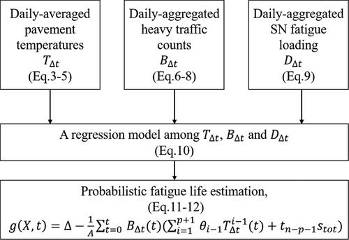
Table 1. Summary of the monitoring data from the monitoring system.
Fluctuations of the average of the pavement temperatures are modelled by a generic sinusoidal function with parameters
and
(3)
(3)
Daily-averaged pavement temperatures is de-seasonalized by deducting the daily mean value
and then differentiated by the monthly standard deviation
of the time series:
(4)
(4)
The de-seasonalized daily-averaged pavement temperature is further fitted to an autoregressive (AR) model, where
is the coefficient of AR model and
is a random normal error parameter at time t:
(5)
(5)
Similarly, the heavy daily-aggregated traffic count is firstly de-seasonalized to
by subtracting the daily average
and divided by the weekly standard deviation
of the time series:
(6)
(6)
A regression model is applied to identify the day-of-the-week effect on the de-seasonalized time series with the parameters
(ith regression coefficient),
(ith dummy descriptive variable) and
(random error process parameter at time t):
(7)
(7)
The traffic regression model’s residuals are modelled by an AR model where is the regression error at time t,
is the parameter of the AR model,
is the order of the AR model and
is a normal random error parameter:
(8)
(8)
The daily-aggregated fatigue loading at a given welded joint, is conservatively calculated from EquationEquation (9)
(9)
(9) , where
is the ith stress range out of the total amount of stress cycles
within the time step
(1 day) and
is the SN endurance curve slope:
(9)
(9)
In orthotropic steel decks, the key causes of fatigue damage are pavement temperatures and heavy traffic intensities. Hence, a regression model among daily-averaged pavement temperatures daily-aggregated heavy traffic counts
and daily-aggregated SN fatigue loading
is introduced by (Alcover, Citation2014). The left term in EquationEquation (10)
(10)
(10) can be regarded as normalized fatigue loading per heavy vehicle when considering SN curve with fatigue parameter
which is for simplification conservatively considered as single-slopped with no cut-off limit:
(10)
(10)
where
is a specified temperature of the pavement for which the forecast band is computed,
are the parameters of the regression model,
the number of data points corresponding to the training dataset associated used to approximate the regression parameters,
the order of the regression model,
a t-distribution with
degrees of freedom and
the estimate of the overall regression model variance at a given
The fatigue limit state function can be described on the basis of the SN curves to measure fatigue damage and with Miner's accumulation law:
(11)
(11)
where
is the random variables vector,
is Miner’s sum at failure (Miners Rule is one of the most used cumulative damage equations for failures caused by fatigue. When the sum of damage fractions is greater than 1.0, it will lead to failure),
is the material parameter defining the SN fatigue curve. Considering the above succession of regression and time-series models considering daily-averaged pavement temperatures and daily-aggregated heavy traffic, the limit state function of fatigue is:
(12)
(12)
The sensor measurement error could be further included in the probabilistic model define in EquationEquation (12)(12)
(12) . However, the measurement error has been found to be insignificant due to the quality of the installed equipment and its calibration in comparison to the other uncertainties (e.g., fatigue damage parameter A, Miner's sum at failure, etc.).
The weld will fail when the accumulated fatigue damage is larger than Miner’s sum at failure. So that the probability of failure can be estimated via Monte Carlo Simulation method as follows:
(13)
(13)
The uncertainties of the monitoring-based model are considered through modeling the SN fatigue parameter and Miner’s sum at failure as random variables not linked with SHM data. The uncertainties of the SHM data are treated on the process of deriving three different models for fatigue damage simulation: i) regression models for SN fatigue damage prediction (here the uncertainties are captured by the prediction bands of the models presenting described by in EquationEquation (10)
(10)
(10) , ii) time-series models for temperature prediction and iii) time-series models for traffic prediction. The uncertainties of the time-series models are captured by the random error process associated to each model and characterized via SHM data.
The pavement temperatures impact stress ranges on orthotropic steel decks and thereby influence fatigue life due to pavement-steel composite action. The model presented in EquationEquation (10)(10)
(10) predicts the fatigue damage at a given detail per unit of heavy vehicle and at a given pavement temperature. Then, EquationEquation (12)
(12)
(12) uses independent models for predicting heavy traffic counts and pavement temperatures. These models are eventually used to calculate fatigue damages. The results presented in the article correspond to a case with no increase of average pavement temperatures nor traffic levels than the ones used to derive the different data-based models. The probabilistic model for data-based fatigue life prediction used in EquationEquation (12)
(12)
(12) can consider different scenarios in terms of future average temperatures and traffic levels. This makes it possible to simulate unexpected events such as COVID-19 as they will have an impact on the daily number of heavy traffic vehicles used in the probabilistic model for fatigue prediction. In effect, vehicle counts and vehicle categories are monitored at the toll system of the bridge on an hourly basis; they have been used to characterize the traffic model
in EquationEquation (12)
(12)
(12) . More details can be found in (Farreras-Alcover et al., Citation2017).
3. Case study
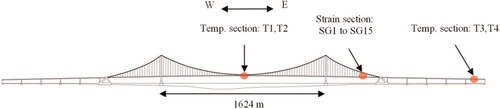
The above approach is illustrated with a case study from the Great Belt Bridge, which is a suspension bridge with main span of 1624 m and maximum hanger length of 177 m in Denmark as shown in . The cross-section of the orthotropic steel bridge deck (OSD) is formed with a closed steel box girder. Longitudinal troughs and crossbeams are located about 4 m apart on the OSD. The fatigue of through to deck weld and trough splice weld is considered with designed fatigue life of 100 years with certain fixed inspection intervals. Its operation started in 1998.
Figure 4. Illustration of Great Belt Bridge. (Temp. = Temperature, SG = Strain Gauge).
3.1. sHM system
In 2007, after approximately 10 years of operation, a comprehensive SHM system for design verification and condition monitoring was installed. The SHM system on the Great Belt bridge consists of, among others, a pavement temperature monitoring system, traffic monitoring system (used by the toll system) and strain monitoring system (). The location of the fatigue prone details to be assessed was determined prior to the writing of the article to perform a fatigue assessment task on the two critical details for the orthotropic steel deck under consideration: a trough-to-deck weld (detail category 50 according to EN1993-1-9-Part1-9) and a trough-splice weld (detail category 71 according to EN1993-1-9-Part1-9), as shown in . Details on the fatigue prediction methodology can be found in (Farreras-Alcover, Andersen, & McFadyen, Citation2016).
Figure 5. Illustration of strain monitoring system.

Figure 6. Strains gauges at welds (SG-TS = Strain Gauge Trough Splice, SG-TD: Strain Gauge Trough-to-deck).
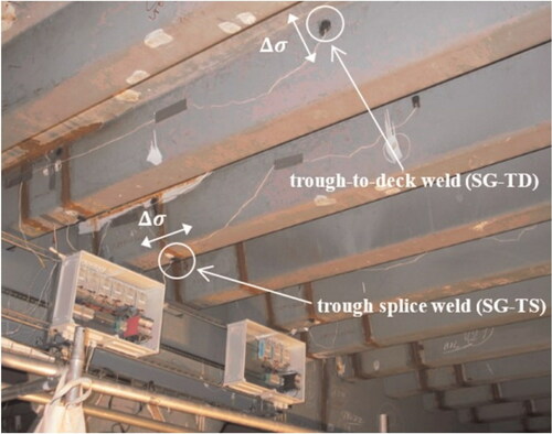
A cross-sectional strain monitoring system instrumented consists of 15 uniaxial strain gauges (), of which 10 gauges (i.e. 1,3,4,6,7,9,10,12,13,15) monitor the transverse nominal strains at the trough to deck weld, and 5 gauges (i.e. 2,5,8,11,14) monitor the longitudinal nominal strains at trough splice welds (). Strain gauges 1 to 9 are positioned under the slow traffic lane, which is passed by the heavy vehicles, while the others are positioned under the fast traffic lane. Four temperature monitoring sensors are embedded into two different cross-sections of the pavement and record the temperature every 5 minutes. At the tollgate, the crossing vehicles are immediately recorded on an hourly basis according to their measurements.
3.2. SHM strategies
Farreras-Alcover et al. concluded that the measurement from SG8 (measured the trough splice weld) were associated with the highest fatigue loading (Farreras-Alcover et al., Citation2016). This weld is under the slow traffic lane where heavy vehicles run inducing higher stress cycles than at the fast lane. For convenience of demonstration, the modelling of SHM strategies is based on the training data sets from SG8 between February 2012 to July 2012, which is assumed to capture the entire temperature spectrum within a normal year owing to the regular repeatability of the temperature spread on the pavement (Farreras-Alcover et al., Citation2016).
According to the different monitoring phases and the time duration, four different monitoring strategies in terms of time durations are discussed as presented in . The reference monitoring option represents continuous monitoring for 168 days, option
to option
represent periodical monitoring with two phases of separate monitoring and 7, 14, 28, 42 monitoring days per phase respectively. The time windows associated with 4 options are selected based on i) data availability and ii) consideration of representative 'extreme' weather conditions, i.e. data from February to July. In general, temperature variations are lower during cold conditions; hence this effect is accounted for in the calculated reliability profiles.
Table 2. SHM strategies.
3.3. Fatigue life prediction
The faituge life prediction is calculated following the probabilistic fatigue model from Section 2.2 and the variables in the probabilistic model are simulated following the model described in . The posterior probability of failure based on monitoring data for monitoring straetgy
is calculated with EquationEquation (13)
(13)
(13) and is shown in , which increases with time. For the purposes of this study, it is assumed that when reliability profiles reach a certain target probability, it is required to take a certain action. The target probability is set as 10−4 (reliability index β = 3.7) according to the Joint Committee on Structural Safety (JCSS, Citation2001) considering normal relative costs of safety measures and minor consequences of failure. The weld is assumed to get rehabilitation after reaching the target probability. The probability of repair at the repair year is equal to the target probability. After the rehabilitation, the welds are assumed to behave as new and the posterior failure probability is assumed to be the failure probability in the year zero. The total number of rehabilitations depends on how many times it will reach the target probability during the whole service life.
Figure 7. Prediction of probability of fatigue failure: (a) during service life of 120 years and with target probability (b) if doing nothing or rehabilitation given reference SHM data.
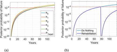
Table 3. Variables of the probabilistic model.
Let be the posterior probability of failure after the rehabilitation event
implemented at year
with SHM strategy
is the year in which the resulting posterior probability of failure
dependent on monitoring data from strategy
is equivalent to the target probability
The posterior probability of failure after rehabilitation
is calculated by:
(14)
(14)
The posterior probability of failure after rehabilitation given reference SHM data is shown in . It is worth noting that the fatigue reliability profiles are rather conservative considering single-slopped SN curves with no cut-off limit. The probabilistic models for the SN resistance are given in for the two details considered. A slope of m = 3 is considered for the SN curve in log-scale (number of cycles to failure versus stress range). The above assumptions highlight that the results presented in the article shall be read as an illustration of the presented methodology for assessing optimal monitoring strategies, and not as representative of the actual fatigue life of the instrumented details.
3.4. Decision scenario
As mentionend before the welds are designed with a fatigue life of 100 years. After obtaining the predictions for fatigue life based on monitoring data, for the purpose of the investigation presented in this article, it aims to explore whether to extend the service life of the welds to 120 years. Given that different monitoring strategies provide different predictions of fatigue reliability profiles, it aims to figure out which monitoring strategy can achieve maximum utilities/benefits for the lifecycle integrity management to rationalize the use of SHM techniques for fatigue assessment.
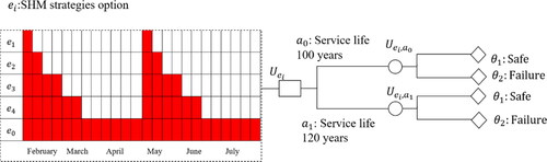
A utility-based decision analysis is introduced in section 2.1 to solve the problem. The decision process is visualised in with a decision tree where denoting the option of the actions, e.g.,
corresponding to a service life of 100 years and
to an extended service life of 120 years. For different choices of the service life, the integrity of the welds needs to be managed, which involves planned rehabilitation costs
The states of the welds
are defined as safe state
and failure state
which is effectively characterized by the fatigue reliability profiles. Welds will fail when the accumulated fatigue damage is larger than Miner’s damage at failure. If the weld stays safe, the bridge will be operated normally with annual benefits
If the weld fails, unscheduled rehabilitation events will be required, so that there will be a fatigue failure cost
which will be the unscheduled rehabilitation cost.
represents the different monitoring strategies from Section 3.2. Given the different monitoring phases and monitoring durations, there will be different costs of monitoring
Figure 8. Decision tree of posterior decision analysis.
3.5. Utility calculation
is to denote the expected maximum utilities regarding various actions with SHM strategy information
(15)
(15)
in which,
is the expected utility when the service life
is kept at 100 years (
) with monitoring option
is the expected utility when the service life
is extended to 120 years (
) with monitoring option
Let represent
and
(
), then the expected utility
of the SHM strategy information
for taking action
is calculated by:
(16)
(16)
It has to be noted that in EquationEquation (16)(16)
(16) , there is either
or
but not both in the same time;
is the annual benefit,
is the failure cost and
is the planned rehabilitation cost (in relation to EquationEquation (2)
(2)
(2) , repair costs
and inspection costs
are taken together in the case study and presented as rehabilitation cost
) ;
is the year of rehabilitation;
is the cost of monitoring per day;
is the total monitoring days from strategy
is the total number of repair times with action
is the year of monitoring.
is the discounting rate.
From the literature (Sund & Baelt, 2014), it is known that the Great Belt bridge and the connected tunnel, roads and railways together are called the Storebaelt link, which was built between 1988 and 1998, with the total construction costs amounting to EUR 3.56 billion in 1988 prices. The construction costs are financed through the state guarantee model and the loans are repaid by the users of the facilities. It is found that the Great Belt Company had loans guaranteed by the government and lent capital at an interest rate of 1.5-2% (Mouter, Citation2015). According to the report released by the Ministry of Transport and Sund & Baelt (2014), it is revealed that the Storebaelt link would bring a gain of EUR 50.87 billion over 50 years to Danish society, equivalent to EUR 1.21billion annually, while the construction and operation of the link over a 50 year period costs just EUR 18.66 billion.
Based on the information above, to illustrate the case study, it is assumed that half of the gain from the Storebaelt link comes from the Great Belt bridge, so that the normalized annual benefit for the Great Belt bridge is 0.17 (0.5*1.21/3.56) per year, the normalized cost of rehabilitation
is 5 (18.66/3.56), the normalized cost of failure
is assumed to be 100, the the normalized cost of monitoring
is assumed to be 0.01 per day, the discounting rate
is 0.02 (equavalent to interest rate) per year. It is noted that due to the confidentiality, the data shall be read as an illustration of the input paramenters of the presented methodology, and not as representative of the actual cost and benefits of the Great Belt bridge.
3.6. Results
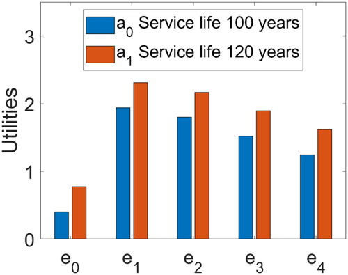
The utility calculation follows Section 3.5 and the results are shown in . The findings in indicate that for all SHM strategies it is recommended to extend service life to 120 years. The utilities in show that option will be recommended due to the highest utility. It is found that in the case study a long monitoring duration will reduce the risk but increase the cost of monitoring, which leads to an overall reduction in utility. The additional cost of longer monitoring is not justified here because the reduction of risk does not compensate for the increase of the cost. The optimal SHM strategy is thus short-term monitoring. However, the results may be sensitive to the variation of cost and benefit models, which is investigated in Section 4.
Figure 9. Identification on the most valuable SHM strategies during the bridge service life.
4. Parametric analysis
Further to the results presented in , due to the uncertainties related to the input parameters, a parametric analysis of the utilities associated with different monitoring durations and and choices of actions is performed considering the variability of the model parameters: (a) target probability (b) benefit
(c) failure cost
(d) reahbilitation cost
(e) monitoring cost
and (f) discount rate
4.1. Target probability 
The target probability is the acceptable optimum failure probability which is known as an adaptive control parameter based on the degree of failure impact and the relative expense of protection measures (JCSS, Citation2001). It varies from
(large consequences of failure, small relative cost of safety meausres) to
(minor consequences of failure and large relative cost safety meaure) according to (JCSS, Citation2001). The target probability
was previously chosen as
considering minor consequences of failure and a normal relative cost of safety measures. For assessing its effect, it is reduced from
to
and the outcomes are shown in . Reducing the target probability means that decision-makers are more conservative with lower tolerance of risk leading to the welds being rehabilitated more often during service life.
Figure 10. utilities associated with different monitoring durations and choices of actions considering the variability of the model parameters: (a) target probability (b) benefit
(c) failure cost
(d) inspection and rehabilitation cost
(e) monitoring cost
and (f) discount rate
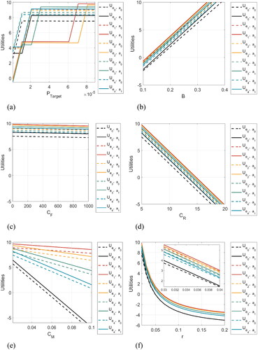
presents the utilities with the abovementioned change. The uitilies are all increasing with the increase of the target probability. It increases linearly in some ranges but stays constant in other ranges. The utilities curves of options and
with action
behave differently from the other curves. They start at the lowest value but end the highest values at the highest target probabilities. That’s because options
and
provide higher probability of failure than others. Hence, when
is high, options
and
will reach the target probability ealier, thus resulting in more times of rehabilitation when reaching 100 years
To compansate the increase of the rehabilitation costs, it will be suggested to continue operation to 120 years (
). Their flat plateau is however significantly lower than the plateaus of the other curves. The
action is more consistent with longer constant flat plateau over almost all of the observed range. For a low value of
all options except
and
have very similar utility values.
There are certain thresholds for where sudden increases of the utilities occur. When
option
with action
has the highest utility. When
utility with option
and action
is the highest. When
utility with option
and action
is the highest. When
option
with action
will be recommended. A summary of most valued decisions with changed of
can be found in . The summary of utilities in shows that the change of the target probability actively affect the decision of optimal SHM durations and service life extension of the welds. The tolerant- to- risk decision maker (high value of
) will get more benefit with the change on the
Table 4. Summary of the most valued decisions about the SHM strategy to adopt, regarding the critical parameters.
4.2. Benefit
The annual benefit is subjective to change due to the growth of population, change of urban planning etc. Therefore, the annual benefit rate is increased and the results are shown in . It is found that
has the highest utilities and the utilities associated with
extending service life to 120 years are always higher than those with
This is because of a higher profit-drive leading to a longer operation period. shows that the utilities increase linearly with the increase of benefit, but the difference between the slop of cures of the varied monitoring durations is very small.
4.3. Cost of failure
When increasing the cost of failure from 100 to 1000, the computation results in display the same trend as in leading to the extension to 120 years
with option
The utilities are slightly decreasing with the increase of
The choice of the service life extension and choice of monitoring duration are not influenced much by the change of cost of failure. It is because the difference between the utilities for 120 years and 100 years is the same. It is also due to the very small annual probability of failure, the accumulated risk of failure is comparably small as well.
4.4. Cost of rehabilitation
The cost of rehabilitation may be subject to change due to the choice of rehabilitation methods. When increasing the cost of rehabilitation from 5 to 50, the utilities in strongly decrease and become negative for both keeping the service life at 100 years
and extending it to 120 years
That is because the accumulated benefits and reduction of risk of failure cannot compensate the increase of cost of rehabilitations when the rehabilitation cost is too high. The variations between the maximum utilities of all the options in are very small. It can be interpreted that when the cost of rehabilitation is very high, it is no longer worthwhile to investigate the SHM strategies, which is not competitive, but the focus should be on finding solutions to reduce the cost of rehabilitations.
4.5. Cost of monitoring
The cost of monitoring may differ based on the choice of monitoring techniques. When increasing the cost of monitoring from 0.01 to 0.1 per day, shows that it is not beneficial to do monitoring with reference SHM option
due to high monitoring costs. As expected, the utility decreases with increasing monitoring durations, but the decreasing gradient is different. The curve of option
has the lowest gradient. Therefore, it is recommended to do monitoring with option
and extend the service life to 120 years. A decision-maker could learn that the sparser and shorter the SHM campagins, the better is the payback of monitoring and lesser its sensitive to the SHM cost.
4.6. Discounting rate
The discount rate is also connected with the so-called social discount rate, which represents the value that society assigns to its existing situation compared to potential future states. It has significant variations in practice around the world (Zhuang, Liang, Lin, & De Guzman, Citation2007), with lower levels introduced by developed countries (3%-7%) than the developing countries (8-15%). The value of discount rate also changes with time depending on public policies, e.g., the Danish Ministry of Finance in May 2013 reduced its social consumption discount rate from 5% per year to 4% per year for the first 35 years for the investment of long-term projects, 3% for the years in the interval 36 to 69 years, and 2% for the rest of years (Finansministeriet, Citation2013).
The discounting rate is increased from 0.02 to 0.2 and the results in illustrate that the utilities are exponentially decreasing and option
has the highest utilities. The utilities of keeping 100 years
or extending to 120 years
have almost the same value. When the discounting rate
is larger than 0.05, the utilities become negative. That’s because a higher discount rate means greater uncertainty and the cash flow in the future will have a lower value. Since money loses value fast with time, it is not beneficial to invest on long-term return projects. Thus it may be recommend not to invest in monitoring at all when the discounting rate
is high. A decision-maker could learn that the longer is the implementation of the SHM strategy, the higher the importance of the economic situation of the country.
5. Conclusions
Many studies focus on SHM data gathering, processing and probabilistic model developing. Building upon these studies, this article contains methodology to utilize the obtained monitoring information for the determination of i) optimal monitoring durations and ii) service life extension of the welds on a steel bridge deck. Through a posterior utility-based decision analysis of the welds on an orthotropic steel bridge deck case study, it is shown that a short-term SHM strategy has a higher expected utility and is thereby preferred. In contrast, long-term monitoring duration reduces the risks but leads to an increase of the monitoring costs, which in turn leads to an overall reduction in the expected utility.
Through a parametric analysis, this article shows how the target probability benefit
failure cost
rehabilitation cost
monitoring cost
and discounting rate
influence the expected value of the utility and thus the decisions:
It is found that the target probability
An increase of annual benefit
SHM strategies become not competitive (i.e., not worthwhile) when the cost of rehabilitation is too high. The rehablitation methods should be chosen carefully as a high rehabilitation cost
An increase of monitoring cost
For the investment in monitoring, the discounting rate
The presented research work considers solely the fatigue reliability and service life management of selected welds on an orthotropic steel bridge deck. Future research is needed to investigate the problem on a system level. Moreover, due to the methodology specificities, several assumptions on fatigue life prediction have been made and normalized cost and benefits models used. This highlights that the results presented in the article shall be read as an illustration of the presented methodology for assessing optimal monitoring strategies, and not necessarily as the actual fatigue life of the instrumented details and not as representative of the actual cost and benefits of the Great Belt bridge. Future research is envisaged to explore comprehensive probabilistic formulations of cost and benefit function and fatigue life prediction model considering not only a single slopped SN curve.
| Notations list | ||
| = | Utility function | |
| = | The SHM strategy/experiment | |
| = | The SHM /experiment outcome | |
| = | Action | |
| = | System state | |
| = | Probability of the state of the structure | |
| = | Expected utility function | |
| = | Expected utility during service life | |
| = | Expected benefit | |
| = | Expected cost of failure | |
| = | Expected cost of repair | |
| = | Expected cost of inspection | |
| = | Expected cost of monitoring | |
| = | The annual benefit at year | |
| = | The cost of failure at year | |
| = | The cost of repair at repair year | |
| = | The cost of inspection at inspection year | |
| = | The cost of monitoring at monitoring year | |
| = | The repair year | |
| = | The inspection year | |
| = | The monitoring year | |
| = | The total number of repair | |
| = | The total number of inspections | |
| = | The total number of monitoring | |
| = | The probability of failure at year | |
| = | The annual probability of failure at year | |
| = | The probability of repair at repair year | |
| = | The service life | |
| = | The discounting rate | |
| = | The target probability | |
| = | S-N fatigue loading aggregated during a time interval | |
| = | Daily aggregated counts of daily vehicles | |
| = | Daily averaged pavement temperature | |
| = | Estimator of the total variance of a regressing model | |
| = | Given pavement temperature | |
| = | Number of available datapoints | |
| = | Order of a polynomial regression model | |
| = | t-probability distribution with n-p-1 degrees of freedom | |
| = | Miner’s sum at failure | |
| = | Material parameter defining the SN fatigue curve. | |
Acknowledgements
This research was performed within the European project INFRASTAR (infrastar.eu), which has received funding from the European Union’s Horizon 2020 research and innovation program un-der the Marie Skłodowska-Curie grant agreement No 676139. The grant is gratefully acknowledged. Furthermore, the support of COST Action TU1402 on Quantifying the Value of Structural Health Monitoring is gratefully acknowledged. The authors would also like to thank Storebaelt A/S for allowing access to the monitored data from the Great Belt Bridge (Denmark) in the context of the present research. The authors would like to thank the anonymous reviewers and guest editors for the insightful and constructive review.
Disclosure statement
No potential conflict of interest was reported by the authors.
References
- Alcover, I. F. (2014). Data-based models for assessment and life prediction of monitored civil infrastructure assets [Doctoral dissertation]. University of Surrey. Retrieved from http://epubs.surrey.ac.uk/807811/.
- Balageas, D., Fritzen, C.-P., & Güemes, A. (2010). Structural health monitoring (Vol. 90). New Port Beach, CA, USA: John Wiley & Sons.
- Bayane, I., Long, L., Thöns, S., & Brühwiler, E. (2019). Quantification of the conditional value of SHM data for the fatigue safety evaluation of a road viaduct [Paper presentation]. 13th International Conference on Applications of Statistics and Probability in Civil Engineering (ICASP13), Seoul, South Korea. https://doi.org/10.22725/ICASP13.275.
- Bernoulli, D. (1738). Specimen theoriae novae de mensura sortis. Comentarii Academiae Scientarum Imperialis Petropolitanae (Vol. V, 1730–1731, published 1738) (pp. 175–192). Gregg.
- del Grosso, A. (2013). Structural health monitoring: Research and practice. [Paper presentation] Second Conference on Smart Monitoring, Assessment and Rehabilitation of Civil Structures -SMAR, Istanbul, Turkey.
- Diamantidis, D., Sykora, M., & Sousa, H. (2019). Quantifying the value of structural health information (SHI) for decision support - Guide for practising engineers (COST Action TU1402). Retrieved from https://www.cost-tu1402.eu/action/deliverables/guidelines.
- Eurocode. (2005). Eurocode 3: Design of steel structures—Part 1–9: Fatigue. European Committee for Standardization, Brussels.
- Faber, M. H. (2012). Bayesian decision analysis. In A.V. Gheorghe(Ed.), Statistics and probability theory: in pursuit of engineering decision support. (pp. 143–154). Springer Science & Business Media.
- Faber, M. H., & Thöns, S. (2013). On the value of structural health monitoring. In The 22nd Annual Conference on European Safety and Reliability (ESREL 2013), Amsterdam, The Netherlands.
- Farrar, C. R., & Worden, K. (2007). An introduction to structural health monitoring. Philosophical Transactions. Series A, Mathematical, Physical, and Engineering Sciences, 365(1851), 303–315. doi:https://doi.org/10.1098/rsta.2006.1928
- Farrar, C. R., & Worden, K. (2012). Structural health monitoring: A machine learning perspective. John Wiley & Sons, UK.
- Farrar, C. R., Sohn, H., Hemez, F. M., Anderson, M. C., Bement, M. T., Cornwell, P. J., & Robertson, A. (2003). Damage prognosis: Current status and future needs. Report. Los Alamos, NM: Los Alamos National Laboratory.
- Farreras-Alcover, I., Andersen, J. E., & McFadyen, N. (2016). Assessing temporal requirements for SHM campaigns. Proceedings of the Institution of Civil Engineers-Forensic Engineering, 169(2), 61–71. doi:https://doi.org/10.1680/jfoen.15.00015
- Farreras-Alcover, I., Chryssanthopoulos, M. K., & Andersen, J. E. (2017). Data-based models for fatigue reliability of orthotropic steel bridge decks based on temperature, traffic and strain monitoring. International Journal of Fatigue, 95, 104–119. doi:https://doi.org/10.1016/j.ijfatigue.2016.09.019
- Finansministeriet. (2013). Ny og lavere samfunds¯konomisk diskonteringsrate, Faktaark 31. (Ministry of Finance, 2013, New and lower socio-economic discount rate, Fact sheet 31).
- Flynn, E. B., & Todd, M. D. (2010). A Bayesian approach to optimal sensor placement for structural health monitoring with application to active sensing. Mechanical Systems and Signal Processing, 24(4), 891–903. doi:https://doi.org/10.1016/j.ymssp.2009.09.003
- Jcss, J. (2001). Probabilistic model code. Joint Committee on Structural Safety. https://www.jcss-lc.org/jcss-probabilistic-model-code/
- Long, L., Döhler, M., & Thöns, S. (2020). Determination of structural and damage detection system influencing parameters on the value of information. Structural Health Monitoring. 1475921719900918. doi:https://doi.org/10.1177/1475921719900918
- Long, L., Alcover, I. F., & Thöns, S. (2019). Quantification of the posterior utilities of SHM campaigns on an orthotropic steel bridge deck. In The Twelfth International Workshop on Structural Health Monitoring, Stanford, CA: Stanford University.
- Long, L., Thöns, S., & Döhler, M. (2018). The effects of SHM system parameters on the value of damage detection information. In EWSHM-9th European Workshop on Structural Health Monitoring, Manchester, UK.
- Mouter, N. (2015). Why do discount rates differ? Analyzing the differences between discounting policies for transport Cost-Benefit Analysis in five countries. Retrieved from http://www.mkba-informatie.nl/mkba-voorgevorderden/working-articles/mouter-why-do-discount-rates-differ-anayzlingdifferences-fi.
- Okasha, N. M., & Frangopol, D. M. (2012). Integration of structural health monitoring in a system performance based life-cycle bridge management framework. Structure and Infrastructure Engineering, 8(11), 1–1016. doi:https://doi.org/10.1080/15732479.2010.485726
- Orcesi, A. D., & Frangopol, D. M. (2011). Optimization of bridge maintenance strategies based on structural health monitoring information. Structural Safety, 33(1), 26–41. doi:https://doi.org/10.1016/j.strusafe.2010.05.002
- Pozzi, M., & Der Kiureghian, A. (2011). Assessing the value of information for long-term structural health monitoring. In Proceedings Volume 7984, Health Monitoring of Structural and Biological Systems 2011, SPIE Smart Structures and Materials + Nondestructive Evaluation and Health Monitoring, 2011, San Diego, CA. doi:https://doi.org/10.1117/12.881918
- Pozzi, M., Zonta, D., Wang, W., & Chen, G. (2010). A framework for evaluating the impact of structural health monitoring on bridge management. In D. Frangopol (Ed.), Bridge Maintenance, Safety, Management and Life-Cycle Optimization - Proceedings of the 5th International Conference on Bridge Maintenance, Safety and Management. IABMAS 2010, Philadelphia, PA.
- Qin, J., Thöns, S., & Faber, M. H. (2015). On the value of SHM in the context of service life integrity management. In Proceedings of the 12th International Conference on Applications of Statistics and Probability in Civil Engineering.
- Raiffa, H., & Schlaifer, R. (1961). Applied statistical decision theory. Wiley Classics Library.
- Sousa, H., Wenzel, H., & Thöns, S. (2019). Quantifying the Value of Structural Health Information (SHI) for Decision Support - Guide for operators (COST Action TU1402). Retrieved from https://www.cost-tu1402.eu/action/deliverables/guidelines.
- Sohn, H., Farrar, C. R., Hemez, F. M., Shunk, D. D., Stinemates, D. W., Nadler, B. R., & Czarnecki, J. J. (2003). A review of structural health monitoring literature: 1996–2001 (pp. 1–7). New Mexico: Los Alamos National Laboratory.
- Straub, D. (2014). Value of information analysis with structural reliability methods. Structural Safety, 49, 75–85. doi:https://doi.org/10.1016/j.strusafe.2013.08.006
- Sund & Baelt. (2014). The socio-economic importance of the Storebaelt link. Retrieved from http://publications.sundogbaelt.dk/Storeblt/the-socio-economic-importance-of-the-storebaelt-link/#/.
- Todd, M., Haynes, C., & Flynn, E. (2011). Bayesian experimental design approach to optimization in structural health monitoring. In Proceedings of World Congress on Advances in Structural Engineering and Mechanics.
- Thöns, S. (2019). Quantifying the Value of Structural Health Information (SHI) for decision support - guide for scientists (COST Action 1402). https://www.cost-tu1402.eu/action/deliverables/guidelines.
- Vanik, M. W., Beck, J. L., & Au, S. (2000). Bayesian probabilistic approach to structural health monitoring. Journal of Engineering Mechanics, 126(7), 738–745. doi:https://doi.org/10.1061/(ASCE)0733-9399(2000)126:7(738)
- Von Neumann, J., Morgenstern, O., Kuhn, W. H. (2007). Theory of games and economic behavior (Commemorative edition). Princeton University Press, UK.
- Wenzel, H., Veit-Egerer, R., Widmann, M., & To, I. (2011). Risk based civil SHM and life cycle management. In F. Chang (Ed.), Structural Health Monitoring 2011 Condition-Based Maintenance and Intelligent Structures (pp. 717–724). Destech Pubns Inc,USA.
- Wirsching, P. (1995). Probabilistic fatigue analysis. In Probabilistic structural mechanics handbook (pp. 146–165). Springer, Boston, MA.
- Zhuang, J., Liang, Z., Lin, T., & De Guzman, F. (2007). Theory and practice in the choice of social discount rate for cost-benefit analysis: A survey. In ADB Economics Working Paper Series. Asian Development Bank (ADB). https://www.econstor.eu/handle/10419/109296.
- Zonta, D., Glisic, B., & Adriaenssens, S. (2014). Value of information: Impact of monitoring on decision‐making. Structural Control and Health Monitoring, 21(7), 1043–1056. doi:https://doi.org/10.1002/stc.1631