Probabilistic analysis of the impact of climate change on creep of concrete structures in Sweden

Abstract

Recent studies suggest that concrete creep may be further exacerbated by climate change. However, up to now this effect has not been quantified in literature. The current study addresses this gap and presents a probabilistic approach for quantitatively assessing this effect. For this purpose, five different stochastic creep models (i.e. Model Code 1999, Model Code 2010, B3, B4, and B4s models) are used under considerations of the historical and future climatic conditions in Sweden to assess the long-term creep coefficient and the subsequent stress redistribution of an axially loaded column. While some creep models show similar percentage increases in the long-term creep coefficient in all Swedish counties, other creep models show higher percentage increase values for northern than for southern counties. The highest increase in the end-of-century creep coefficient is found using models B4 and B4s (e.g. over 40% increase is possible for northernmost Sweden, i.e. Norrbotten county, under RCP8.5). Furthermore, the current article also shows that the end-of-century creep coefficient is more sensitive to uncertainties not related to the climate (i.e. parameter and creep modelling uncertainties) than to climate uncertainty.

Keywords:

• climate change
• climate change uncertainty
• creep models
• creep model uncertainty
• long-term deformations
• stress redistribution

1. Introduction

It has now become evident that significant changes to the climate system are taking place (IPCC, 2021). Recent studies have identified several potential climate change impacts on infrastructure (Nasr, Björnsson, et al., 2021). According to the sixth assessment report (AR6) of the Intergovernmental Panel on Climate Change (IPCC), these impacts can significantly affect the performance and safety of many infrastructure elements (IPCC, 2022). Many of these impacts have been assessed in a quantitative manner; e.g. accelerated deterioration of infrastructure (Bastidas-Arteaga & Stewart, 2015b; Mortagi & Ghosh, 2022; Nasr, Honfi, & Larsson Ivanov, 2022; Nasr, Niklewski, Björnsson, & Johansson, 2022; Ryan & Stewart, 2021; Stewart, Wang, & Nguyen, 2011), increased scouring under submerged foundations of infrastructure (Kallias & Imam, 2016; Yang & Frangopol, 2019), and increased thermal stresses and displacements of infrastructure (Santillán, Salete, & Toledo, 2015). Nonetheless, many other identified potential impacts of climate change on infrastructure have not yet been investigated quantitatively. One of these impacts is the potential increase in creep of concrete structures due to climate change, see Nasr, Björnsson, et al. (2021).

Creep of concrete structures is in most cases regarded as a serviceability problem that may have impacts on maintenance and repair costs but cannot lead to structural collapse. However, several structural collapses during the past decades have been, at least partly, attributed to excessive creep deformations (Mazzotti & Buratti, 2021). For instance, the collapse of the Koror–Babeldaob Bridge in Palau in 1996 can be, at least partly, attributed to excessive creep deformations (Bažant, Hubler, & Yu, 2011). In Bažant et al. (2011) 56 other bridges were found to show similar problems with creep deformations and many more probably exist. Many models for assessing creep of concrete structures exist. Examples of these models are: Model Code 1999 model (MC99) (Eurocode model) (EN1992, 2004; FIB, 1999) which is an updated version of Model Code 1990 model (MC90) (Takács, 2002), Model Code 2010 model (MC10) (FIB, 2010), ACI model (ACI, 1992), GL 2000 model (Gardner & Lockman, 2001), MPF model (Chateauneuf, Raphael, & Moutou Pitti, 2014), B3 model (Bažant & Baweja, 2000), B4 model (Bažant, Hubler, & Wendner, 2015), and B4s model (Bažant et al, 2015). It has been noted earlier that some of the models commonly used in practice, e.g. MC99 model and ACI model, may grossly underestimate multi-decade creep, see, e.g. Bažant, Yu, and Li (2012). This highlights the large model uncertainty that characterises creep modelling.

Under this premise the aim of the current article is twofold. Firstly, the current article describes and demonstrates a probabilistic approach for quantifying the impact of climate change on creep of concrete structures and subsequent structural impacts (e.g. stress redistribution). Secondly, noting that the uncertainty related to climate change projections is often taken as an excuse for inaction to adapt to climate change impacts (Gifford, 2011), this article compares the effect of climate change uncertainty to the effect of uncertainties originating from other sources in assessing the impact of climate change on concrete creep, i.e. parameter uncertainty and creep model uncertainty. For this purpose, five different stochastic creep models (i.e. MC99, MC10, B3, B4, and B4s models) are applied under the historical and future climatic conditions in Sweden. It is shown that concrete creep is more sensitive to uncertainties not related to the climate (i.e. parameter and creep modelling uncertainties) than to climate uncertainty.

The article starts by describing the different creep models as well as their stochastic application (for the sake of brevity only two of the five models, i.e. MC99 and MC10, are presented in detail, the detailed description of the other three models can be found in the supplementary materials). A section that describes the climate model data used in the study then follows. The next section presents an illustrative example of an axially loaded column and assesses the impact of climate change on the long-term creep coefficient and the subsequent stress redistribution. Some important discussion points and further research directions are then presented. Lastly, the final section highlights some concluding remarks.

2. Creep modelling

As previously mentioned, there exist many models for predicting the creep behaviour of concrete structures. In the current study five different models are used: MC99, MC10, B3, B4, and B4s models. However, for the sake of brevity, this section only describes models MC99 and MC10. A detailed presentation of the other three models (B3, B4, and B4s models) can be found in the supplementary materials under section S1. Depending on the model used, creep of a concrete element at age $t$ due to a compressive stress $\sigma$ applied at age $t\prime$ is described by either the creep coefficient $\phi (t,t^{\prime })$ or the creep compliance $J(t,t\prime$). The relationship between $\phi (t,t^{\prime })$ and $J(t,t\prime$) is described by the following expression (Bažant et al, 2015): (1) $${\epsilon }_{\sigma }\left(t\right)=J\left(t,t^{\prime }\right)\sigma =\left(\frac{\phi (t,t^{\prime })+1}{E\left(t^{\prime }\right)}\right)\sigma$$(1) where ${\epsilon }_{\sigma }\left(t\right)$ is the stress-dependent strain (i.e. excluding shrinkage and thermal strains) at age $t$ and $E(t^{\prime })$ is the modulus of elasticity at loading age $t\prime .$

2.1. MC99 model (Eurocode model)

The MC99 model (EN1992, 2004; FIB, 1999) predicts $\phi (t,t^{\prime })$ as follows: (2) $$\phi \left(t,t^{\prime }\right)={\phi }_0{\beta }_c\left(t,t^{\prime }\right)$$(2) with: (3) $${\phi }_0={\phi }_{RH,T}\beta \left(f_{cm}\right)\beta \left(t^{\prime }\right)$$(3) (4) $${\mathrm{\phi }}_{RH,T}={\phi }_T+({\phi }_{RH}-1){{\phi }_T}^{1.2}$$(4) (5) $${\phi }_T=e^{0.015\left(T-20\right)}$$(5) (6) $${\phi }_{RH}=\left(1+\frac{1-\frac{RH}{100}}{0.1\sqrt[3]{h}}{\alpha }_1\right){\alpha }_2$$(6) (7) $${\alpha }_1={\left(\frac{35}{f_{cm}}\right)}^{0.7},\mathrm{ }{\alpha }_2={\left(\frac{35}{f_{cm}}\right)}^{0.2}$$(7) (8) $$\beta \left(f_{cm}\right)=\frac{16.8}{\sqrt{f_{cm}}}$$(8) (9) $$\beta \left(t^{\prime }\right)=\frac{1}{0.1+{\left({t^{\prime }}_{\mathit{adj}}\right)}^{0.2}}$$(9) (10) $${t\prime }_{\mathit{adj}}=t\prime {\left(\frac{9}{2+{\left(t^{\prime }\right)}^{1.2}}+1\right)}^{\alpha }\ge \mathrm{ }0.5\mathrm{ }\mathit{days}$$(10) (11) $$\alpha =\left\{\begin{array}{cc}-1& c\mathit{lass}\mathrm{ }32.5N\mathrm{ }(\mathit{class}\mathrm{ }S)\\ 0& c\mathit{lasses}\mathrm{ }32.5R,\mathrm{ }42.5N\mathrm{ }(\mathit{class}\mathrm{ }N)\\ 1& c\mathit{lasses}\mathrm{ }42.5R,\mathrm{ }52.5N,\mathrm{ }52.5R\mathrm{ }(\mathit{class}\mathrm{ }R)\end{array}\right\}$$(11) (12) $${\beta }_c\left(t,t^{\prime }\right)={\left(\frac{t-t^{\prime }}{{\beta }_{H,T}+(t-t^{\prime })}\right)}^{0.3}$$(12) (13) $${\beta }_{H,T}={\beta }_H{\beta }_T$$(13) (14) $${\beta }_H=1.5h\left(1+{\left(0.012RH\right)}^{18}\right)+250{\alpha }_3\le 1500{\alpha }_3$$(14) (15) $${\alpha }_3={\left(\frac{35}{f_{cm}}\right)}^{0.5}$$(15) (16) $${\beta }_{\mathrm{T}}=e^{\left(\frac{1500}{273+T}-5.12\right)}$$(16) where ${\phi }_0$ is the notional creep coefficient, ${\beta }_c\left(t,t^{\prime }\right)$ is the creep time development function, $T$ is the temperature in [°C], $RH$ is the relative humidity in [%], $h$ is the notional size of the concrete member in [mm], $f_{cm}$ is the mean compressive strength of concrete at the age of 28 days in [MPa], $t$ and $t\prime$ are the age and age at loading, respectively, in [days], ${t\prime }_{\mathit{adj}}$ is the adjusted age at loading based on cement type and $\alpha$ is a cement-type dependent factor.

The factors ${\phi }_T$ (Equation (5)(5) $${\phi }_T=e^{0.015\left(T-20\right)}$$(5) ) and ${\beta }_T$ (Equation (16)(16) $${\beta }_{\mathrm{T}}=e^{\left(\frac{1500}{273+T}-5.12\right)}$$(16) ) represent the effect of temperature on the notional creep coefficient and on the time development of creep, respectively. For a temperature of 20 °C (the default temperature of the model) both factors equal 1.0 and Equations (4)(4) $${\mathrm{\phi }}_{RH,T}={\phi }_T+({\phi }_{RH}-1){{\phi }_T}^{1.2}$$(4) and (13)(13) $${\beta }_{H,T}={\beta }_H{\beta }_T$$(13) reduce to the relative humidity dependent factors ${\phi }_{RH}$ and ${\beta }_H,$ respectively. It is worth noting that, the adjustment of the age at loading according to the curing temperature is not considered herein as this is not expected to be influenced by climate change. Furthermore, the transient creep coefficient that accounts for a sudden increase in temperature while the member is under load (e.g. due to fire) is not considered.

2.2. MC10 model

The MC10 model (FIB, 2010) predicts $\phi (t,t^{\prime })$ as follows: (17) $$\phi \left(t,t^{\prime }\right)={\phi }_{bc,T}\left(t,t^{\prime }\right)+{\phi }_{dc,T}\left(t,t^{\prime }\right)$$(17) with: (18) $${\phi }_{bc,T}\left(t,t^{\prime }\right)=\mathrm{ }{\phi }_{bc}\left(t,t^{\prime }\right){\phi }_T$$(18) (19) $${\phi }_{bc}\left(t,t^{\prime }\right)={\beta }_{bc}\left(f_{cm}\right){\beta }_{bc}\left(t,t\prime \right)$$(19) (20) $${\beta }_{bc}\left(f_{cm}\right)=\frac{1.8}{{f_{cm}}^{0.7}}$$(20) (21) $${\beta }_{bc}\left(t,t^{\prime }\right)=ln({(\frac{30}{{t^{\prime }}_{\mathit{adj}}}+0.035)}^2\left(t-t^{\prime }\right)+1)$$(21) (22) $${\phi }_{dc,T}\left(t,t^{\prime }\right)=\mathrm{ }{\phi }_{dc}\left(t,t^{\prime }\right){{\phi }_T}^{1.2}$$(22) (23) $${\phi }_{dc}\left(t,t^{\prime }\right)={\beta }_{dc}\left(f_{cm}\right)\beta \left(RH\right)\beta (t\prime ){\beta }_{dc}\left(t,t\prime \right)$$(23) (24) $${\beta }_{dc}\left(f_{cm}\right)=\frac{412}{{f_{cm}}^{1.4}}$$(24) (25) $$\beta \left(RH\right)=\frac{1-\frac{RH}{100}}{0.1\sqrt[3]{h}}$$(25) (26) $${\beta }_{dc}\left(t,t\prime \right)={\left(\frac{t-t^{\prime }}{{\beta }_{h,T}+(t-t^{\prime })}\right)}^{\gamma \left(t^{\prime }\right)}$$(26) (27) $$\gamma \left(t^{\prime }\right)=\frac{1}{2.3+\frac{3.5}{\sqrt{{t^{\prime }}_{\mathit{adj}}}}}$$(27) (28) $${\beta }_{h,T}={\beta }_h{\beta }_T$$(28) (29) $${\beta }_h=1.5h+250{\alpha }_3\le 1500{\alpha }_3$$(29) where ${\phi }_{bc,T}\left(t,t^{\prime }\right)$ and ${\phi }_{dc,T}\left(t,t^{\prime }\right)$ are the temperature adjusted basic creep (i.e. without moisture movement through the material) and drying creep coefficients, respectively, ${\phi }_{bc}\left(t,t^{\prime }\right)$ and ${\phi }_{dc}\left(t,t^{\prime }\right)$ are the basic creep and drying creep coefficients, respectively, ${\beta }_{bc}\left(t,t\prime \right)$ and ${\beta }_{dc}\left(t,t\prime \right)$ are the time development functions for basic and drying creep, respectively, and ${\phi }_T, f_{cm}, {t^{\prime }}_{\mathit{adj}}, \beta \left(t^{\prime }\right),$ ${\alpha }_3,$ $t$ and $t\prime$ are as defined in MC99 model description. Similar to MC99, the adjustment of the age at loading and the transient creep coefficients of MC10 are not considered in the context of this article.

2.3. Stochastic modelling of creep

This subsection describes the stochastic application of the presented creep models. For modelling the parameter uncertainty, the parameters $f_{cm}$ and $\mathrm{ }h$ are multiplied by the uncertainty factors ${\delta }_{f_{cm}}$ and ${\delta }_h,$ respectively. ${\delta }_{f_{cm}}$ and ${\delta }_h$ are represented by normal distributions with means of 1.0 and coefficients of variation (COV) of 0.15 (Bažant & Baweja, 2000) and 0.1 (Tu, Fang, Dong, & Frangopol, 2017), respectively.

For modelling the creep model uncertainty in MC99, Equation (2)(2) $$\phi \left(t,t^{\prime }\right)={\phi }_0{\beta }_c\left(t,t^{\prime }\right)$$(2) is multiplied with the model uncertainty factor ${\delta }_{MC99}$ (represented by a normal distribution with a mean of 1.0 and a COV of 0.47, see Wendner, Hubler, and Bažant (2015)). On the other hand, for modelling the creep model uncertainty in MC10, Equation (17)(17) $$\phi \left(t,t^{\prime }\right)={\phi }_{bc,T}\left(t,t^{\prime }\right)+{\phi }_{dc,T}\left(t,t^{\prime }\right)$$(17) is multiplied with the model uncertainty factor ${\delta }_{MC10}$ (represented by a normal distribution with a mean of 1.0 and a COV of 0.34, see Wendner et al. (2015)). It is acknowledged, however, that other distribution types and/or parameter values may be found in literature, see, e.g. Keitel and Dimmig-Osburg (2010).

3. Climate change scenarios and data

The Fifth Assessment Report (AR5) of the IPCC is based on four different climate change scenarios referred to as the Representative Concentration Pathway (RCP) scenarios (IPCC, 2013). In the current study, three of the four RCP scenarios are considered: RCP2.6, RCP4.5, and RCP8.5. Scenarios with forcings corresponding to these three scenarios are also adopted in the Sixth Assessment Report (AR6) of the IPCC in combination with the so-called Shared Socioeconomic Pathway (SSP) scenarios (i.e. SSP1-2.6, SSP2-4.5, and SSP5-8.5), see IPCC. (2021). The fourth RCP scenario (i.e. RCP6.0) is not considered herein due to data unavailability. However, the results of this scenario can be expected to broadly fall between those for scenarios RCP4.5 and RCP8.5. RCP2.6 is a relatively optimistic scenario in which stringent measures would be implemented to reduce greenhouse gas emissions (leading to a global mean temperature rise of 0.3–1.7 °C by the end of century) while RCP8.5 is a scenario with comparatively higher greenhouse gas emissions that result in a global mean temperature rise of 2.6–4.8 °C by the end of century.

RCP4.5 describes a future that is between the aforementioned two scenarios. Under the current state of knowledge, it is not possible to assign reliable probabilities to the different RCP scenarios (van Vuuren et al., 2011). As an example, while some studies conclude that exceeding RCP 8.5 has a probability of 12% (Capellán-Pérez, Arto, Polanco-Martínez, González-Eguino, & Neumann, 2016), the results of other studies contrastingly indicate that exceeding RCP 8.5 is economically impossible (Luke, 2018; Ritchie & Dowlatabadi, 2017). Hence, the plausibility of the different GHG emissions scenarios is still being debated in the scientific community and assigning explicit probabilities to these scenarios is considered unwarranted.

The climate data input to creep modelling is taken from the RCA4 regional climate model (Kjellstrom et al., 2016) operated over Europe at 50 × 50 km downscaled grid spacing. Aggregated data over each county in Sweden for the annual mean temperature and relative humidity is used. The climate change projections involve RCA4 downscaling five different global climate models (GCMs) under RCP2.6, RCP4.5, and RCP8.5. The considered GCMs are EC-EARTH, MIROC5, HadGEM2-ES, MPI-ESM-LR, and NorESM1-M. All GCMs have been used in the context of CMIP5 (the fifth phase of the coupled model intercomparison project), see Taylor, Stouffer, and Meehl (2012). For a more comprehensive description of the RCA4 climate projections see Kjellstrom et al. (2016). Although it is acknowledged that climate model outputs are subject to bias, the data used in the current study are not bias corrected. For bias adjusting relative humidity data, historical data of the relative humidity aggregated over the different counties is needed. Such data is not available.

Furthermore, it should be highlighted that serious doubts regarding the basis of existing bias correction methods and their application have been raised by several researchers, see, e.g. Ehret, Zehe, Wulfmeyer, Warrach-Sagi, and Liebert (2012) and Maraun et al. (2017). For instance, bias correction, generally, does not maintain the physical relations between the different climate variables. Due to the various problems characterising bias correction, many other studies that focused on analysing climate change impacts have used model projections that are not bias corrected, see, e.g. Alfieri, Burek, Feyen, and Forzieri (2015), Bell, Kay, Davies, and Jones (2016), Piotrowski, Osuch, and Napiorkowski (2021), and Sousa et al. (2020).

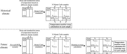
The procedure for considering the changing climate conditions in creep modelling is illustrated in Figure 1. The annual mean temperature and relative humidity data for each scenario were fitted to normal distributions for Monte Carlo simulation. These normal distributions reflect climate model uncertainty and inherent climate variability while scenario uncertainty is represented in the current article by considering different climate scenarios. For modelling creep under considerations of the historical climate (1961–1990), the average temperature and relative humidity in the historical period were used. For modelling creep under consideration of the future climate, the running average temperature and relative humidity at each time step were used.

Figure 1. Procedure for considering the changing climate conditions in creep modelling.

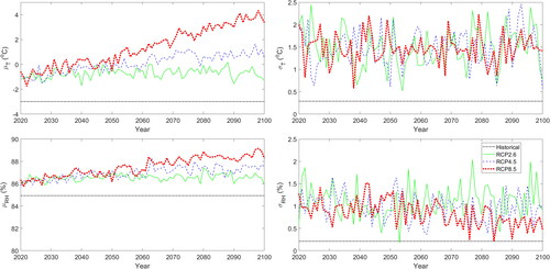
The mean and standard deviation of these normal distributions for the southernmost and northernmost counties (i.e. Skåne and Norrbotten) under the historical and future climate conditions are presented in Figures 2 and 3, respectively. These figures show that a clear increasing trend is observed for the annual average temperature in both counties (especially for RCP4.5 and RCP8.5). On the other hand, the relative humidity shows no clear trend for Skåne in all scenarios and an increasing trend for Norrbotten in RCP4.5 and RCP8.5 (although the increase is small compared to the increase in temperature).

Figure 2. Mean and standard deviation of the annual avearge temperature and relative humidity in Skåne based on the historical climate (1961–1990) and the three considered RCP scenarios; ${\mu }_T$ and ${\mu }_{RH}$ represent the mean value of the tempearture and relative humidty and ${\sigma }_T$ and ${\sigma }_{RH}$ represent the standard deviation of the tempearture and relative humidty, respectively.

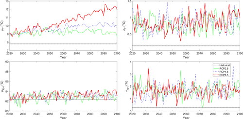
Figure 3. Mean and standard deviation of the annual avearge temperature and relative humidity in Norrbotten based on the historical climate (1961–1990) and the three considered RCP scenarios; ${\mu }_T$ and ${\mu }_{RH}$ represent the mean value of the tempearture and relative humidty and ${\sigma }_T$ and ${\sigma }_{RH}$ represent the standard deviation of the tempearture and relative humidty, respectively.

As in many previous studies, the current study adopts a probabilistic approach to generate random realisations of climate variables, see, e.g. Chateauneuf et al. (2014), Diamantidis, Madsen, and Rackwitz (1984), Guo, Sause, Frangopol, and Li (2011), Li and Melchers (1992), Merschman, Salman, Bastidas-Arteaga, and Li (2020), Mortagi and Ghosh (2022), and Ryan and Stewart (2021). The physical compatibility of annual average temperature and relative humidity pairs is ensured within the adopted climate models (i.e. RCA4 and each of the five GCMs). Considering the very small coefficient of variation of relative humidity projections (see Figures 2 and 3) and noting that for a certain value of annual average temperature, in any given location, a wide range of physically possible values of annual average relative humidity exists, using Monte Carlo simulation to generate random realisations of the two climate variables is very unlikely to result in physically incompatible pairs.

4. Illustrative example: effect of climate change on creep of an axially loaded column

4.1. Description

In this section, the effect of climate change on the creep coefficient and the subsequent stress redistribution of an axially loaded column is assessed. This section focuses on the climate conditions for two Swedish counties: 1) Skåne (the southernmost county) and 2) Norrbotten (the northernmost county). Results for the other Swedish counties can be found in the supplementary materials under section S2.

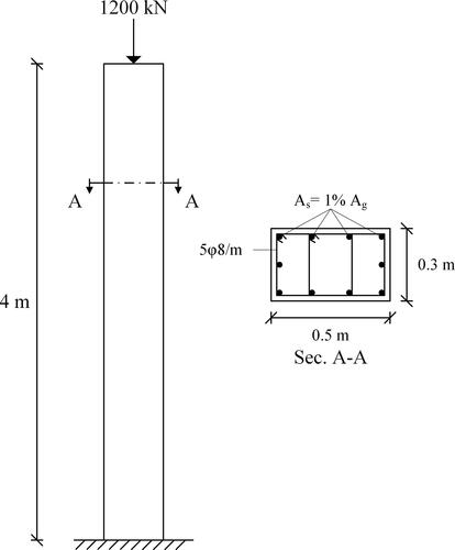
The considered column is adapted from an example presented in Samra (1995). The column, illustrated in Figure 4, has a cross section of 300 × 500 mm², is 4 m high, and is reinforced with 1% steel. The column is subjected to an axial load of 1200 kN. These four parameters are considered as deterministic variables. The following properties are assumed: 1) ASTM type I cement (corresponds to Class N, see Bažant et al. (2015)), 2) $t^{\prime }$ = 28 days, 3) $t_0$ = 28 days, 4) $f_{cm}$ = 27.6 MPa, 5) $h$ = 187.5 mm, 6) $c$ = 219.3 kg/m,³ 7) $\frac{w}{c}$ = 0.6, 8) $\frac{a}{c}$ = 7.0, 9) $\sigma$ = 8 MPa. While $h$ and $\sigma$ are based on the example in Samra (1995) the other properties are taken similar to the example in Bažant et al. (2015). The modulus of elasticity $E_s$ and yield strength $f_y$ of the reinforcement steel are taken as normally distributed random variables with mean values of 2 x 10⁵ MPa and 250 MPa and coefficients of variation (COV) of 0.03 and 0.1 respectively (distribution types and COV values are based on, e.g. Val, Stewart, and Melchers (1998)). The different parameters are assumed to be independent (i.e. uncorrelated).

Figure 4. The studied column; A_g and A_s represent the gross area of the column and the area of the longitudinal reinforcement, respectively.

It is assumed that the column is built in 2020, the curing is done in water, and the aggregate type is unknown. The column is exposed to evolving climate conditions over 81 years until the end of 2100. Relative humidity and temperature data for these 81 years according to the different RCP scenarios were used to assess the creep coefficient at 2100. Furthermore, the creep coefficient at 2100 was also assessed based on the historical (i.e. 1961–1990) climate data.

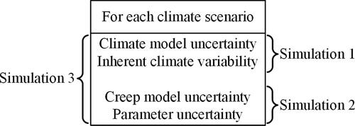
4.2. Effect on creep coefficient

For assessing the impact of climate change on creep, three Monte Carlo simulations (illustrated in Figure 5) were performed as follows: 1) considering only climate uncertainty (based on projections of five different climate models for each RCP scenario, see section 3), 2) considering only parameter and creep model uncertainty (based on the mean values of the temperature and relative humidity for each RCP scenario, see section 3), and 3) considering all involved uncertainties (climate uncertainty, parameter uncertainty, and creep model uncertainty). Climate uncertainty herein refers to climate model uncertainty and inherent climate variability while scenario uncertainty is represented through the consideration of different climate scenarios. These three simulations are performed to compare the effect of climate uncertainty to other uncertainty sources on the end-of-century creep coefficient. The end-of-century creep coefficient is considered herein as in the design of concrete structures the end-of-service creep coefficient is typically used. In these simulations, results of models B3, B4 and B4s were converted to $\phi (t,t^{\prime })$ using the relationship in Equation (1)(1) $${\epsilon }_{\sigma }\left(t\right)=J\left(t,t^{\prime }\right)\sigma =\left(\frac{\phi (t,t^{\prime })+1}{E\left(t^{\prime }\right)}\right)\sigma$$(1) .

Figure 5. Uncertainties considered in each Monte Carlo simulation.

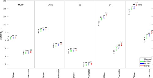
Figure 6 shows the resulting end-of-century creep coefficients in the first simulation using the different creep models under the different climatic conditions (i.e. historical, RCP2.6, RCP4.5, and RCP8.5) for Skåne and Norrbotten (see Figure S1 in the supplementary materials for the other counties). It can be observed that the creep coefficient in 2100 is higher for Skåne than for Norrbotten (and in general for southern than for northern counties) for all creep models. For instance, the median end-of-century creep coefficient using model B4s in RCP8.5 is ∼2.7 for Skåne and ∼2.0 for Norrbotten. Generally, model B4s results in the highest end-of-century creep coefficient, followed by models B4, MC10, MC99, and B3, respectively. For example, the median end-of-century creep coefficient in Skåne considering RCP8.5 is ∼2.7, ∼2.4, ∼2.1, ∼1.9, and ∼1.6 based on models B4s, B4, MC10, MC99, and B3, respectively. The results of all models show that the end-of-century creep coefficient is higher in RCP8.5 than in RCP4.5 than RCP2.6 than in the historical climate. The spread of each box in Figure 6 reflects the effect of climate model uncertainty and inherent climate variability on the end-of-century creep coefficient. On the other hand, for each creep model, the combined spread of the boxes representing the different climate scenarios for a certain county reflects the effect of the total climate projection uncertainty (i.e. scenario uncertainty, climate model uncertainty, and inherent climate variability) on the end-of-century creep coefficient.

Figure 6. Box plot of the end-of-century creep coefficients using the different creep models under the different climatic conditions (historical climate, RCP2.6, RCP4.5, and RCP8.5) considering only climate uncertainty for Skåne and Norrbotten.

Figures 7 and 8 present the resulting end-of-century creep coefficients in the second and third simulations, respectively, using the different creep models under the different climatic conditions (i.e. historical, RCP2.6, RCP4.5, and RCP8.5) for Skåne and Norrbotten (see Figures S2 and S3 in the supplementary materials for the other counties). Similar to Figure 6, the trend that southern counties have higher creep coefficients than northern counties can be observed. Compared to the results of simulation 1, see Figure 6, simulations 2 and 3 result in noticeably higher median end-of-century creep coefficients based on all models. For instance, the median end-of-century creep coefficient using model B4s in RCP8.5 in simulation 3 is ∼3.5 for Skåne and ∼2.6 for Norrbotten. The corresponding values in simulation 1 are ∼2.7 for Skåne and ∼2.0 for Norrbotten.

Figure 7. Box plot of the end-of-century creep coefficients using the different creep models under the different climatic conditions (historical climate, RCP2.6, RCP4.5, and RCP8.5) considering only parameter uncertainty and creep model uncertainty for Skåne and Norrbotten.

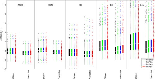
Figure 8. Box plot of the end-of-century creep coefficients using the different creep models under the different climatic conditions (historical climate, RCP2.6, RCP4.5, and RCP8.5) considering climate uncertainty, parameter uncertainty, and creep model uncertainty for Skåne and Norrbotten.

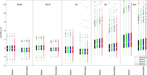
Moreover, similar to simulation 1, it can generally be observed that model B4s results in the highest end-of-century creep coefficient, followed by models B4, MC10, MC99, and B3, respectively. The results of all models show that the end-of-century creep coefficient is higher in RCP8.5 than in RCP4.5 than RCP2.6 than in the historical climate for all counties. For each climate scenario, the spread of each box in Figure 7 reflects the effect of parameter and creep model uncertainty on the end-of-century creep coefficient while the spread of each box in Figure 8 represents the effect of all involved uncertainties.

Comparing Figures 6–8, an important observation is that the variability of the end-of-century creep coefficient is much larger in simulations 2 and 3 than in simulation 1. For instance, the 25^th and 75^th percentiles of the end-of-century creep coefficient in Skåne based on model B4s in RCP8.5 are ∼2.7 and ∼2.71, respectively, in simulation 1 and ∼2.25 and ∼5.54, respectively, in simulation 3. The much larger spread of the results in simulations 2 and 3 compared to simulation 1 indicates that parameter uncertainty and creep model uncertainty have a considerably larger effect on the end-of-century creep coefficient than climate uncertainty (even when scenario uncertainty is considered).

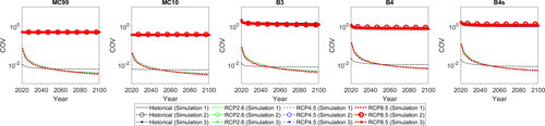
Figures 9 and 10 further highlight that the end-of-century creep coefficient is more sensitive to uncertainties not related to the climate (i.e. parameter and creep modelling uncertainties) than to climate uncertainty. Figures 9 and 10 show the COV of the creep coefficient in simulations 1–3 using the different creep models under the different climatic conditions (i.e. historical, RCP2.6, RCP4.5, and RCP8.5) for Skåne and Norrbotten, respectively. All models show that the COV in simulations 2 and 3 is very similar and is much larger than in simulation 1. For simulation 1, the COV of the creep coefficient shows a decreasing trend in all RCP scenarios and is almost constant with time in the historical climate for both Skåne and Norrbotten. For simulations 2 and 3, the COV of the creep coefficient is almost constant with time in all climatic conditions for both counties.

Figure 9. Coefficient of variation of the creep coefficient using the different creep models under the different climatic conditions (historical climate, RCP2.6, RCP4.5, and RCP8.5) in simulations 1-3 for Skåne.

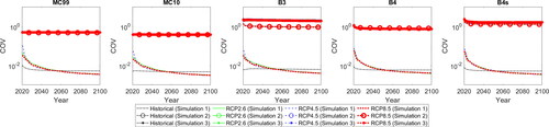
Figure 10. Coefficient of variation of the creep coefficient using the different creep models under the different climatic conditions (historical climate, RCP2.6, RCP4.5, and RCP8.5) in simulations 1-3 for Norrbotten.

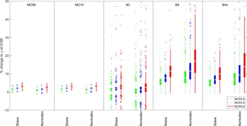
Figure 11 depicts the percentage change in the end-of-century creep coefficients in the different RCP scenarios compared to the historical climate using the different creep models and considering all involved uncertainties (i.e. simulation 3) for Skåne and Norrbotten (see Figure S4 in the supplementary materials for the other counties). Models MC99, MC10, and B3 result in similar percentage increase values with median values not higher than ∼2% in RCP2.6, ∼2.5% in RCP4.5, and ∼3.5% in RCP8.5. On the other hand, models B4 and B4s show significantly higher percentage increase values than the other three models with a visible trend of higher percentage increase values in northern than in southern counties, see Figure S4. For instance, based on these two models, over 40% increase is possible for Norrbotten in RCP8.5 while the highest increase in Skåne is slightly over 20% in the same scenario.

Figure 11. Box plot of the percentage change in the end-of-century creep coefficients in the different RCP scenarios compared to the historical climate using the different creep models considering climate uncertainty, parameter uncertainty, and creep model uncertainty for Skåne and Norrbotten.

4.3. Effect on stress redistribution

In reinforced concrete sections, stress redistribution between the concrete and the reinforcement occurs due to creep. In axially loaded columns, the direction of this transfer is normally from the concrete to the reinforcing steel and hence the concrete stress is gradually reduced with time while the stress of the reinforcement steel is gradually increased (Samra, 1995). In this subsection, the effect of creep on the stress redistribution of the studied column is assessed for Skåne and Norrbotten under the different climatic conditions (i.e. historical, RCP2.6, RCP4.5, and RCP8.5) considering all involved uncertainties (i.e. simulation 3 in the previous section). For this purpose, the approach developed by Samra (1995) for analysing the creep behaviour in reinforced concrete columns is used.

In Samra (1995) the concrete stress at time $t$ is assessed as follows: (30) $${\sigma }_{ct}={\sigma }_{ci}\left(\frac{\left(1-{\rho }_s\right)+n\left(1-0.2\phi \left(t,t^{\prime }\right)\right){\rho }_s}{\left(1-{\rho }_s\right)+n\left(1+0.8\phi \left(t,t^{\prime }\right)\right){\rho }_s}\right)$$(30) where ${\sigma }_{ct}$ is the concrete stress at time $t,$ ${\sigma }_{ci}$ is the initial concrete stress, ${\rho }_s$ is the steel ratio with respect to the gross cross section, and $n$ is the modular ratio (i.e. the ratio of the modulus of elasticity of the reinforcement steel to that of the concrete). The steel stress at time $t$ is assessed as follows (Samra, 1995): (31) $${\sigma }_{st}={n\sigma }_{ci}\left(0.2\phi \left(t,t^{\prime }\right)+\frac{{\sigma }_{ct}}{{\sigma }_{ci}}\left(1+0.8\phi (t,t^{\prime })\right)\right)$$(31) where ${\sigma }_{st}$ is the reinforcement steel stress at time $t.$ The initial concrete stress ${\sigma }_{ci}$ and the initial steel stress ${\sigma }_{si}$ are calculated as follows: (32) $${\sigma }_{ci}=\frac{F}{A_c+n{A}_s}$$(32) (33) $${\sigma }_{si}=n{\sigma }_{ci}$$(33) where $F$ is the applied axial load, $A_c$ is the area of concrete, and $A_s$ is the area of steel.

Figures 12 and 13 display the probability that the reinforcement steel reaches its yield strength over time for Skåne and Norrbotten, respectively, using the different creep models under the different climatic conditions (i.e. historical, RCP2.6, RCP4.5, and RCP8.5). Significant differences are observed between the results of the different models. For instance, the probability of reaching a steel stress that is equal to or higher than the yield strength at the end of the century in RCP8.5 for Skåne varies from ∼0.028 based on MC10 to ∼0.4 based on model B4s. The corresponding range for Norrbotten is from ∼0.0056 based on MC10 to ∼0.26 based on model B4s. Furthermore, the percentage increases in this probability compared to the historical climate also varies significantly across models.

Figure 12. The probability that the reinforcement steel reaches its yield strength over time using the different creep models for Skåne.

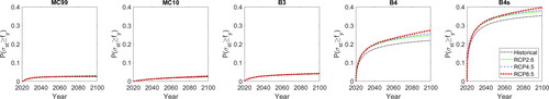
Figure 13. The probability that the reinforcement steel reaches its yield strength over time using the different creep models for Norrbotten.

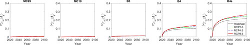
For example, the percentage increases for Skåne in RCP8.5 varies between ∼8.4% based on model B3 to ∼25.1% based on model B4. The corresponding range for Norrbotten is from ∼3.9% in model B3 to ∼37.4% in model B4. The results in Figures 12 and 13 show that the uncertainty related to creep modelling has a much larger effect on the probability of reinforcement yielding than climate uncertainty (which includes scenario uncertainty, climate model uncertainty, as well as inherent climate variability).

5. Discussion and further research

Considering the results in the previous section, it is evident that the end-of-century creep coefficient is more sensitive to uncertainties not related to the climate (i.e. parameter and creep modelling uncertainties) than to climate uncertainty. This finding is consistent with the results of other studies that addressed other potential climate change impacts on infrastructure, e.g. scour under submerged bridge foundations (Kallias & Imam, 2016) and atmospheric corrosion of steel structures (Nguyen, Wang, & Leicester, 2013). Noting that these non-climatic uncertainties have always existed and have been successfully dealt with by the engineering community (as evidenced by the fact that most concrete structures have satisfactory performances with regard to creep), climate uncertainty should not be taken as an excuse for inaction to adapt our infrastructure to the impacts of climate change. It is interesting to note that, even when modelling uncertainties are included in the analysis large differences are still observed between the different models. It should be noted, however, that in Wendner et al. (2015) models B4 and B4s, which show the highest climate change impact on creep of concrete structures, were found to be the most accurate of all considered models followed by MC10, B3, and MC99, respectively.

A viable future research direction is to investigate the impact of climate change on concrete creep using other models which may be more comprehensive (as the uncertainty associated with these models may be less than that associated with the adopted models), see, e.g. Sellier et al. (2016). In addition, investigating the effect of parameter correlation in the current context is worthy of attention. However, previous research found that this effect is comparatively small for models MC99 and B3 when creep model uncertainty is considered (Keitel & Dimmig-Osburg, 2010). Additionally, it is worth highlighting that the current study, as well as most studies investigating the impacts of climate change on infrastructure (see, e.g. Bastidas-Arteaga and Stewart (2015a, 2015b), Merschman et al. (2020), Peng and Stewart (2014a, 2014b), Ryan and Stewart (2021), Stewart et al. (2011), Yang and Frangopol (2019), and Zhang, Ayyub, and Fung (2022)), do not focus on a specific structure but rather they aim at quantifying the impact of climate change on a county, city, or watershed level. Assessing the impact of climate change on a specific structure would require climate data that are produced at a significantly finer resolution than that used in these studies (the finest grid resolution in the previous studies is 8 × 8 km in Bastidas-Arteaga and Stewart (2015a)). Such data is not readily available for most locations (Nasr, Björnsson, et al., 2021). However, as the modelling in the current study depends on average annual values of temperature and relative humidity, the resolution of climate data is not expected to significantly alter the results.

Further research should aim at assessing other effects of creep on the structural behaviour of concrete structures in light of a changing climate, see, e.g. Rüsch, Jungwirth, and Hilsdorf (1983). Examples of other structural effects related to creep are loss of prestressing forces in prestressed elements (Chateauneuf et al., 2014), induced bending stresses on the piles of integral abutment bridges (Arockiasamy, Butrieng, & Sivakumar, 2004), and differential column shortening in high-rise buildings (Moragaspitiya, Thambiratnam, Perera, & Chan, 2010). Furthermore, the impact of climate change on shrinkage and thermal strains should be assessed and added to the creep strain. Lastly, the combined effect of creep and other potential climate change impacts on concrete structures, e.g. deterioration of concrete structures (Nasr, Honfi, et al., 2022; Stewart et al., 2011), is worthy of investigation.

6. Conclusions

Climate change can impact the safety and performance of infrastructure in many aspects. One of the impacts that have not been quantitatively assessed so far is the impact of climate change on creep of concrete structures. This article addresses this gap by proposing and demonstrating a probabilistic approach for quantifying the impact of climate change on creep of concrete structures and subsequent structural impacts (e.g. stress redistribution). For this purpose, the impact of climate change on long-term creep and the subsequent stress redistribution of an axially loaded column is assessed using five different creep models (i.e. models MC99, MC10, B3, B4, and B4s) under the Swedish climate conditions.

The highest increase in the end-of-century creep coefficient is found using models B4 and B4s. Based on these two models, for instance, over 40% increase in the end-of-century creep coefficient in RCP8.5 is possible for Norrbotten (northernmost county in Sweden) in comparison to the historical climate. These two models also show higher percentage increase values for northern than for southern Swedish counties. For instance, based on these two models, the highest increase in Skåne (southernmost county in Sweden) is slightly over 20% in RCP8.5 (compared with over 40% for Norrbotten). The other three models (i.e. MC99, MC10, and B3) show percentage increases in the long-term creep coefficient which are significantly less than those observed for models B4 and B4s. For instance, the highest increases in the end-of-century creep coefficient in Norrbotten in RCP8.5 are in the vicinity of 4.5%, 5%, and 11% based on models MC99, MC10, and B3, respectively. The corresponding values for Skåne are 4.6%, 4.6%, and 7.2%, respectively.

The current article also shows that the end-of-century creep coefficient is more sensitive to uncertainties not related to the climate (i.e. parameter and creep modelling uncertainties) than to climate uncertainty. This finding is consistent with the results of other studies that addressed other potential climate change impacts on infrastructure, e.g. scour under submerged bridge foundations and atmospheric corrosion of steel structures. Noting that these non-climatic uncertainties have always existed and have been successfully dealt with by the engineering community (as evidenced by the fact that most concrete structures have satisfactory performances with regard to creep), climate uncertainty should not be taken as an excuse for inaction to adapt our infrastructure to the impacts of climate change.

Acknowledgements

Erik Kjellström and Gustav Strandberg from SMHI are acknowledged for providing the climate model projections. Dániel Honfi from Stockholms Stad transport department, Erik Kjellström from SMHI, Ivar Björnsson and Jonas Johansson from Lund University, and Oskar Larsson Ivanov from Boverket are acknowledged for their invaluable comments and support. The author also thanks four anonymous reviewers whose comments greatly enhanced the quality of the article. Any opinions, findings, or conclusions stated herein are those of the author and do not reflect the opinions of the financiers nor of any other individual.

Disclosure statement

No potential conflict of interest was reported by the author.

Additional information

Funding

The author gratefully acknowledges the financial support provided by the Swedish Transport Administration [grant numbers 2016-008 & 2019-027] and the strategic innovation program InfraSweden2030 [grant number 2018-00611], a joint effort of Sweden’s Innovation Agency (Vinnova), the Swedish Research Council (Formas) and the Swedish Energy Agency (Energimyndigheten).

References

- ACI. (1992). Prediction of creep, shrinkage and temperature effects in concrete structures ACI 209R-92 (minor update of original 1971 version). Farmington Hills, MI: American Concrete Institute.
- Alfieri, L., Burek, P., Feyen, L., & Forzieri, G. (2015). Global warming increases the frequency of river floods in Europe. Hydrology and Earth System Sciences, 19(5), 2247–2260. doi:10.5194/hess-19-2247-2015
- Arockiasamy, M., Butrieng, N., & Sivakumar, M. (2004). State of the art of integral abutment bridges: Design and practice. Journal of Bridge Engineering, 9(5), 497–506. doi:10.1061/(ASCE)1084-0702(2004)9:5(497)
- Bastidas-Arteaga, E., & Stewart, M. G. (2015a). Damage risks and economic assessment of climate adaptation strategies for design of new concrete structures subject to chloride-induced corrosion. Structural Safety, 52, 40–53. doi:10.1016/j.strusafe.2014.10.005
- Bastidas-Arteaga, E., & Stewart, M. G. (2015b). Economic assessment of climate adaptation strategies for existing reinforced concrete structures subjected to chloride-induced corrosion. Structure and Infrastructure Engineering, 12(4), 432–449. doi:10.1080/15732479.2015.1020499
- Bažant, Z. P., & Baweja, S. (2000). Creep and shrinkage prediction model for analysis and design of concrete structures: Model B3. In The Adam Neville Symposium: Creep and Shrinkage—Structural Design Effects, Farmington Hills, MI, USA.
- Bažant, Z. P., Hubler, M. H., & Wendner, R. (2015). RILEM draft recommendation: TC-242-MDC multi-decade creep and shrinkage of cocrete: material model and structural analysis—Model B4 for creep, drying shrinkage and autogenous shrinkage of normal and high-strength concretes with multi-decade applicability. Materials and Structures, 48, 753–770.
- Bažant, Z. P., Hubler, M. H., & Yu, Q. (2011). Pervasiveness of excessive segmental bridge deflections: Wake-up call for creep. ACI Structural Journal, 108(6), 766–774.
- Bažant, Z. P., Yu, Q., & Li, G.-H. (2012). Excessive long-time deflections of prestressed box girders. II: Numerical analysis and lessons learned. Journal of Structural Engineering, 138(6), 687–696. doi:10.1061/(ASCE)ST.1943-541X.0000375
- Bell, V. A., Kay, A. L., Davies, H. N., & Jones, R. G. (2016). An assessment of the possible impacts of climate change on snow and peak river flows across Britain. Climatic Change, 136(3–4), 539–553. doi:10.1007/s10584-016-1637-x
- Capellán-Pérez, I., Arto, I., Polanco-Martínez, J. M., González-Eguino, M., & Neumann, M. B. (2016). Likelihood of climate change pathways under uncertainty on fossil fuel resource availability. Energy & Environmental Science, 9(8), 2482–2496. doi:10.1039/C6EE01008C
- Chateauneuf, A. M., Raphael, W. E., & Moutou Pitti, R. J. B. (2014). Reliability of prestressed concrete structures considering creep models. Structure and Infrastructure Engineering, 10(12), 1595–1605. doi:10.1080/15732479.2013.835831
- Diamantidis, D., Madsen, H. O., & Rackwitz, R. (1984). On the variability of the creep coefficient of structural concrete. Matériaux et Constructions, 17(4), 321–328. doi:10.1007/BF02479090
- Ehret, U., Zehe, E., Wulfmeyer, V., Warrach-Sagi, K., & Liebert, J. (2012). Should we apply bias correction to global and regional climate model data? Hydrology and Earth System Sciences, 16(9), 3391–3404. doi:10.5194/hess-16-3391-2012
- EN1992. (2004). Eurocode 2-design of concrete structures – Part 1-1: General rules and rules for buildings. Part 2: Concrete bridges. Brussels, Belgium: European Committee for Standardization.
- FIB. (1999). Structural concrete: Textbook on behaviour, design and performance, updated knowledge of the CEB/FIP model Code 1990, Bulletin No. 2. Lausanne, Switzerland: Federation internationale du beton (FIB).
- FIB. (2010). Model code 2010. Lausanne, Switzerland: Federation internationale du beton.
- Gardner, N. J., & Lockman, M. J. (2001). Design provisions of shrinkage and creep of normal-strength concrete. ACI Materials Journal, 98, 159–167.
- Gifford, R. (2011). The dragons of inaction: Psychological barriers that limit climate change mitigation and adaptation. The American Psychologist, 66(4), 290–302. 10.1037/a0023566.
- Guo, T., Sause, R., Frangopol, D. M., & Li, A. (2011). Time-dependent reliability of PSC box-girder bridge considering creep, shrinkage, and corrosion. Journal of Bridge Engineering, 16(1), 29–43. doi:10.1061/(ASCE)BE.1943-5592.0000135
- IPCC. (2013). Climate change 2013: The physical science basis – Contribution of Working Group I to the Fifth Assessment Report of the Intergovernmental Panel on Climate Change. Cambridge & New York: Cambridge University Press.
- IPCC. (2021). Climate change 2021: The physical science basis. Contribution of Working Group I to the Sixth Assessment Report of the Intergovernmental Panel on Climate Change. Cambridge & New York: Cambridge University Press.
- IPCC. (2022). Climate Change 2022: Impacts, adaptation, and vulnerability-Working Group II contribution to the Sixth Assessment Report of the Intergovernmental Panel on Climate Change. Cambridge & New York: Cambridge University Press.
- Kallias, A. N., & Imam, B. (2016). Probabilistic assessment of local scour in bridge piers under changing environmental conditions. Structure and Infrastructure Engineering, 12(9), 1228–1241. doi:10.1080/15732479.2015.1102295
- Keitel, H., & Dimmig-Osburg, A. (2010). Uncertainty and sensitivity analysis of creep models for uncorrelated and correlated input parameters. Engineering Structures, 32(11), 3758–3767. doi:10.1016/j.engstruct.2010.08.020
- Kjellstrom, E., Barring, L., Nikulin, G., Nilsson, C., Persson, G., & Strandberg, G. (2016). Production and use of regional climate model projections – A Swedish perspective on building climate services. Climate Services, 2-3, 15–29. 10.1016/j.cliser.2016.06.004.
- Li, C. Q., & Melchers, R. E. (1992). Reliability analysis of creep and shrinkage effects. Journal of Structural Engineering, 118(9), 2323–2337. doi:10.1061/(ASCE)0733-9445(1992)118:9(2323)
- Luke, A. (2018). Preparing for what? Design floods and environmental change [Doctoral dissertation]. University of California Irvine. https://escholarship.org/uc/item/4m2428qd.
- Maraun, D., Shepherd, T. G., Widmann, M., Zappa, G., Walton, D., Gutiérrez, J. M., Hagemann, S., Richter, I., Soares, P. M. M., Hall, A., & Mearns, L. O. (2017). Towards process-informed bias correction of climate change simulations. Nature Climate Change, 7(11), 764–773. doi:10.1038/nclimate3418
- Mazzotti, C., & Buratti, N. (2021). A design oriented fibre-based model for simulating the long-term behaviour of RC beams: Application to beams cast in different stages. Journal of Building Engineering, 44, 103176. doi:10.1016/j.jobe.2021.103176
- Merschman, E., Salman, A. M., Bastidas-Arteaga, E., & Li, Y. (2020). Assessment of the effectiveness of wood pole repair using FRP considering the impact of climate change on decay and hurricane risk. Advances in Climate Change Research, 11(4), 332–348. doi:10.1016/j.accre.2020.10.001
- Moragaspitiya, P., Thambiratnam, D., Perera, N., & Chan, T. (2010). A numerical method to quantify differential axial shortening in concrete buildings. Engineering Structures, 32(8), 2310–2317. doi:10.1016/j.engstruct.2010.04.006
- Mortagi, M., & Ghosh, J. (2022). Concurrent modelling of carbonation and chloride-induced deterioration and uncertainty treatment in aging bridge fragility assessment. Structure and Infrastructure Engineering, 18(2), 197–218. doi:10.1080/15732479.2020.1838560
- Nasr, A., Björnsson, I., Honfi, D., Larsson Ivanov, O., Johansson, J., & Kjellström, E. (2021). A review of the potential impacts of climate change on the safety and performance of bridges. Sustainable and Resilient Infrastructure, 6(3–4), 192–212. doi:10.1080/23789689.2019.1593003
- Nasr, A., Honfi, D., & Larsson Ivanov, O. (2022). Probabilistic analysis of climate change impact on chloride-induced deterioration of reinforced concrete considering Nordic climate. Journal of Infrastructure Preservation and Resilience, 3(1), 1–16. doi:10.1186/s43065-022-00053-6
- Nasr, A., Larsson Ivanov, O., Björnsson, I., Johansson, J., & Honfi, D. (2021). Towards a conceptual framework for built infrastructure design in an uncertain climate: Challenges and research needs. Sustainability, 13(21), 11827. doi:10.3390/su132111827
- Nasr, A., Niklewski, J., Björnsson, I., & Johansson, J. (2022). Probabilistic analysis of climate change impact on fungal decay of timber elements in ground contact and their long-term structural performance. Wood Material Science & Engineering, 1–13. doi:10.1080/17480272.2022.2057813
- Nguyen, M. N., Wang, X., & Leicester, R. H. (2013). An assessment of climate change effects on atmospheric corrosion rates of steel structures. Corrosion Engineering, Science and Technology, 48(5), 359–369. doi:10.1179/1743278213Y.0000000087
- Peng, L., & Stewart, M. G. (2014a). Climate change and corrosion damage risks for reinforced concrete infrastructure in China. Structure and Infrastructure Engineering, 12(4), 499–516. doi:10.1080/15732479.2013.858270
- Peng, L., & Stewart, M. G. (2014b). Spatial time-dependent reliability analysis of corrosion damage to RC structures with climate change. Magazine of Concrete Research, 66(22), 1154–1169. doi:10.1680/macr.14.00098
- Piotrowski, A. P., Osuch, M., & Napiorkowski, J. J. (2021). Influence of the choice of stream temperature model on the projections of water temperature in rivers. Journal of Hydrology, 601, 126629. doi:10.1016/j.jhydrol.2021.126629
- Ritchie, J., & Dowlatabadi, H. (2017). The 1000 gtc coal question: Are cases of vastly expanded future coal combustion still plausible? Energy Economics, 65, 16–31. doi:10.1016/j.eneco.2017.04.015
- Rüsch, H., Jungwirth, D., & Hilsdorf, H. K. (1983). Creep and shrinkage: Their effect on the behavior of concrete structures. New York: Springer-Verlag.
- Ryan, P. C., & Stewart, M. G. (2021). Regional variability of climate change adaptation feasibility for timber power poles. Structure and Infrastructure Engineering, 17(4), 579–589. doi:10.1080/15732479.2020.1843505
- Samra, R. M. (1995). New analysis for creep behavior in concrete columns. Journal of Structural Engineering, 121(3), 399–407. doi:10.1061/(ASCE)0733-9445(1995)121:3(399)
- Santillán, D., Salete, E., & Toledo, M. Á. (2015). A methodology for the assessment of the effect of climate change on the thermal-strain–stress behaviour of structures. Engineering Structures, 92, 123–141. doi:10.1016/j.engstruct.2015.03.001
- Sellier, A., Multon, S., Buffo-Lacarrière, L., Vidal, T., Bourbon, X., & Camps, G. (2016). Concrete creep modelling for structural applications: Non-linearity, multi-axiality, hydration, temperature and drying effects. Cement and Concrete Research, 79, 301–315. doi:10.1016/j.cemconres.2015.10.001
- Sousa, M. L., Dimova, S., Athanasopoulou, A., Rianna, G., Mercogliano, P., Villani, V., Nogal, M., Gervasio, H., Neves, L., Bastidas-Arteaga, E., & Tsionis, G. (2020). Expected implications of climate change on the corrosion of structures (Report No. EUR 30303 EN). JRC Technical Report Publications Office of the European Union. https://publications.jrc.ec.europa.eu/repository/handle/JRC121312.
- Stewart, M. G., Wang, X., & Nguyen, M. N. (2011). Climate change impact and risks of concrete infrastructure deterioration. Engineering Structures, 33(4), 1326–1337. doi:10.1016/j.engstruct.2011.01.010
- Takács, P. F. (2002). Deformations in concrete cantilever bridges: Observations and theoretical modelling [Doctoral dissertation]. The Norwegian University of Science and Technology. https://ntnuopen.ntnu.no/ntnu-xmlui/handle/11250/231135.
- Taylor, K. E., Stouffer, R. J., & Meehl, G. A. (2012). An overview of CMIP5 and the experiment design. Bulletin of the American Meteorological Society, 93(4), 485–498. doi:10.1175/BAMS-D-11-00094.1
- Tu, B., Fang, Z., Dong, Y., & Frangopol, D. M. (2017). Time-variant reliability analysis of widened deteriorating prestressed concrete bridges considering shrinkage and creep. Engineering Structures, 153, 1–16. doi:10.1016/j.engstruct.2017.09.060
- Val, D. V., Stewart, M. G., & Melchers, R. E. (1998). Effect of reinforcement corrosion on reliability of highway bridges. Engineering Structures, 20(11), 1010–1019. doi:10.1016/S0141-0296(97)00197-1
- van Vuuren, D. P., Edmonds, J., Kainuma, M., Riahi, K., Thomson, A., Hibbard, K., Hurtt, G. C., Kram, T., Krey, V., Lamarque, J.-F., Masui, T., Meinshausen, M., Nakicenovic, N., Smith, S. J., & Rose, S. K. (2011). The representative concentration pathways: An overview. Climatic Change, 109(1–2), 5–31. doi:10.1007/s10584-011-0148-z
- Wendner, R., Hubler, M. H., & Bažant, Z. P. (2015). Statistical justification of model B4 for multi-decade concrete creep using laboratory and bridge databases and comparisons to other models. Materials and Structures, 48(4), 815–833. doi:10.1617/s11527-014-0486-1
- Yang, D. Y., & Frangopol, D. M. (2019). Physics-based assessment of climate change impact on long-term regional bridge scour risk using hydrologic modeling: Application to Lehigh River watershed. Journal of Bridge Engineering, 24(11), 1–13. doi:10.1061/(ASCE)BE.1943-5592.0001462
- Zhang, Y., Ayyub, B. M., & Fung, J. F. (2022). Projections of corrosion and deterioration of infrastructure in United States coasts under a changing climate. Resilient Cities and Structures, 1(1), 98–109. doi:10.1016/j.rcns.2022.04.004