Effects of diabatic and adiabatic processes on relative humidity in a GCM, and relationship between mid-tropospheric vertical wind and cloud-forming and cloud-dissipating processes

ABSTRACT

Clouds play an important role in weather and climate. Therefore, it is important to quantify the dominant processes that influence cloud formation and dissolution. In this study, diagnostics of the relative humidity tendency in the ECHAM6 GCM are used to quantify the contribution of different atmospheric processes to the change in relative humidity and thus to quantify their impact on clouds. In the model, we find that the dominant processes are stratiform cloud microphysics, large-scale adiabatic horizontal advection and vertical motion, and cumulus convection. Tendencies calculated based on monthly mean fields approximate the monthly averages of instantaneous tendencies to within 50% in the mid-latitudes and 25% elsewhere. The correlation between the relative humidity tendencies and mid-tropospheric vertical velocity ω₅₀₀ is analysed. The most important processes for cloud formation are tightly correlated with ω₅₀₀; the monthly mean vertical velocity in most cases appears qualitatively useful to characterise the cloud-forming and cloud-dissipating processes.

KEYWORDS:

• clouds
• dynamical cloud regime
• tendency diagnostics

1. Introduction

Clouds are of central interest in climate research because of their large impact on the energy and water cycles. Cloud processes occur on a large range of scales, and clouds have very different shapes and horizontal and vertical extent. Since the work of Howard (1803), and as systematically introduced by the World Meteorological Organization in its International Cloud Atlas (WMO, 1975), clouds have been classified, in particular for research purposes.

Studies investigating the role of clouds in climate forcings and feedbacks often rely on global data from general circulation model (GCMs) or satellite observations. In such cases, a classification ‘by eye’ is impossible; rather, objective cloud class definitions are required. One can broadly distinguish two approaches: (1) cloud regimes defined by large-scale meteorological parameters, and (2) regimes defined in terms of cloud properties.

In the latter category, satellite retrievals of cloud properties such as cloud cover, cloud optical depth and cloud-top pressure has been used to identify clusters that correspond to cloud regimes or weather types (Jakob and Tselioudis, 2003; Williams and Tselioudis, 2007; Tselioudis et al., 2013; Oreopoulos et al., 2014). However, if one wants to investigate, for example, how cloud properties covary with aerosol perturbations in specific cloud regimes, such an approach hampers the study by fixing cloud properties (Stevens and Feingold, 2009). Nevertheless, it has proven useful for aspects of the aerosol–cloud forcing problem (Gryspeerdt and Stier, 2012; Gryspeerdt et al., 2014).

Cloud regimes defined as a function of large-scale dynamic quantities have been used in many studies. They are useful to understand how clouds and precipitation may respond to climate change (Miller, 1997; Bony et al., 2004, 2013), to evaluate GCMs and numerical weather prediction models (Medeiros and Stevens, 2011; Mülmenstädt et al., 2012; Nam and Quaas, 2013), and to assess and develop cloud parameterisations in GCMs (Davies et al., 2013; Govekar et al., 2014). In such studies, the lower tropospheric stability (LTS), defined as the difference in potential temperature between the 700 hPa and 1000 hPa pressure levels (Klein and Hartmann, 1993), or the estimated inversion strength (EIS) (Wood and Bretherton, 2006) has often been used to characterise the occurrence of stratocumulus clouds (Lauer et al., 2010; Su et al., 2010; Medeiros and Stevens, 2011). To distinguish between convectively driven (mean ascent) and subsidence-driven (mean descent) regimes in the tropics, the mid-tropospheric (500 hPa level) vertical wind ω₅₀₀ has been used (Bony et al., 2004). The 500 hPa level is chosen such that the sign of the vertical motion differentiates between weather situations with convergence in the lower troposphere and divergence in the upper troposphere (ω₅₀₀ < 0) and vice versa. Upward motions, or ω₅₀₀ < 0, are usually associated with the convective parts of the tropics (Stevens, 2005). Also in mid-latitude cyclones, the mid-tropospheric wind is considered instructive for the distribution of cloudiness, with precipitating clouds concentrated in regions with mid-tropospheric uplift (Bjerknes, 1919). Some studies use the combination of stratification by both ω₅₀₀ and LTS or EIS (Su et al., 2010; Medeiros and Stevens, 2011). However, ω₅₀₀ is not readily observable, and using reanalysis data in association with cloud observations could potentially introduce inconsistencies.

The motivation for such dynamic cloud regime definitions was phenomenological, determined from observations of the covariation of cloud fraction and cloud characteristics with LTS/EIS and ω₅₀₀ (e.g. Klein and Hartmann, 1993). However, the broad classification of the dynamic environment based on classes of ω₅₀₀ is, strictly speaking, not sufficient to unambiguously differentiate between cloud types (Nam and Quaas, 2013). In this study, we examine the extent to which the cloud-forming and cloud-dissolving processes, as simulated by a GCM, are related to the vertical wind. In the ECHAM6 GCM, the large-scale cloud cover (‘stratiform clouds’, as opposed to the separately parameterised ‘convective clouds’ in the GCM) is parameterised as a function of grid-box mean relative humidity; therefore, cloud formation and cloud dissipation are related to the tendency of grid-box mean relative humidity. We make use of the temperature and specific humidity tendency diagnostics introduced in the 5th Coupled Model Intercomparison Project (CMIP5) (Taylor et al., 2012) to derive relative humidity tendencies. Tendency diagnostics have proven useful in investigating model behaviour in the context of climate change (Ogura et al., 2008) and model evaluation (Morcrette and Petch, 2010).

The paper is organised as follows. Section 2 explains the parameterised processes that affect relative humidity in the ECHAM6 GCM. The tendencies in relative humidity due to these diabatic processes and due to adiabatic processes are presented and discussed in Section 3. Section 4 discusses the use of monthly mean quantities when higher time resolution is not available; it also investigates which stratiform cloud subprocesses are the dominant contributors to relative humidity tendency. In Section 5, we correlate these tendencies with the mid-tropospheric vertical wind to investigate the extent to which the variance in these cloud-changing processes is explained by this measure of dynamics. The results are summarised in Section 6.

2. Methods

GCMs usually treat temperature, T, and specific humidity, q (or variants thereof such as potential temperature or total water mixing ratio), as prognostic variables. Tendency diagnostics are the rates of change for these two quantities, evaluated separately for the parameterised processes in the GCM. To investigate the impact on clouds, we relate the rates of change for T and q to rates of change in relative humidity U (the ratio of q to the saturation-specific humidity q_s):

(1)

where l_w is the specific heat of evaporation or sublimation, and R_w is the gas constant for water vapour. In this work, we approximate l_w as temperature independent, choosing l_w ≈ 2400 kJ kg⁻¹, the latent heat of evaporation. The second term of eq. (1) is derived using the Clausius–Clapeyron equation:

(2)

Since the variables multiplying dq/dt and dT/dt are positive definite, U increases if dq/dt > 0 and dT/dt < 0, i.e. if specific humidity increases and/or temperature decreases. Relative humidity is increased by evaporation, sublimation and melting. Here, heat is removed from the environment, causing the temperature to decrease; in addition, water vapour is released during evaporation and sublimation, which increases the specific humidity. Condensation, deposition and freezing, on the other hand, reduce the relative humidity by inverse energy transformations and the binding of water vapour. Furthermore, the atmospheric temperature is influenced by radiative processes; it is increased by absorption of solar or terrestrial radiation and locally decreased by emission of thermal radiation. Finally, changes in T and q, and consequently in U, occur as a result of advection, convection or turbulence, i.e. mixing processes in the atmosphere.

The data analysed in this paper are from simulations with the atmospheric GCM ECHAM6 of the Max Planck Institute for Meteorology (Stevens et al., 2013), driven by climatological sea surface temperatures, sea ice extent and atmospheric composition for present-day conditions. The model was run for 1 month (January) at the resolution T63L47, or approximately 1.9° in the horizontal, with the atmospheric column divided into 47 levels. The model time-step is 10 min for physics and dynamics and 2 h for radiation. Instantaneous model output at each 10 min time-step is considered at four pressure levels (1000, 700, 500 and 200 hPa). These levels are chosen to represent the layers near the surface and in the lower, middle and upper troposphere. Areas where the 1000 hPa level is below the surface are discarded from the analysis. A technically more demanding alternative would be to average the data vertically. The 4464 time-steps at each grid point provide a sufficiently large basis to draw statistically significant conclusions about tendencies due to the various parameterised processes.

The parameterised diabatic processes in ECHAM6 are (Stevens et al., 2013):

• CLOUD, which contains the stratiform cloud processes (Lohmann and Roeckner, 1996). This includes evaporation/condensation, sublimation/deposition, melting/freezing, liquid and solid precipitation from these clouds, and evaporation, melting and sublimation of precipitation. Because of the large number of processes included in this diagnostic, it will be divided into subprocesses and subdiagnostics in the next section.

• CUCALL, which represents cumulus convection and includes convective updraughts and downdraughts as well as entrainment and detrainment in convective clouds (Tiedtke, 1989; Möbis and Stevens, 2012). In the updraughts, condensation occurs; the process also considers precipitation evaporation below clouds. Ice microphysical processes are not explicitly parameterised (Tiedtke, 1989). The water detrained from cumulus convection, in turn, serves as a source term of the cloud water prognostic equation in CLOUD in higher layers.

• VDIFF (vertical diffusion), i.e. turbulence and mixing, which results in vertical transport of temperature and humidity, which subsequently changes U (Brinkop and Roeckner, 1995). The VDIFF parameterisation also includes the surface fluxes into the lowest level of the atmosphere.

• HINES, which parameterises gravity waves caused by atmospheric disturbances and propagating vertically, subsequently affecting T.

• SSO (subgrid-scale orography), which includes the momentum transport by small-scale, orographically generated gravity waves, impacting T.

• RHEAT_lw, which describes the radiative absorption and emission in the long-wave (terrestrial) spectrum.

• RHEAT_sw, which describes the radiative absorption in the short-wave (solar) spectrum (Iacono et al., 2008).

The first three diagnostics change both q and T and thus influence U through both terms in eq. (1). The last four processes only change U through changes in T.

The residual of the total change in U minus the parameterised changes as listed above is due to the large-scale (resolved) horizontal and vertical atmospheric circulation and represents the adiabatic contribution to the change in U. This process is referred to as ADIABATIC.

Because the stratiform cloud parameterisation covers many subprocesses, it is divided into the following subdiagnostics, which are defined by the microphysical parameterisation in the ECHAM6 model and are reproduced from Giorgetta et al. (2013):

CLOUDcnd	=	Condensation of water vapour or evaporation of cloud liquid water
CLOUDtbl	=	Generation or dissipation of cloud liquid water through turbulent fluctuations
CLOUDevr	=	Evaporation of rain falling into the respective layer
CLOUDevl	=	Instantaneous evaporation of cloud liquid water transported into the cloud-free part of a grid cell
CLOUDdep	=	Deposition of water vapour or sublimation of cloud ice
CLOUDtbi	=	Generation or dissipation of cloud ice through turbulent fluctuations
CLOUDsbs	=	Sublimation of snow
CLOUDsbi	=	Instantaneous sublimation of cloud ice transported into the cloud-free part of a grid cell
CLOUDsbis	=	Sublimation of cloud ice in the sedimentation flux
CLOUDmls	=	Melting of snow falling into the respective layer
CLOUDmli	=	Instantaneous melting of cloud ice if the temperature exceeds the freezing point
CLOUDmlis	=	Melting of cloud ice in the sedimentation flux
CLOUDfrl	=	Homogeneous, stochastic, heterogeneous and contact freezing of cloud liquid water
CLOUDsacl	=	Accretion of cloud liquid water by snow.

3. Effects of diabatic processes and advection on relative humidity

Equation (1) can be used to calculate the separate contributions to the tendency of U due to the tendency in q and due to the tendency of T. In Fig. 1, the temporal and zonal means of the tendency dU/dt due to the tendencies of q and T are shown at four selected pressure levels. The temporal mean is for 1 month of 10 min instantaneous output, i.e. over 4464 time-steps. The dominant processes are CLOUD, ADIABATIC and, a little less dominantly, CUCALL. Regionally (see Fig. 2 for the temporal mean geographical distribution at 700 hPa), the effects of CLOUD, ADIABATIC and CUCALL are one order of magnitude greater than those due to other processes. This is also visible at other levels, as shown in Fig. 1.

Fig. 1. Monthly and zonal mean contributions to the U tendency by the parameterised processes (CLOUD, CUCALL, VDIFF, HINES, RHEAT_lw, RHEAT_sw and SSO) and ADIABATIC at 1000, 700, 500 and 200 hPa (absolute percentage values for the relative humidity). Note that the tendencies due to various processes have been scaled for better intercomparability. The 1000 hPa line is restricted to ±5% h⁻¹ to fit on the common scale.

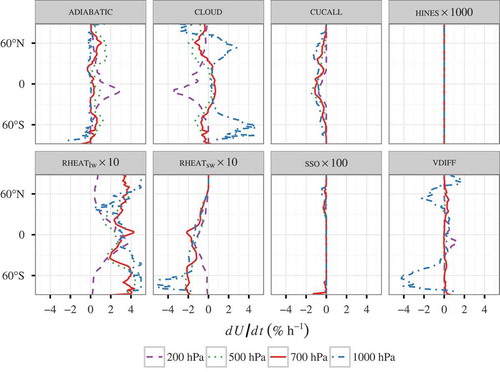
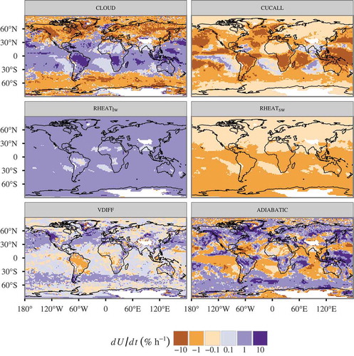
Fig. 2. Monthly mean contributions to the U tendency by the parameterised processes (CLOUD, CUCALL, VDIFF, RHEAT_lw and RHEAT_sw) and ADIABATIC at 700 hPa (absolute percentage values for the relative humidity; note the non-linear scale). HINES and SSO are not shown owing to the negligible size of their contributions.

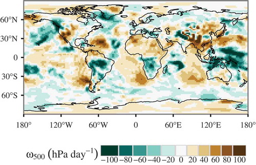
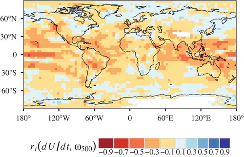
The geographical distribution of the mid-tropospheric (grid-scale) vertical velocity (ω₅₀₀) is shown in Fig. 3. The pattern of vertical motion is similar to CUCALL and ADIABATIC; in the tropics, it is similar (but of opposite sign) to CLOUD.

Fig. 3. Monthly mean distribution of the (grid-scale) vertical wind at the 500 hPa level (ω₅₀₀).

Only near the surface is ADIABATIC small compared to the larger effect of turbulence (VDIFF). VDIFF increases U in the tropics and decreases it in the mid-latitudes at 1000 hPa. This decrease, mainly over the oceans where the 1000 hPa surface exists, is probably attributable to mixing of humidity away from the surface into the boundary layer.

To show the influence of q and T tendencies on the U tendency, we plot the two terms of eq. (1) in Fig. 4 separately for the dominant processes and for DRY, defined as the sum of VDIFF, HINES, RHEAT_lw, RHEAT_sw and SSO (the diabatic processes that do not include phase changes).

Fig. 4. Monthly mean contributions to the U tendency due to the q tendency (left column) and the T tendency (right column) by the main processes in January at 700 hPa. Top row: stratiform cloud processes; second row: cumulus convection; third row: sum of all other diabatic processes; bottom row: adiabatic processes.

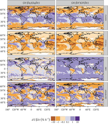
In general, contributions of both moisture and temperature tendencies to the U tendency tend to act in the same direction for all processes in most regions; processes that moisten the atmosphere tend to be accompanied by a cooling, and those that dry the atmosphere by a warming. This is the case for vertical motions (ADIABATIC, CUCALL) and for phase changes (CLOUD, CUCALL). An exception is radiative cooling, which does not affect specific humidity (seen in DRY).

CLOUD increases U in the tropics (30 °S to 30 °N) and decreases it in the middle and high latitudes through both the q and T tendency terms (see next section for a more detailed analysis). The exception to this pattern occurs at 1000 hPa, where U is increased by CLOUD also at middle and high latitudes, and at 200 hPa, where CLOUD decreases U at all latitudes, but more so in the tropics than in the middle to high latitudes, as shown in Fig. 1. The latter effect is due to the height of the tropopause, which is lower in higher latitudes than in the tropics; thus, in middle and high latitudes no condensation/deposition occurs at 200 hPa, near the tropopause, but it does occur in the tropics, where the tropopause is well above 200 hPa. The strong decrease in relative humidity in the tropics is due to depositional growth of ice clouds, whose water vapour supply is adiabatic transport (Fig. 1; see also discussion in the next section). At all levels (but shown here only for the 700 hPa level in Fig. 4), the effect of the q tendency on U is stronger than that of the T tendency.

CUCALL mainly has an effect in the tropics, where most deep convection occurs. It decreases U through both the q and T tendencies, mainly through the effect of compensating subsidence in the deep convection regions, which at the same time dries and warms the atmosphere.

At all heights except near the surface, DRY is mainly influenced by RHEAT_lw, which cools the atmosphere by emission of terrestrial radiation, increasing U. This effect is weakened by absorbed solar radiation, which is represented by RHEAT_sw and acts mainly in the southern hemisphere because the simulation spans the month of January. At 1000 hPa, VDIFF is of importance as well (see above), and increases U in the tropics and decreases U in the mid-latitudes.

ADIABATIC represents adiabatic warming or cooling through large-scale vertical motion as well as horizontal convergence or divergence of water vapour and temperature. In regions of updraught, adiabatic cooling coincides with transport of moist air from the ground to higher altitudes, thus increasing relative humidity. Poleward sensible heat transport, which in isolation would lead to a negative U tendency due to positive T tendency at high latitudes, is offset by positive U tendency due to moisture advection from lower latitudes. Overall, the latter dominates the U tendency, resulting in a positive U tendency due to the poleward transport of warm, moist air.

The U tendency due to the CLOUD subprocesses (CLOUD_cnd, CLOUD_tbl, CLOUD_evr, CLOUD_evl, CLOUD_dep, CLOUD_tbi, CLOUD_sbs, CLOUD_sbi, CLOUD_sbis, CLOUD_mls, CLOUD_mli, CLOUD_mlis, CLOUD_frh, CLOUD_sacl), calculated from monthly mean fields, is shown at 700 hPa in Fig. 5 and zonally averaged at 1000, 700, 500 and 200 hPa in Fig. 6. The sum of these is plotted as ‘CLOUD total’ in Fig. 5, which is equivalent to CLOUD in Figs 1–4. CLOUD_tbi and CLOUD_tbl do not influence U as parameterised in ECHAM; they, along with CLOUD_frl, whose contribution is negligible, have been omitted. The dominant components of CLOUD are CLOUD_dep, CLOUD_sbi and CLOUD_evl, with locally important contributions in the lower troposphere by CLOUD_cnd and CLOUD_sbs in the mid-latitudes and CLOUD_evr in the lower tropical troposphere.

Fig. 5. Monthly mean contributions to the U tendency via q and T tendencies by the subprocesses of CLOUD at 700 hPa. CLOUD_tbl and CLOUD_tbi do not have any effect on U in the model.

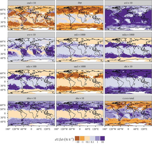
Fig. 6. Monthly and zonal mean contributions to the U tendency by the subprocesses of CLOUD. Note that the tendencies due to various processes have been scaled for better intercomparability. The 1000 hPa line is restricted to ±6% h⁻¹ to fit on the common scale. CLOUD_tbl, CLOUD_tbi and CLOUD_frl, whose contributions to the tendency are negligible, are not shown.

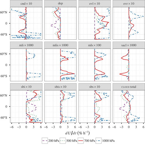
CLOUD_dep (the deposition of water vapour or sublimation of cloud ice) decreases U, indicating that deposition of water vapour, rather than sublimation of ice, is dominant. In the high and middle latitudes, deposition is strongest in the lower troposphere, while in the tropics it is strongest in the upper troposphere, as is to be expected from the tropospheric temperature structure.

CLOUD_evl (the instantaneous evaporation of cloud liquid water which is transported into the cloud-free part of the grid cell) increases U and acts at the height where most liquid-phase clouds appear (Fig. 6). As a large part of cloud formation in the middle and high latitudes takes place in the ice phase and mixed phase, this process mainly acts in the lower latitudes.

U is increased strongly by CLOUD_sbi in the middle and high latitudes. CLOUD_sbi is the instantaneous sublimation of cloud ice which is transported into the cloud-free part of the grid cell. It shows a complementary structure to CLOUD_evl, acting where ice clouds are prevalent. Its pattern is also similar to that of CLOUD_dep, with opposite sign and reduced magnitude. As a result, the total U tendency due to CLOUD is negative in the middle and high latitudes.

In the lower troposphere (700 hPa), CLOUD_cnd has a strong influence on the tendency of U. The net decrease in U is due to the fact that the condensation of water vapour is, on average, greater than the evaporation of cloud liquid water, with the remainder of the condensed water removed in the form of precipitation.

4. Representativeness of monthly mean diagnostics

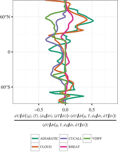
From the CMIP5 models, only monthly mean output for the tendency diagnostics is available. Is this sufficient to analyse the changes in relative humidity? To assess this, we compare the tendencies of relative humidity computed from instantaneous tendencies of q and T (4464 time-steps, shown in temporal average in Fig. 1) and from monthly averaged tendencies of q and T. Owing to the nonlinearity of U in T, a difference is to be expected; the question is whether eq. (1) can be approximately linearised as

(3)

where the operator denotes temporal averaging. Figure 7 shows the relative difference between the U tendency calculated for every time-step and then averaged, in accordance with the left-hand side of eq. (3), and the U tendency calculated from monthly mean q, T, dq/dt and dT/dt fields according to the right-hand side of eq. (3). The differences are within ±25% in the zonal mean except for CLOUD and ADIABATIC in the middle latitudes, where the differences reach 40% and 50%, respectively. We conclude that time averaging can be approximately linearised, and that we can use the monthly mean q and T fields and their monthly mean tendencies to infer the monthly mean tendency of U. This is particularly useful since monthly mean q and T tendencies due to parameterised processes have been archived by many GCMs in CMIP5.

Fig. 7. Relative difference between U tendencies calculated from instantaneous temperature and humidity fields and U tendencies calculated from monthly mean zonal mean fields at 700 hPa.

5. Usefulness of the mid-tropospheric vertical wind in predicting relative humidity tendencies

In this section, we investigate the extent to which variability in the processes analysed in the previous section can be related to variability in the mid-tropospheric vertical wind ω₅₀₀. We do so by analysing the (Pearson product-moment) correlation coefficient r_t between the time series of ω₅₀₀ and the tendencies in relative humidity due to the various processes from instantaneous model output.

In a second step, we determine whether the temporal correlation coefficient based on monthly means in a longer model run can be used as a proxy for temporal correlation based on temporally highly resolved (ideally instantaneous, as done here) data. This step addresses the question of how to proceed when high-frequency data are not available, as is the case in the monthly mean CMIP5 archive. To determine the suitability of monthly mean quantities, we perform a 20 yr simulation (i.e. 240 monthly mean output steps) with monthly mean diagnostics for the relevant quantities and analyse the correlation between the monthly mean tendencies in U and the monthly mean ω₅₀₀.

In many cases, the same parameterisation includes both cloud-forming and cloud-dissolving processes (e.g. CLOUD_cnd includes condensation and evaporation of liquid water, depending on saturation). To distinguish between the cloud-forming and cloud-dissolving processes, we calculate correlation coefficients separately for cases where the parameterisation results in dU/dt > 0 and cases where the parameterisation results in dU/dt < 0.

Figs 8 and 9 show the correlation coefficient between relative humidity tendencies due to various processes at 700 hPa and ω₅₀₀ for the cases in which these processes decrease U and increase U, and for the entire time series regardless of the sign of the contribution to the U tendency by these processes. In the case of Fig. 8, the correlation is calculated based on instantaneous output over the course of 1 month; in the case of Fig. 9, the correlation is calculated based on monthly mean output over the course of 20 yr. The degree to which the results in Figs 8 and 9 are similar indicates the extent to which monthly mean ω₅₀₀ is a good proxy for the instantaneous cloud-forming and cloud-dissolving processes.

Fig. 8. Temporal correlation coefficient between instantaneous ω₅₀₀ and contributions to the instantaneous U tendency by CUCALL, CLOUD_evl, CLOUD_sbi, CLOUD_dep and ADIABATIC at 700 hPa. The correlation coefficient is only plotted when the underlying time series contains n > 100 data points, roughly corresponding to an uncertainty σ (r_t) < 0.1.

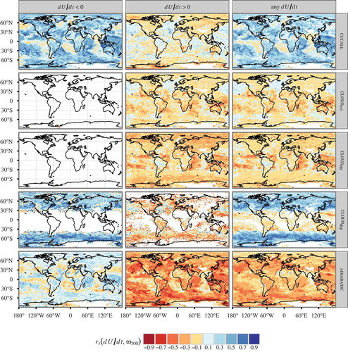
Fig. 9. Temporal correlation coefficient between monthly mean ω₅₀₀ and contributions to the monthly mean U tendency by CUCALL, CLOUD_evl, CLOUD_sbi, CLOUD_dep and ADIABATIC at 700 hPa. The correlation coefficient is only plotted when the underlying time series contains n > 100 data points, roughly corresponding to an uncertainty σ (r_t) < 0.1.

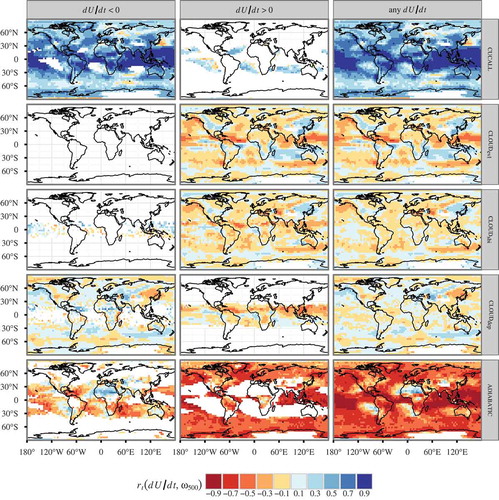
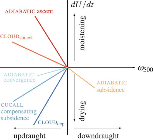
We have chosen to discuss the processes that contribute most strongly to the overall dU/dt, namely CUCALL, CLOUD_evl, CLOUD_sbi, CLOUD_dep and ADIABATIC. Fig 10 summarises the relationships between ω₅₀₀ and dU/dt for these processes schematically.

Fig. 10. Schematic of the position in dU/dt–ω₅₀₀ phase space of the various processes; the colour indicates the strength of the correlation on the same scale as in Fig. 8.

As expected, the general qualitative behaviour when analysed over large regions is usually similar between the high- and low-frequency correlations. However, substantial differences are found quantitatively and in some cases also qualitatively.

5.1. CUCALL

CUCALL is shown in the first row of Fig. 8. In cases where the CUCALL contribution to the U tendency is positive, the correlation with ω₅₀₀ is small. In cases where the CUCALL contribution to the U tendency is negative, the correlation coefficient is large and positive, especially in the tropics in regions of large-scale ascent. In the subsidence regions, convective mass fluxes are small, and the relationship between ω₅₀₀ and dU/dt due to CUCALL is therefore weak; in these regions, small correlation coefficients of either sign prevail.

The reason for the predominant strongly negative correlation coefficients is that the large-scale q and T fields in the middle troposphere are affected by CUCALL primarily through the compensating subsidence (Möbis and Stevens, 2012). In the tropics, the convective mass flux, and therefore the compensating subsidence, correlates with the large-scale ω₅₀₀. Because the thermodynamic structure of the tropical atmosphere is moist adiabatic, the compensating subsidence causes adiabatic heating as well as vertical advection of low specific humidity, both of which lead to drying. In the tropics, the correlation coefficient between the U tendency and ω₅₀₀ tests how good a proxy the large-scale vertical motion is for cumulus convection. In the extratropics, we expect the link between large-scale vertical motion and cumulus convection to be weaker; the correlation coefficient is correspondingly smaller. Finally, for CUCALL to produce a positive relative humidity tendency (i.e. moistening) through compensating subsidence, an unusual thermodynamic profile is required; this case occurs rarely, and the correlation with ω₅₀₀ in this case is small.

The temporal correlation in low-frequency output is high and qualitatively resembles the correlation in the high-frequency output; in many regions, the low-frequency correlation is greater than the high-frequency correlation owing to the averaging out of noise in the monthly means. Regional features that are evident in the high-frequency output, such as the negative correlation in the subsidence regions, disappear in the monthly mean correlations because the underlying process occurs too infrequently to affect the monthly means strongly.

5.2. CLOUD_evl, CLOUD_sbi and CLOUD_dep

The second to fourth rows of Figs 8 and 9 show the correlation coefficients between ω₅₀₀ and the contribution to dU/dt by the major subprocesses of CLOUD, namely CLOUD_evl, CLOUD_sbi and CLOUD_dep.

CLOUD_evl and CLOUD_sbi, the instantaneous evaporation or sublimation of cloud condensate transported into the cloud-free part of a grid cell, can only increase U. [Nevertheless, owing to numerical artefacts, the dU/dt diagnostic is occasionally negative; these cases are rare enough that the requirement of n > 100 data points removes them from Fig. 8. In the monthly means, owing to the inexact equality of eq. (3), negative tendencies are more frequent and can be seen in Fig. 9.] The U tendencies due to CLOUD_evl and CLOUD_sbi are negatively correlated with ω₅₀₀ at 700 hPa, with generally small correlation coefficients, as large-scale ascent is associated with large-scale cloud formation; more abundant large-scale cloud leads to more frequent evaporation or sublimation in the cloud-free parts of the grid box. For CLOUD_evl, this correlation is strongest in the tropical ascent regions (where the 700 hPa temperature is sufficiently high), while for CLOUD_sbi the correlation is strongest in the extratropics. Comparing the low-frequency correlation to the high-frequency correlation, we see that, even qualitatively, large differences exist, including regional changes of sign. In large part, these differences stem from correlations due to the seasonal cycle in both ω₅₀₀ and the tendencies; in Fig. 11, when we have removed the seasonal cycles by subtracting the 20 yr mean for each calendar month from both variables, we recover a spatial pattern qualitatively consistent with the high-frequency correlations. As is the case for CUCALL and ADIABATIC, the magnitude of the low-frequency correlation (once deseasonalisation has been performed) is greater than the magnitude of the high-frequency correlation, presumably because high-frequency noise is averaged out in the monthly means.

Fig. 11. Temporal correlation coefficient between monthly mean ω₅₀₀ and monthly mean U tendency due to CLOUD_evl at 700 hPa; the seasonal cycle in both ω₅₀₀ and CLOUD_evl has been removed by subtracting the 20 yr mean quantity for each calendar month.

The correlation coefficient between ω₅₀₀ and dU/dt due to CLOUD_dep is large and positive (frequently, r_t > 0.5) in cases of drying and negative in cases of moistening. Overall, the drying dominates at 700 hPa. The negative correlation coefficients in the dU/dt< 0 case are large because ω₅₀₀ is a good predictor for drying by deposition in the case of updraught. ω₅₀₀ is a reasonable predictor for moistening by sublimation in the case of downdraught; in this case, however, the cloud amount decreases with increasing subsidence, and therefore the (grid-box mean) tendency is negatively correlated with ω₅₀₀. At 700 hPa, temperatures are usually above freezing in the tropics, so that the correlation between ω₅₀₀ and CLOUD_dep can be seen most clearly in the mid-latitude storm tracks. The positive correlation stems from the correlation between ω₅₀₀ and cloud microphysical processes in storm-track depressions, which is averaged out on longer than synoptic timescales; therefore, the monthly mean ω₅₀₀ is not well correlated with the monthly mean CLOUD_dep diagnostics.

5.3. ADIABATIC

The correlation between ω₅₀₀ and dU/dt due to ADIABATIC is negative at 700 hPa. The net negative correlation is the result of a strong negative correlation in the moistening (dU/dt> 0) case and a weak positive correlation in the drying (dU/dt< 0) case. The negative correlation in the moistening case is due to the adiabatic cooling and the vertical advection of high specific humidity in large-scale ascent. In the drying case, there is a weakly negative correlation between ω₅₀₀ and dU/dt in the subsidence regions, which can be explained by the adiabatic heating and vertical advection of low specific humidity in subsidence. Outside the subsidence regions, the correlation between dU/dt and ω₅₀₀ is weakly positive; a process that could explain this relationship is horizontal advection of relatively dry air into regions of large-scale ascent.

In the low-frequency output, the ADIABATIC tendency mainly reflects the large-scale pattern of ascent and descent. As a result, the subsidence regions are clearly visible in an overall field of negative correlation caused by increasing moistening with increasing updraught. As in the case of CUCALL, the correlation coefficients in the low-frequency output are greater than in the high-frequency output owing to the averaging out of high-frequency noise.

6. Summary and conclusions

Instantaneous tendency diagnostics of the change in specific humidity q and temperature T and, consequently, of relative humidity U during a 1 month simulation (January) with the ECHAM6 GCM were analysed. The dominant processes for cloud formation and dissolution are adiabatic processes, cloud microphysical processes (including stratiform condensation and deposition) and, a little less dominantly, convection. In the lower and middle troposphere, the influence of cloud microphysics is dominated by evaporation and sublimation in response to horizontal subgrid-scale mixing, and by deposition/sublimation of cloud ice, i.e. phase changes between water vapour and cloud water and ice. In the lower troposphere, large-scale condensation is relevant in the mid-latitudes, while evaporation of falling rain is relevant in the tropics.

The correlations of the considered diagnostics to the mid-tropospheric vertical velocity ω₅₀₀ were analysed. The processes listed above as dominant for relative humidity changes are well correlated with ω₅₀₀; Fig. 10 summarises the strength of the correlation between processes as well as the quadrant in dU/dt–ω₅₀₀ space that contributes most strongly to the correlation. For model analysis, this result supports the common practice of using ω₅₀₀ to define cloud regimes to the extent that cloud regimes are determined by the dominant cloud-forming and cloud-dissolving processes.

Often only monthly mean model diagnostics are available. To test the feasibility of our analysis when using monthly mean data, we have compared results based on instantaneous data with results based on monthly mean data. We found that for the contribution of the individual processes to the U tendency, there is approximate linearity in the temporal average. Comparing the temporal correlation of instantaneous process tendency diagnostics and instantaneous ω₅₀₀ with the correlation between monthly mean diagnostics and monthly mean ω₅₀₀, we find that in the storm tracks, cloud microphysical processes are poorly constrained by monthly mean ω₅₀₀. Regional features related to convection are also averaged out when considering only monthly means, while the overall correlation between ω₅₀₀ and CUCALL and ADIABATIC is strengthened owing to the averaging out of high-frequency noise. In most other cases, we therefore find a broad qualitative agreement between the high-frequency and low-frequency correlations.

Acknowledgements

This study was funded by the European Research Council (ERC) through the Starting Grant ‘QUAERERE’ (grant agreement no. 306284). We would like to thank the Max Planck Institute for Meteorology for developing and making available the ECHAM6 model, and the German Climate Computing Centre (DKRZ) for providing computing resources. We acknowledge support from the German Research Foundation (DFG) and Universität Leipzig through the DFG open access publication fund. We thank three anonymous reviewers for constructive suggestions.

Disclosure statement

No potential conflict of interest was reported by the authors.

Additional information

Funding

This work was supported by the European Research Council (ERC) [306284].

References

- Bjerknes, J. 1919. On the structure of moving cyclones. Mon. Wea. Rev. 47, 95–99. DOI: 10.1175/1520-0493(1919)47<95:OTSOMC>2.0.CO;2.
- Bony, S., Bellon, G., Klocke, D., Sherwood, S., Fermepin, S. and co-authors 2013. Robust direct effect of carbon dioxide on tropical circulation and regional precipitation. Nat. Geosci. 6, 447–451. DOI: 10.1038/ngeo1799.
- Bony, S., Dufresne, J.-L., Le Treut, H., Morcrette, J.-J. and Senior, C. 2004. On dynamic and thermodynamic components of cloud changes. Clim. Dyn. 22, 71–86. DOI: 10.1007/s00382-003-0369-6.
- Brinkop, S. and Roeckner, E. 1995. Sensitivity of a general-circulation model to parameterizations of cloud–turbulence interactions in the atmospheric boundary layer. Tellus A 47(2), 197–220. DOI: 10.1034/j.1600-0870.1995.t01-1-00004.x.
- Davies, L., Jakob, C., May, P., Kumar, V. V. and Xie, S. 2013. Relationships between the large-scale atmosphere and the small-scale convective state for Darwin, Australia. J. Geophys. Res. Atmos. 118, 11534–11545. DOI: 10.1002/jgrd.50645.
- Giorgetta, M. A., Roeckner, E., Mauritsen, T., Stevens, B., Bader, J. and co-authors. 2013: The Atmospheric General Circulation Model ECHAM6 – Model Description. Technical Report 135, Max Planck Institute for Meteorology, Hamburg, Germany. Online at: http://www.mpimet.mpg.de/fileadmin/publikationen/Reports/WEB_BzE_135.pdf
- Govekar, P. D., Jakob, C. and Catto, J. 2014. The relationship between clouds and dynamics in southern hemisphere extratropical cyclones in the real world and a climate model. J. Geophys. Res. Atmos. 119, 6609–6628. DOI: 10.1002/2013JD020699.
- Gryspeerdt, E. and Stier, P. 2012. Regime-based analysis of aerosol-cloud interactions. Geophys. Res. Lett. 39(L21), 802. DOI: 10.1029/2012GL053221.
- Gryspeerdt, E., Stier, P. and Partridge, D. G. 2014. Satellite observations of cloud regime development: the role of aerosol processes. Atmos. Chem. Phys. 14, 1141–1158. DOI: 10.5194/acp-14-1141-2014.
- Howard, L. 1803. Essay on the Modifications of Clouds. John Churchill and Sons, London.
- Iacono, M. J., Delamere, J. S., Mlawer, E. J., Shephard, M. W., Clough, S. A. and co-authors 2008. Radiative forcing by long-lived greenhouse gases: calculations with the AER radiative transfer models. J. Geophys. Res. 113(D13), 103. DOI: 10.1029/2008JD009944.
- Jakob, C. and Tselioudis, G. 2003. Objective identification of cloud regimes in the Tropical Western Pacific. Geophys. Res. Lett. 30, 2082. DOI: 10.1029/2003GL018367.
- Klein, S. and Hartmann, D. 1993. The seasonal cycle of low stratiform clouds. J. Climate 6, 1587–1606. DOI: 10.1175/1520-0442(1993)006<1587:TSCOLS>2.0.CO;2.
- Lauer, A., Hamilton, K., Wang, Y., Phillips, V. T. J. and Bennartz, R. 2010. The impact of global warming on marine boundary layer clouds over the eastern Pacific–a regional model study. J. Climate 23(21), 5844–5863. DOI: 10.1175/2010JCLI3666.1.
- Lohmann, U. and Roeckner, E. 1996. Design and performance of a new cloud microphysics scheme developed for the ECHAM general circulation model. Clim. Dynam. 12(8), 557–572. DOI: 10.1007/BF00207939.
- Medeiros, B. and Stevens, B. 2011. Revealing differences in GCM representations of low clouds. Clim. Dyn. 36, 385–399. DOI: 10.1007/s00382-009-0694-5.
- Miller, R. L. 1997. Tropical thermostats and low cloud cover. J. Climate 10, 409–440. DOI: 10.1175/1520-0442(1997)010<0409:TTALCC>2.0.CO;2.
- Möbis, B. and Stevens, B. 2012. Factors controlling the position of the intertropical convergence zone on an aquaplanet. J. Adv. Model. Earth Syst. 4, M00A04. DOI: 10.1029/2012MS000199.
- Morcrette, C. J. and Petch, J. C. 2010. Analysis of prognostic cloud scheme increments in a climate model. Q.J.R. Meteorol. Soc. 136, 2061–2073. DOI: 10.1002/qj.720.
- Mülmenstädt, J., Lubin, D., Russell, L. M. and Vogelmann, A. M. 2012. Cloud properties over the North Slope of Alaska: identifying the prevailing meteorological regimes. J. Climate 25(23), 8238–8258. DOI: 10.1175/JCLI-D-11-00636.1.
- Nam, C. C. W. and Quaas, J. 2013. Geographically versus dynamically defined boundary layer cloud regimes and their use to evaluate general circulation model cloud parameterizations. Geophys. Res. Lett. 40, 4951–4956. DOI: 10.1002/grl.50945.
- Ogura, T., Emori, S., Webb, M. J., Tsushima, Y., Yokohata, T. and co-authors 2008. Towards understanding cloud response in atmospheric GCMs: the use of tendency diagnostics. J. Meteorol. Soc. Japan 86, 69–79. DOI: 10.2151/jmsj.86.69.
- Oreopoulos, L., Cho, N., Lee, D., Kato, S. and Huffman, G. J. 2014. An examination of the nature of global MODIS cloud regimes. J. Geophys. Res. Atmos. 119, 8362–8383. DOI: 10.1002/2013JD021409.
- Stevens, B. 2005. Atmospheric moist convection. Annu. Rev. Earth Planet. Sci. 33, 605–643. DOI: 10.1146/annurev.earth.33.092203.122658.
- Stevens, B. and Feingold, G. 2009. Untangling aerosol effects on clouds and precipitation in a buffered system. Nature 461, 607–613. DOI: 10.1038/nature08281.
- Stevens, B., Giorgetta, M., Esch, M., Mauritsen, T., Crueger, T. and co-authors. 2013. Atmospheric component of the MPI-M Earth System Model: ECHAM6. J. Adv. Model. Earth Syst. 5, 146–172. DOI: 10.1002/jame.20015.
- Su, W., Loeb, N. G., Xu, K., Schuster, G. L. and Eitzen, Z. A. 2010. An estimate of aerosol indirect effect from satellite measurements with concurrent meteorological analysis. J. Geophys. Res. 115(D18), 219. DOI: 10.1029/2010JD013948.
- Taylor, K. E., Stouffer, R. J. and Meehl, G. A. 2012. An overview of CMIP5 and the experiment design. Bull. Amer. Meteor. Soc. 93, 485–498. DOI: 10.1175/BAMS-D-11-00094.1.
- Tiedtke, M. 1989. A comprehensive mass flux scheme for cumulus parameterization in large-scale models. Mon. Weather Rev. 117(8), 1779–1800. DOI: 10.1175/1520-0493(1989)117<1779:ACMFSF>2.0.CO;2.
- Tselioudis, G., Rossow, W., Zhang, Y. and Konsta, D. 2013. Global weather states and their properties from passive and active satellite cloud retrievals. J. Climate 26, 7734–7746. DOI: 10.1175/JCLI-D-13-00024.1.
- Williams, K. D. and Tselioudis, G. 2007. GCM intercomparison of global cloud regimes: present-day evaluation and climate change response. Clim. Dyn. 29, 231–250. DOI: 10.1007/s00382-007-0232-2.
- WMO. 1975: International Cloud Atlas, Volume I – Manual on the Observation of Clouds and Other Meteors. Technical report, World Meteorological Organization. Online at: http://library.wmo.int/pmb_ged/wmo_407_en-v1.pdf
- Wood, R. and Bretherton, C. S. 2006. On the relationship between stratiform low cloud cover and lower-tropospheric stability. J. Climate 19, 6425–6432. DOI: 10.1175/JCLI3988.1.