Abstract
Evidence from paleo-proxy records suggests that the Atlantic Meridional Overturning Circulation (AMOC) can be in both an AMOC on state, the AMOC as we observe it today, and an AMOC off state, where the AMOC becomes extremely weak or even collapses. The freshwater transport due to the AMOC () at 34°S in the Atlantic has often been used as an indicator for bi-stability, with a positive
suggesting a monostable AMOC and a negative
suggesting a bi-stable AMOC. Often studies have shown that the sign of the divergence of the
might be a good indicator of AMOC bi-stability. In this study we investigate how model bias affects the sign of
across all latitudes in the Atlantic basin, through a detailed analysis of the Coupled Model Inter-Comparison Project 5 (CMIP5) model ensemble.
, in the CMIP5 models is generally too positive in the southern Atlantic due to a salinity bias, while in the subtropical North Atlantic the values of
are influenced by a combination of velocity and salinity biases. We compare these results to observations, reanalysis products and Hadley Centre Global Environmental Model version 3 global configuration version 2, a current generation coupled model which exhibits a stable AMOC off state, and discuss the differences that can lead to the possibility of a bi-stable AMOC as opposed to a monostable AMOC.
1. Introduction
The Atlantic Meridional Overturning Circulation (AMOC) forms an important part of the Atlantic climate system, transporting heat northward resulting in warmer temperatures in the regions surrounding the subpolar North Atlantic than other regions at a similar latitude. If the AMOC was to collapse it would have severe impacts on the climate in this region, causing reductions in surface air temperatures of up to 10°C in the North Atlantic according to modelling studies (Manabe and Stouffer, Citation1988; Vellinga and Wood, Citation2002; Jackson et al., Citation2015). Past evidence of temperature changes of these magnitudes has been observed in paleo-proxy records (Dansgaard et al., Citation1993; Blunier and Brook, Citation2001; de Abreu et al., Citation2003), and was originally linked to the possibility of a bi-stable AMOC by Broecker et al. (Citation1990). Projecting present day climate change into the future through the representative concentration pathways, models from the Coupled Model Inter-Comparison Project 5 (CMIP5) show evidence for a weakening of the AMOC circulation of 11–34% by 2100, while a complete collapse is deemed unlikely (Collins et al., Citation2013). However, several studies suggest that models might be too stable, affecting the likelihood of simulating future abrupt climate change (Valdes, Citation2011; Drijfhout et al., Citation2011; Hansen et al., Citation2016). Projections of the AMOC decline under future climate change have shown a greater AMOC decrease in CMIP5 models than in CMIP3, suggesting that improvements to climate models may have resulted in an AMOC that is more sensitive to changes in forcing (Reintges et al., Citation2016).
The possibility for an AMOC switching between an AMOC on state and AMOC off state (a collapsed or weak AMOC) has been a subject of modelling studies for many years, beginning with simple box model studies (Stommel, Citation1961; Marotzke, Citation1990; Rahmstorf, Citation1996) and continuing up to complex climate model studies (Manabe and Stouffer, Citation1988; Stouffer et al., Citation2006; Mecking et al., Citation2016). The freshwater transport by the AMOC has been proposed as an indicator of AMOC bi-stability (Rahmstorf, Citation1996; de Vries and Weber, Citation2005) and is referred to as (
in some studies). When used as an indicator for AMOC bi-stability,
is typically measured at the southernmost boundary of the Atlantic Ocean at 34°S. A positive value of
at 34°S indicates that the AMOC is importing freshwater into the Atlantic, while for a negative
at 34°S the AMOC imports salt into the Atlantic. When the AMOCcollapses
initially tends towards zero. Therefore, in the case of an AMOC collapse an initial positive (negative) value of
will cause an anomalous import of salt (freshwater) into the Atlantic destabilising (stabilising) the AMOC off state. Consequently, a positive value of
suggests a monostable AMOC regime, while a negative
at 34°S suggests a bi-stable AMOC. Observational estimates of
near the southern boundary suggest that
is negative and therefore the AMOC in the current climate system is in a bi-stable regime (Bryden et al., Citation2011; Garzoli et al., Citation2013).
becomes an imperfect indicator of the AMOC response to salinity perturbations since the subtropical gyre in the South Atlantic adjusts in conjunction with the AMOC. In that case, the stabilising effects of the gyre salt transport at 34°S have to be taken into account Sijp (Citation2012). Also, in several cases where the AMOC can sustain an AMOC off state a reverse thermohaline circulation (RTHC) develops (Yin and Stouffer, Citation2007; Sijp, Citation2012). The development of RTHC increases the freshwater transport into the Atlantic by the AMOC helping to further stabilise the AMOC off state. This
value, however, is no longer associated with the behaviour of the AMOC on state. In the AMOC on state
is a measure for the advective salt feedback between northward salt transport and northern sinking, but this no longer occurs in the RTHC. To measure the stability of the RTHC, another indicator is needed. Several studies have suggested that the divergence of the
across the Atlantic is a better indicator for bi-stability (Huisman et al., Citation2010; Liu and Liu, Citation2013). Yin and Stouffer (Citation2007) proposed to use the divergence of
across the subtropical North Atlantic as an indicator, which was also supported by Mecking et al. (Citation2016).
Table 1. Table containing a list of all the markers used to identify the models, model name, the institute that conducted the experiments, the values of AMOC at 26.5°N, at 34°S and
at 26.5°N. The values with a grey shading for
fall within the range of observational estimates. The stars behind the model names indicate the models for which freshwater fluxes were available in the CMIP5 model database.
This study investigates the proposed bi-stability indicators in 43 CMIP5 models and how they depend on model bias, in particular the salinity bias. Weaver et al. (Citation2012) have previously examined in 30 CMIP5 and EMIC models however, that study only focused on the values at the southern boundary of the Atlantic. Here we investigate
over the entire Atlantic and how it is affected by model bias over 43 CMIP5 models, two renanalysis products and a current generation coupled climate model. Liu et al. (Citation2014) and Liu et al. (Citation2017) suggested that model bias could have an impact on the
, although the quantitative impact was not investigated in detail. This paper begins with a brief description of the models and the data used in this study, as well as the mathematical framework for the calculation of
(Section 2). In Section 3 the values of
across the CMIP5 models and reanalysis are analysed and in the following section (Section 4) the role of the atmosphere in generating salinity bias is discussed. Finally the paper is concluded with a discussion on the implications for AMOC bi-stability (Section 5).
2. Data and methods
2.1. Models and data
For this study the historical simulations from 43 models in the CMIP5 (Taylor et al., Citation2012) have been used (See Table ). Several of the CMIP5 models have more than one ensemble member available but for this study only the first ensemble member was used. The analysis was performed on the original model grid on which the data were presented with the exception of the models’ vertical grid in inmcm4, MIROC-ESM, MIROC-ESM-CHEM and MIROC5. The data for these models were not stored on z-levels, which are necessary for our analysis. Hence they were interpolated onto regular z-levels using a conservative interpolation scheme. In all cases, the computations were conducted using monthly mean data and then averaged over the period of 1960–1989.
Without many full depth observational estimates of ocean currents throughout the Atlantic it is difficult to accurately assess how well the models are performing with their values of across the Atlantic. In this study, we are limited to a handful of latitudes where observation-based values of
exist (Fig. a). Therefore it is useful to turn to reanalysis products which assimilate observations into the models. For that we turn to version 2.2.4 of the Simple Ocean Data Assimilation (SODA) ocean reanalysis product (Carton and Giese, Citation2008), a reanalysis product that goes quite far back in time starting at 1870 and GloSea5, which has been shown to compare well with the AMOC strength and variability at 26.5N (Jackson et al., Citation2016). Due to the limited number of years available in GloSea5 data, comparisons were made using a mean from 1995–2012 while 1960–1989 was used for SODA.
The current generation coupled climate model Hadley Centre Global Environmental Model version 3 global configuration version 2 (HadGEM3-GC2) (Williams et al., Citation2015) was able to sustain an AMOC off state for 450 years (Mecking et al., Citation2016). A historical simulation with the same set-up as the CMIP5 models will be used to compare to the CMIP5 models. This model configuration is also used in the operational seasonal and decadal forecast systems of the Met Office (GloSea5 and DEPRESYS3). The ocean model is the Global Ocean 5.0 (Megann et al., Citation2014) version of the v3.4 NEMO model (Madec, Citation2008) and uses the ORCA025 tripolar grid configuration. It has 75 vertical levels, and a nominal horizontal resolution of 0.25 degrees (compared to the typical 1 degree resolution of the CMIP5 models). The historical simulation ran from 1850 using initial conditions from a GC2 pre-industrial control run and again the mean from 1960-1989 is used.
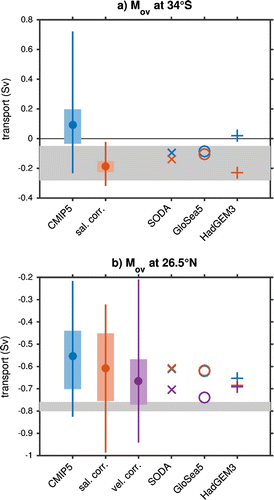
Figure 1. The range of the values of a) at 34°S and b)
at 26.5°N for the historical mean (blue), salinity bias corrected (orange) and for 26.5°N velocity bias corrected (purple). For the CMIP5 models the range of model values (vertical line), multi-model mean (dot) and the range of the models falling in the middle half (shaded box). The shading indicates the observational estimates of
at 34°S as estimated by Garzoli et al. (Citation2013) (note that other observational estimates fall within that range) and
at 26.5°N as computed by McDonagh et al. (Citation2015).
When comparing the model data to observations, for salinity the EN3 data-set was used (Ingleby and Huddleston, Citation2007) withmonthly data averaged over 1960–1989. For comparisons with observed meridional transports at 26.5°N, data from the RAPID mooring array were used, averaged from April 2004 to March 2014 (Smeed et al., Citation2015). Also, various estimates of freshwater transports are available: (1) Garzoli et al. (Citation2013), which use XBT-derived estimates over the years 2002–2011 at 35°S, ARGO climatology at 30°S as well as CTD data at 30°S from two cruises in 1993 and 2003, (2) values based on the data from the transects near 34°S made in 1992 and 1993 used in McDonagh and King (Citation2005), McDonagh (Personal Communication), (3) Bryden et al. (Citation2011) which uses data from two ship transacts at 24°S in 1983 and 2009, (4) McDonagh et al. (Citation2015) which uses continuous data from the RAPID mooring array and ARGO floats from April 2004 to October 2012 and (5) McDonagh et al. (Citation2010) which uses hydrographic section data at 36°N in 2005.
2.2. Mathematical framework
This study investigates the impacts of model bias on the freshwater transports due to the AMOC. Several of the models in the CMIP5 database did not have the AMOC as part of the output provided and sometimes it was provided as a mass transport as opposed to a volume transport. Therefore, to remain consistent we computed the AMOC streamfunction based on monthly mean meridional currents. The AMOC streamfunction, , is computed as follows,
(1)
where the depth of the ocean is given by and
is the meridional velocity with the section mean removed (i.e.
,
) and the W and E refer to the western and eastern boundaries of the Atlantic Ocean. The freshwater transports due to the AMOC,
, are computed following de Vries and Weber (Citation2005):
(2)
where the baroclinic component of the zonal mean meridional velocity is given as and the zonal mean gives as
, with f being either meridional velocity or salinity. In several studies a value of 35 psu is used for the the reference salinity,
. However, in this study the reference salinity is computed as
, with the impact of this choice being very minimal, less than 1 mSv (Mecking et al., Citation2016). It should be pointed out that the meridional velocity used in the computation of
is the same as the one used in the computation of the AMOC streamfunction
(i.e.
), suggesting that they are strongly connected. Furthermore, the azonal or gyre component of the freshwater transports,
is given as follows,
(3)
where is the departure from the zonal mean for any arbitrary f.
The computations were carried out on the model grid as opposed to moving the data onto a constant latitude. In all models the grid follows approximately constant latitude in the x direction throughout most of the Atlantic, especially in the South Atlantic. In the Arctic, the grids are less close to latitude lines and vary across models since they use different methods to handle the potential singularity at the North Pole. Hence, we limit our calculations to south of 65°N. The latitude values given in this study are based on the average latitude along a line of constant y, with the exception of the at 34°S in which the first line of latitude which is not part of the Southern Ocean, or the line of latitude closest to 34°S, whichever is furthest north, is used.
3. Freshwater transports due to AMOC
3.1.  at 34°S
In the 43 CMIP5 models the values of at 34°S vary from —0.23 Sv (CMCC-CESM) to 0.72 Sv (FGOALS-g2) with a multi-model mean of 0.09 Sv (Table , Fig. a). Observational estimates of
near 34°S all fall within the range of –0.28 to –0.05 Sv (Garzoli et al., Citation2013; Bryden et al., Citation2011, McDonagh (Personal Communication), based on McDonagh and King (Citation2005)). Only 8 out of the 43 CMIP5 models fall within this range, with all the other CMIP5 models having a too positive
(Fig. a). Only 18 of the CMIP5 models have negative values of
, which would suggest from theory a bi-stable AMOC. However, 10 of the 18 values are between 0 Sv and –0.05 Sv, implying that these models are close to the boundary between mono- and bi-stability. For the models that overlap with (Weaver et al. Citation2012, Stability of the AMOC: A model intercomparison, Geophysical Research Letters, under review) the values of
are consistent with the computations in that paper.
at 34°S from both SODA and GloSea5 have a value of –0.09 Sv which falls within the range of observations (Table , Fig. a).
Figure 2. Scatter plots of the strength of the AMOC at 26.5°N and a) at 34°S, b)
at 26.5°N, c) salinity bias corrected
at 34°S and d) salinity bias corrected
at 26.5°N. For panels a) and c) shading indicates range of values of
at 34°S as estimated by Garzoli et al. (Citation2013) with the vertical black line indicating 0 Sv and in panels b) and d) shading indicates the range of values of
at 26.5°N as estimated by McDonagh et al. (Citation2015). In all the panels the horizontal black line indicates the estimated value of AMOC strength at 26.5°N by Smeed et al. (Citation2014). In the title correlation values that are significant at the 99% level are indicated in red. The dashed lines on the figures show the lines of best fit using a least squares estimate, one line minimises the error in the vertical direction and the other in the horizontal direction. The lines of best fit are computed using the CMIP5 models only.
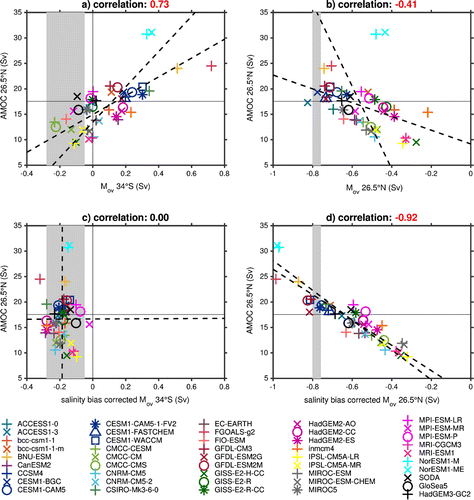
Figure 3. Top panels show the mutli-model mean of (a) and (b)
of the CMIP5 models with the thin lines indicating the range of the model values of both the historical mean (blue) and the salinity bias corrected mean (orange) with the range of the model values indicated by the thinner lighter lines of the same colour. Estimates of
from observations (black): triangle based on McDonagh and King (Citation2005); cross McDonagh et al. (Citation2010); stars Bryden et al. (Citation2011); circles Garzoli et al. (Citation2013) with thevertical line representing the range in estimates; and diamond McDonagh et al. (Citation2015). The bottom panels show (c) the multi-model mean salinity bias from the CMIP5 models for the zonal mean Atlantic salinity bias and (d) the zonal mean Atlantic salinity in the EN3 data.
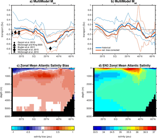
A strong relationship between at 34°S and the AMOC at 26.5°N exists, illustrated by a correlation of 0.73 (significant at 99%) (Fig. a). This suggests that the strength of the AMOC has a significant influence on the value of
. As a result, one would expect that the closer the values of the models’ AMOC are to the observed values of the AMOC (17.55 Sv, Smeed et al., Citation2014), the closer the models’
would be to the observational estimates. However, it turns out that models which have a fairly weak AMOC have values of
closer to the observational estimates, while models with an AMOC strength closer to the observations have almost zero values of
, and models with a too strong AMOC have a positive
. This suggests another reason is causing the large discrepancy between the models’ values of
and observational values. The vertical structure of the zonal mean salinity plays an important role in determining the value of
. Previous studies have found that
is too positive because of salinity biases with models being too fresh near the surface and too saline at depth in the South Atlantic (Yin and Stouffer, Citation2007; Jackson, Citation2013; Mecking et al., Citation2016). To compute the effect of the salinity bias,
is recalculated using the model velocities, but using observed salinities (EN3) interpolated onto each model grid. This is referred to as ‘salinity bias corrected’ in the remainder of the paper. When the salinity bias is corrected, the CMIP5 models’ values are close to the observational range (Fig. a).
is no longer significantly correlated with the AMOC strength (Fig. c), suggesting that at 34°S the strength of the AMOC mainly impacts the magnitude of the salinity bias, while a direct effect on the values of
through the velocity bias is small. It should be noted that the positive correlation implies that the stronger the AMOC, the fresher the South Atlantic thermocline is. Note that the correlation with the AMOC at 26.5°N is almost identical to the correlation with the AMOC at 34°S (local AMOC), both for the uncorrected and salinity bias corrected values of
.
3.2.  at 26.5°N
Before investigating the basin-wide , we take advantage of having a continuous observational estimate available at 26.5°N that spans 8.5 years (McDonagh et al., Citation2015), allowing for a more detailed comparison at this latitude. To make the comparison consistent with the observational estimate we excluded the Gulf of Mexico from the calculations. At 26.5°N the multi-model
of the CMIP5 models is –0.55 Sv, smaller in magnitude (more positive) than the observational estimate of –0.78 Sv (Fig. b). Unlike
at 34°S, only one of the models’ values of
at 26.5°N falls within the observational estimate error bounds (CESM1-BGC), with most of the models having too small of a magnitude but 19 of the 43 models fall within 1 standard deviation of the 10 day means from measurements. Consistent with the CMIP5 models the reanalysis products also have an
at 26.5°N that underestimates the magnitude of the observations. Also, different from
at 34°S the models with the stronger AMOC yield values of
closer to the mean observational estimate (Fig. b). The correlation between AMOC strength at 26.5°N and
at 26.5°N is much weaker than the correlation between AMOC strength at 26.5°N and
at 34°S (Fig. a and b). At first sight this is surprising, since we would expect a greater correlation when comparing the AMOC and
at the same latitude. However, a strong correlation of -0.92 appears when comparing the AMOC to the salinity bias corrected
at 26.5°N. This strong negative correlation is to be expected i.e. the stronger the AMOC at 26.5°N, the weaker the northward freshwater transport/stronger the northwards salt transport. The weaker correlation of –0.41 before correcting the salinity bias implies that the salinity bias at 26.5°N impedes a strong relationship between AMOC and
. As a result, we can infer that due to the salinity bias a spurious relation between AMOC and
is imposed with the AMOC transporting too much freshwater northward, creating a positive bias in
. Without this bias the AMOC transports more salt northward and at 26.5°N the correlation between AMOC and
becomes stronger. Also at 26.5°N the salinity bias is no longer due to the AMOC but due to other processes, for example a net evaporation bias.
Figure 4. The zonal values of for a) SODA and b) GloSea5 for the historical mean (black), salinity bias corrected (grey), CMIP5 multi-model mean (blue) and salinity bias corrected multi-model mean (orange). With black markers indicating the same observational estimates as used in Fig. .
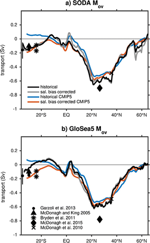
Figure 5. Correlation of the strength of the AMOC at 26.5°N with (blue), the salinity bias corrected
(orange) and the difference between the
and salinity bias corrected
(the correction applied to
) (yellow). Everything outside the shaded region is significant at the 99% level.
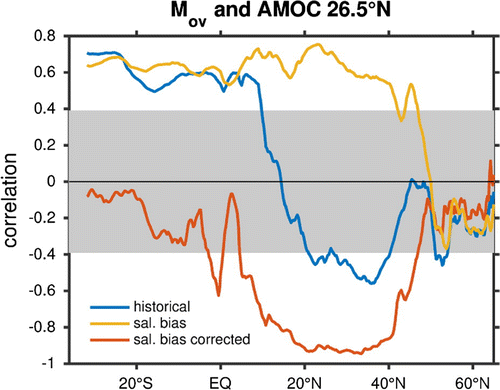
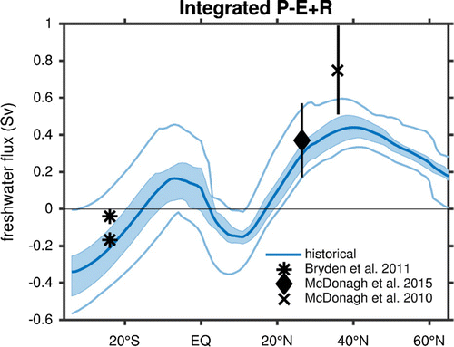
Figure 6. Integrated upward surface freshwater fluxes starting from the Bering Strait to 34°S for the CMIP5 multi-model mean (blue line), the range of all the CMIP5 models (light blue line) and the range of the models falling in the middle half (light blue shading). Black markers indicate the observational estimates and black lines show the error bars on these estimates, where available. Only the CMIP5 models which have surface freshwater fluxes available were used in this computation (See Table ).
To investigate this further, the meridional transports used to compute the values of the AMOC in the RAPID array along with the zonal mean salinities from the CMIP5 models are used to see how the velocity bias in the models impacts at 26.5°N. Correcting for the velocity bias, taking the transport values from the RAPID array and multiplying them with the models’ zonal mean salinity, leads to an overall multi-model average of –0.67 Sv which is closer to the mean observational estimate with 4 models having values in the observational range, and 33 models falling within
one standard deviation of the 10 day means from the observational timeseries (–0.78
0.21 Sv) (Fig. b). Using EN3 zonal mean salinity multiplied with the RAPID transports, we obtain an
of –0.75 Sv. A known problem with models is that they do not get the depth of the North Atlantic Deep Water (NADW) circulation cell of the AMOC correct and typically have it 1000 m or more too shallow (Danabasoglu et al., Citation2014). Stretching the AMOC profile to have the minimum and maximum values at the same depths as the RAPID profile makes the
at 26.5°N slightly more negative but not by a large amount, decreasing the mean by 0.05 Sv but increasing the range (–0.93 to 0.13 Sv). The analysis here suggests that the discrepancies between the model values of the
at 26.5°N and the observational estimates of the
at that latitude are due to a combination of the model’s salinity bias, meridional velocity bias and the vertical structure of the velocity and salinity profiles, with the velocity bias having the largest impact.
3.3. Basin-Wide 
For the calculation of the basin-wide pattern of we included all marginal seas, including the Gulf of Mexico. Hence, the value at 26.5°N is now different from what is mentioned in the previous section. The basin-wide
has the typical pattern of values between 0 and –0.2 Sv between 34°S and 10°N and farther north, where the surface waters are mode saline, the value of
becomes more negative with a mean of –0.52 Sv at 26.5°N, relaxing back to 0 Sv between 30°N and 65°N (Fig. a and d). When applying a similar analysis as in the previous sections to the
across all latitudes in the Atlantic it becomes clear that the salinity bias affects the values of
everywhere south of the North Atlantic subpolar gyre (Fig. a). Interestingly, after applying the salinity bias correction the models converge at latitudes south of about 10°N (Fig. a), while the range of
does not decrease north of that latitude. Correcting for the salinity bias brings the CMIP5 models’
in the southern Atlantic closer to the observational estimates, but this does not hold for the North Atlantic. Taking a closer look at the zonal mean salinity bias across the Atlantic, the multi-model mean shows waters that are too fresh in the upper 800 m of about 0.5 psu, with the fresh bias being largest at the southern boundary and becoming shallower further north until approximately 20°N (Fig. c). At the southern boundary of the Atlantic there is no particular zonal structure to the salinity bias in the multi-model mean (not shown). Below the anomalous fresh thermocline waters an anomalous positive salinity anomaly is present in the waters to the ocean bottom. The vertical structure of these salinity biases projects onto the AMOC causing
to be too positive in the southern South Atlantic. However, in the subtropical North Atlantic the freshening anomaly is much shallower (
200 m) so the bias projects less onto the AMOC and therefore does not have a large impact on
. Since both reanalysis products are able to reproduce the values of the observed salinity in the EN3 data extremely well; there is little difference between the salinity bias corrected multi-model mean
and the model
, with GloSea5 having a slightly more positive value of
in the South Atlantic than SODA (Fig. ). Expanding this analysis to the
shows a similar pattern, with the models again converging after the salinity bias is removed, but this time everywhere south of 30°N. In the region 30–50°N the salinity bias corrected values have a larger range then the uncorrected ones (Fig. b). This is probably related to the gyre boundary being represented differently in all the models and the salinity patterns having adjusted to the velocity patterns, but investigating this in more details is beyond the scope of this study.
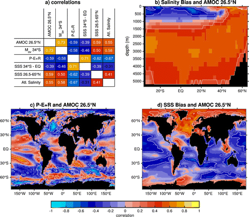
Figure 7. (a) Correlations between AMOC at 26.5°N, at 34°S, integrated freshwater fluxes from Bering Strait to 34°S (
), South Atlantic SSS bias (SSS 34°S-EQ), North Atlantic SSS bias (SSS 26.5-65°N) and salinity bias in the full depth Atlantic from 34°S-65°N (Atl. Salinity). (b–d) Spatial patterns of correlations between AMOC at 26.5°N and (b) Atlantic zonal mean salinity bias, (c)
, and (d) SSS bias. Statistically significant correlations at the 99% level are circled in white (b,c,d) or written in white text (a). Only the CMIP5 models which have surface freshwater fluxes available were used to compute
(See Table ).
Expanding the correlation analysis to the entire Atlantic basin shows that has a significant positive correlation with the strength of the AMOC at 26.5°N from the southern boundary of the Atlantic up to about 10°N, the southern boundary of the subtropical North Atlantic, where the correlation drops off drastically (Fig. a, blue). The correlation between
and the AMOC seems inversely related to the spread in
(compare Fig. a, blue and Fig. a). This suggests that further south the models possess compensating errors in AMOC strength and vertical velocity profile as they project on
, while north of 10°N the spread is dominated by errors in AMOC strength. However, the structure of the correlations changes significantly when comparing the salinity bias corrected
to the AMOC at 26.5°N (Fig. a, orange). Correlations are insignificant from 34°S to 10°N. This suggests that the significant correlation between the AMOC at 26.5°N and the uncorrected
in the South Atlantic occurs through the relationship between the AMOC and salinities rather than between the AMOC and the South Atlantic velocitiy field. Between 10–45°N there is a significant negative correlation between the AMOC and salinity bias corrected
(as expected since a stronger AMOC transports more salt northward at this latitude). If we instead consider the difference between
and the salinity bias corrected
(i.e. the transport of FW biases by the model velocity) correlated with the AMOC, this is statistically significant at all latitudes south of 45°N (Fig. a, yellow). Therefore, not only does the strength of the AMOC impact subtropical North Atlantic
directly, it also is related to
through a relationship with the salinity bias.
4. Role of atmospheric forcing
It is clear from Fig. c that on average there is a negative salinity bias in the upper few 100 m of the southern Atlantic. Estimated values for the total fresh water input from the surface fluxes () between the Bering Straight and 24°S, 26.5°N and 36°N are available from Bryden et al. (Citation2011), McDonagh et al. (Citation2010) and McDonagh et al. (Citation2015), respectively (Fig. ). For the integrated
at 34°S and 26.5°N the CMIP5 multi-model mean slightly underestimates the observational estimates, but the models’ values of the integrated
tend to fall within the possible range of the observational estimates (Fig. ). However, at 36°N the majority of the CMIP5 models lie outside the error bars of the estimated value of the integrated surface freshwater flux (Fig. ). This suggests that the models tend to overestimate the evaporation or underestimate the precipitation, particularly in the high latitude North Atlantic/Arctic. Initially, it may seem counterintuitive that models which evaporate too much or precipitate too little over the Atlantic have fresher surface waters in the Atlantic. However, for the entire Atlantic we see a strong positive salinity bias throughout the Atlantic basin at depth leading to a basin-averaged positive bias (Fig. c). The structure of the fresh bias at the surface is indicative of the Atlantic importing more freshwater to compensate for the salinification due to the negative bias in
, as the surface fresh bias is at its deepest at the southern boundary and decreases in depth farther north. This particular structure supports an
that is too positive in the southern Atlantic with a fresh bias in the northward moving waters and a salty bias in the deeper waters, which are transported southwards. Pardaens et al. (Citation2003) found that at 34°S during the spin-up of the coupled climate model, HadCM3, the
adjusted by increasing from a negative to a positive value to come into balance with the surface fluxes in the model, which featured too much evaporation over the Atlantic. Correcting the evaporative bias in the same model has been shown to improve the salinity bias and to change
from positive to negative (Jackson, Citation2013). But why are the models evaporating too much? Liu et al. (Citation2014) suggested that is was related to the incorrect representation of the Intertropical Convergence Zone (ITCZ). Also, models are known to have too much upwards latent heat fluxes in areas of stratocumulus cloud cover, especially in upwelling regions (Richter, Citation2015), implying too much evaporation.
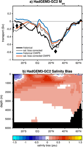
Figure 8. (a) The zonal values of for HadGEM3-GC2 for the historical mean (black) and the salinity bias corrected values (grey), and for the CMIP5 multi-model mean (blue) and salinity bias corrected multi-model mean (orange). Black markers indicate the same observational estimates as used in Fig. c. The zonal mean Atlantic salinity bias in HadGEM3-GC2.
The positive correlation between AMOC strength and at 34°S before correcting for salinity bias (Figs. a, c, and a) suggests a strong relationship between the AMOC and the model’s salinity bias. The correlation between the zonal mean salinity bias in the Atlantic and the AMOC at 26.5°N supports this; models with a stronger AMOC bringing in fresher water through the southern boundary of the Atlantic while the water at depth is more saline (Fig. b). Sea surface salinity (SSS) correlated with the AMOC also shows that a stronger AMOC has saltier surface waters in the North Atlantic/Arctic and fresher waters elsewhere (Fig. a and d). The
pattern related with the AMOC strength has a statistically significant negative correlation between
in the subpolar North Atlantic (Fig. c), a region just north of where the integrated
has the largest discrepancy with the observational estimates (Fig. ). The
integrated across the whole Atlantic shows a strong negative correlation with the SSS bias in the North Atlantic and the Atlantic as a whole (Fig. a). Wang et al. (Citation2014) showed that in the CMIP5 models the AMOC and the North Atlantic sea surface temperatures (SST) are positively correlated with a correlation of 0.85. Therefore, a model with a stronger AMOC, leads to warmer SSTs which encourages more evaporation, reflected in the correlation pattern of
with AMOC strength (Fig. c). The increase in evaporation salinifies the SSS in the North Atlantic leading to a positive correlation between North Atlantic SSS and the AMOC (Fig. a). Larger salinities at the surface of the North Atlantic decrease the stratification of the water column and this in turn supports a stronger AMOC. The combination of fresher surface water outside the Atlantic when the AMOC is stronger (Fig. d) and the stronger AMOC itself leads to an increased surface freshwater transport into the Atlantic and hence a more positive
at 34°S (Fig. a).
5. Conclusions and discussion
The value of at 34°S is often considered an indicator for AMOC bi-stability with a negative value indicating a bistable AMOC and positive values indicating a monostable AMOC. However, no rigorous proof for it’s relation with AMOC bi-stability exists. It’s value is motivated by Huisman et al. (Citation2010) and Sijp (Citation2012), who have investigated the relation between AMOC bi-stability and
from a salinity perturbation point of view. Both papers find that only the interaction between the mean salinity field and perturbations on the meridional flow can lead to instability of the AMOC on state. This occurs only when the (transport weighted) vertical salinity difference at 34°S is positive (that is, the salinity integrated between 0–1000 m must be larger than the salinity integrated between 1000–4500 m) and the AMOC therefore exports fresh water (imports salt). Observational estimates of
at 34°S suggest that the current climate system is in a bi-stable AMOC regime, since the vertical salinity difference at 34°S is indeed positive. From the analysis in this paper, we have seen that the models in CMIP5 for the most part have values of
at 34°S that are too positive, putting them in a monostable AMOC regime. However,
at 34°S is strongly affected by the salinity bias in the models. This salinity bias is mainly confined to the southern parts of the Atlantic due to a too evaporative North Atlantic basin which causes an anomalous freshwater import in the surface layers of the South Atlantic, which is then transported northward to compensate for the evaporative bias. The fresh anomaly at the surface is strongly correlated to the strength of the AMOC, suggesting that a too strong AMOC enhances the chance of a model falling into a monostable AMOC regime. After correcting the salinity bias,
changes sign and becomes negative for all models. The ensemble mean value changes from plus 0.09 to –0.19 Sv.
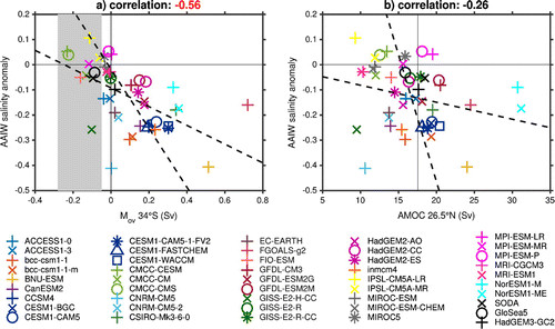
Figure 9. Same as Fig. but showing the mean salinity bias in the AAIW formation region (130°W-45°W, 60°S-50°S, upper 1000 m) and (a) at 34°S and (b) AMOC at 26.5°N.
The cause of the difference in from the observational estimates in the subtropical North Atlantic is more difficult to establish. Correcting for salinity biases has less impact as the salinity bias is more uniform with depth in the North Atlantic. Also velocity biases are important here. At 26.5°N the uncorrected value for
was –0.55 Sv, while after applying the velocity bias correction it becomes –0.67 Sv. One of the reasons for velocity biases might be that eddies play an important role in the total freshwater budget and they are underestimated in coarse resolution models (Tréguier et al., Citation2012; Mecking et al., Citation2016). The latter study also found that freshwater transport by the gyre can become much stronger in an eddy-permitting model, allowing for a stronger negative
.
In the study Mecking et al. (Citation2016) the eddy-permitting coupled climate model HadGEM3-GC2 was used in a hosing experiment. In this experiment, the model was held at present day climate conditions while freshwater hosing was applied to the North Atlantic and Arctic oceans which caused the AMOC circulation to collapse after only a few years. After 10 years of freshwater hosing (totalling 100 Sv*years of freshwater) the hosing was switched off and the model was allowed to run for another 450 years. During these 450 years the AMOC only experiences a weak recovery, barely exceeding 5 Sv, without the generation of a reverse overturning circulation. at 34°S in the present day control simulation of this model is weakly negative suggesting a bistable AMOC (Mecking et al., Citation2016) while in the historical simulation of HadGEM3-GC2 the value of
at 34°S is 0.02 Sv (Table , Fig. a). This suggests that HadGEM3-GC2 is on the boundary of a monostable and bistable AMOC according to the
at 34°S. HadGEM3-GC2 has a negative salinity bias in the southern Atlantic but only from 34°S to 20°S, north of which it is too saline (Fig. b), making it stand out from the CMIP5 models. In HadGEM3-GC2 this leads to a salinity bias corrected
which is more negative up to 20°S and more positive from 20°S to 26.5°N compared to the uncorrected
(Fig. a). At 26.5°N the
for HadGEM3-GC2 is –0.65 Sv making it closer to observational estimates then the multi-model mean of the CMIP5 models and both reanalysis products, with only 11 CMIP5 models having values closer to observations (Table , Fig. b). In general, HadGEM3-GC2 is an improvement compared to the average CMIP5 model and it was able to sustain a stable AMOC off state.
Yin and Stouffer (Citation2007) proposed a mechanism for AMOC bi-stability which involves the convergence of freshwater transport by the AMOC into the North Atlantic subtropical gyre. When the AMOC collapses, the reduction in northwards heat transport changes the sea surface temperature gradient which shifts the ITCZ southward. This results in less precipitation falling over the equatorial/subtropical North Atlantic and hence a saline anomaly in the subtropical North Atlantic develops. This increase in salinity in the subtropical North Atlantic, unless it is balanced by an increase in freshwater transport into this region, will destabilise the AMOC off state, leading to a recovery towards the AMOC on state. In the models analysed in Yin and Stouffer (Citation2007) the model which remained in the AMOC off state (GFDL R30) developed a RTHC cell which advected the necessary freshwater into the subtropical North Atlantic to counteract this salinification. While the higher resolution model (GFDL CM2.1) did not develop RTHC and the AMOC began to recover shortly after the hosing was applied. This suggested that the RTHC is essential for maintaining an AMOC off state in a coupled climate model. However, in HadGEM3-GC2 the AMOC off state was maintained for 450 years without the development of an RTHC (Mecking et al., Citation2016).
A budget analysis showed that in HadGEM3-GC2 the anomalous freshwater transport into the subtropical North Atlantic from was sufficient to counteract the salinification. In the historical simulation of HadGEM3-GC2 the freshwater transport divergence by the AMOC across the subtropical North Atlantic is –0.17 Sv (
at 10°N minus
at 45°N), which, when the AMOC collapses, leads to a large anomalous freshwater import into the subtropical North Atlantic, strong enough to counteract the salinification due to the shift in ITCZ. In the CMIP5 models, the freshwater transport divergence across the subtropical North Atlantic ranges from –0.01 Sv to 0.38 Sv, with a mean of 0.17 Sv, which, after an AMOC collapse, would not be sufficient to counteract a salinification of 0.05 Sv to 0.12 Sv from the changes in
(Yin and Stouffer, Citation2007; Mecking et al., Citation2016). Correcting for the salinity bias makes the freshwater transport divergence slightly more negative from the CMIP5 models with a mean of 0.03 Sv, still not sufficient to counteract the salinification. Both SODA (0.08 Sv) and GloSea5 (0.05 Sv) have a freshwater transport divergence closer to the CMIP5 values than the negative value in HadGEM3-GC2. In HadGEM3-GC2, the freshwater transport divergence by the AMOC across the subtropical Atlantic becomes more positive after a correction of the salinity bias, suggesting that HadGEM3-GC2 overestimated the salt advection into the subtropical North Atlantic. However, since we do not have observations of the AMOC or
at 10°N and 45°N, we cannot quantify the effect of the velocity bias on the freshwater transport divergence by the AMOC and hence we cannot assess which model is more accurate.
For a stable AMOC off state to occur one of two things needs to happen; 1) the divergence of across the subtropical North Atlantic needs to be negative enough in the AMOC off state or 2) a RTHC needs to develop when the AMOC collapses, bringing in the extra freshwater needed. The reanalysis products and the CMIP5 models suggest that the first is unlikely, hence the generation of a RTHC is required. For the RTHC to develop a positive density difference between the region of Antarctic Intermediate Water (AAIW) formation and the NADW formation regions are needed after the AMOC has collapsed (Saenko et al., Citation2003; Yin and Stouffer, Citation2007). In the majority of the models there is a negative surface salinity bias in the South Atlantic which extends to the northern part of the Southern Ocean, resulting in less dense water in the AAIW formation region. These fresher AAIWs are then transported into the Atlantic making
at 34°S more positive while having no significant link with the AMOC strength (Fig. ). Therefore, with the AAIW formation region being too fresh, when the AMOC collapses due to a freshening of the NADW formation region, this freshening is not enough to create the reverse density gradient required for the generation of an RTHC. The likely reason why the RTHC appeared in the GFDL R30 model (Yin and Stouffer, Citation2007) was due to the salinity biases being reduced through flux adjustment. Therefore, reducing the negative surface salinity bias in the southern Atlantic would make it more likely for an RTHC to develop during an AMOC collapse, as well as bringing the values of
at 34°S closer to the observational estimates.
Acknowledgements
We acknowledge the World Climate Research Programme’s Working Group on Coupled Modelling, which is responsible for CMIP, and we thank the climate modelling groups (listed in Table 1 of this paper) for producing and making available their model output. For CMIP the US Department of Energy’s Program for Climate Model Diagnosis and Intercomparison provides coordinating support and led development of software infrastructure in partnership with the Global Organization for Earth System Science Portals. Some of the computations were preformed on JASMIN, a super-data-cluster which we are thankful to have been allowed to use (Lawrence et al., Citation2013). We would also like to thank Drew Peterson for allowing us to use the GloSea5 data in our analysis. We would like to acknowledge Jeff Blundell and Adam Blaker for their technical help and useful conversations. And finally, we acknowledge Jan Sedáček and Michael Eby for discussions about the computations of at 34°S in Weaver et al. (Citation2012).
Notes
No potential conflict of interest was reported by the authors.
References
- Blunier, T. and Brook, E. J. 2001. Timing of millennial-scale climate change in Antarctica and Greenland during the last glacial period. Science 291, 109–112. DOI: 10.1126/science.291.5501.109.
- Broecker, W. S., Bond, G., Klas, M., Bonani, G. and Wolfli, W. 1990. A salt oscillator in the glacial Atlantic? 1. The concept. Paleoceanography 5, 469–477.
- Bryden, H. L., King, B. A. and McCarthy, G. D. 2011. South Atlantic overturning circulation at 24 S. J. Mar. Res. 69, 38–55. DOI: 10.1357/002224011798147633.
- Carton, J. A. and Giese, B. S. 2008. A reanalysis of ocean climate using Simple Ocean Data Assimilation (SODA). Mon. Weather Rev. 136, 2999–3017. DOI: 10.1175/2007MWR1978.1.
- Collins, M., Knutti, R., Arblaster, J., Dufresne, J. L., Fichefet, T., and co-authors. 2013. Long-term climate change: Projections, commitments and irreversibility. In: Climate Change 2013: The Physical Science Basis. Contribution of Working Group I to the Fifth Assessment Report of the Intergovernmental Panel on Climate Change (eds. T.F. Stocker, D. Qin, G.-K. Plattner, M. Tignor, S. K. Allen, J. Boschung, A. Nauels, Y. Xia, V. Bex and P. M. Midgley). book section Vol. 12, Cambridge University Press, Cambridge, United Kingdom and New York, NY, USA, pp. 1029–1136. DOI: 10.1017/CBO9781107415324.024. Online at: www.climatechange2013.org
- Danabasoglu, G., Yeager, S. G., Bailey, D., Behrens, E., Bentsen, M. and co-authors. 2014. North Atlantic simulations in coordinated ocean-ice reference experiments phase II (CORE-II). Part I: Mean States. Ocean Modell. 73, 76–107. DOI: 10.1016/j.ocemod.2013.10.005.
- Dansgaard, W., Johnsen, S. J., Clausen, H. B., Dahl-Jensen, D., Gundestrup, N. S. and co-authors. 1993. Evidence for general instability of past climate from a 250-kyr ice-core record. Nature 364, 218–220. DOI:10.1038/364218a0.
- de Abreu, L., Shackleton, N. J., Schönfeld, J., Hall, M. and Chapman, M. 2003. Millennial-scale oceanic climate variability off the Western Iberian margin during the last two glacial periods. Mar. Geol. 196, 1–20. DOI:10.1016/S0025-3227(03)00046-X.
- de Vries, P. and Weber, S. L. 2005. The Atlantic freshwater budget as a diagnostic for the existence of a stable shut down of the meridional overturning circulation. Geophys. Res. Lett. 32, DOI: 10.1029/2004GL021450.
- Drijfhout, S. S., Weber, S. L. and van der Swaluw, E. 2011. The stability of the MOC as diagnosed from model projections for pre-industrial, present and future climates. Clim. Dyn. 37(7–8), 1575–1586. DOI: 10.1007/s00382-010-0930-z.
- Garzoli, S. L., Baringer, M. O., Dong, S., Perez, R. C. and Yao, Q. 2013. South Atlantic meridional fluxes. Deep Sea Res. Part I 71, 21–32. DOI: 10.1016/j.dsr.2012.09.003.
- Hansen, J., Sato, M., Hearty, P., Ruedy, R., Kelley, M. and co-authors. 2016. Ice melt, sea level rise and superstorms: Evidence from paleoclimate data, climate modeling, and modern observations that 2 C global warming could be dangerous. Atmos. Chem. Phys. 16, 3761–3812. DOI: 10.5194/acp-16-3761-2016.
- Huisman, S. E., Den Toom, M., Dijkstra, H. A. and Drijfhout, S. 2010. An indicator of the multiple equilibria regime of the Atlantic meridional overturning circulation. J. Phys. Oceanogr. 40, 551–567. DOI: 10.1175/2009JPO4215.1.
- Ingleby, B. and Huddleston, M. 2007. Quality control of ocean temperature and salinity profiles: Historical and real-time data. J. Mar. Syst. 65, 158–175. DOI: 10.1016/j.jmarsys.2005.11.019.
- Jackson, L. 2013. Shutdown and recovery of the AMOC in a coupled global climate model: the role of the advective feedback. Geophys. Res. Lett. 40, 1182–1188. DOI: 10.1002/grl.50289.
- Jackson, L., Kahana, R., Graham, T., Ringer, M. A., Woollings, T. and co-authors. 2015. Global and European climate impacts of a slowdown of the AMOC in a high resolution GCM. Clim. Dyn. 45, 3299–3316. DOI: 10.1007/s00382-015-2540-2.
- Jackson, L. C., Peterson, K. A., Roberts, C. D. and Wood, R. A. 2016. Recent slowing of Atlantic overturning circulation as a recovery from earlier strengthening. Nat. Geosci. 9, 518–522. DOI: 10.1038/ngeo2715.
- Lawrence, B. N., Churchill, J., Juckes, M., Kershaw, P., Pascoe, S. and co-authors. 2013. Storing and manipulating environmental big data with jasmin. In: 2013 IEEE International Conference on Big Data, IEEE, Santa Clara, CA, pp. 68–75. DOI: 10.1109/BigData.6691556.
- Liu, W. and Liu, Z. 2013. A diagnostic indicator of the stability of the Atlantic meridional overturning circulation in CCSM3. J. Clim. 26, 1926–1938. DOI: 10.1175/JCLI-D-11-00681.1.
- Liu, W., Liu, Z. and Brady, E. C. 2014. Why is the AMOC monostable in coupled general circulation models? J. Clim. 27, 2427–2443. DOI: 10.1175/JCLI-D-13-00264.1.
- Liu, W., Xie, S. P., Liu, Z. and Zhu, J. 2017. Overlooked possibility of a collapsed atlantic meridional overturning circulation in warming climate. Sci. Adv. 3, 1601–666. DOI: 10.1126/sciadv.1601666.
- Madec, G. 2008. NEMO Ocean Engine, Institut Pierre-Simon Laplace (IPSL), France.
- Manabe, S. and Stouffer, R. 1988. Two stable equilibria of a coupled ocean-atmosphere model. J. Clim. 1, 841–866. DOI: 10.1175/1520-0442.
- Marotzke, J. 1990. Instabilities and multiple equilibria of the thermohaline circulation. PhD thesis. Christian-Albrechts-Universit{\"a}t.
- McDonagh, E. L., King, B. A., Bryden, H. L., Courtois, P., Szuts, Z. and co-authors. 2015. Continuous estimate of Atlantic oceanic freshwater flux at 26.5? n. J. Clim. 28, 8888–8906. DOI: 10.1175/JCLI-D-14-00519.1.
- McDonagh, E. L. and King, B. A. 2005. Oceanic fluxes in the South Atlantic. J. Phys. Oceanogr. 35, 109–122. DOI: 10.1175/JPO-2666.1.
- McDonagh, E. L., McLeod, P., King, B. A., Bryden, H. L. and Valdés, S. T. 2010. Circulation, heat, and freshwater transport at 36 N in the Atlantic. J. Phys. Oceanogr. 40, 2661–2678. DOI: 10.1175/2010JPO4176.1.
- Mecking, J., Drijfhout, S., Jackson, L. and Graham, T. 2016. Stable AMOC off state in an eddy-permitting coupled climate model. Clim. Dyn. 47, 2455–2470. DOI: 10.1007/s00382-016-2975-0.
- Megann, A., Storkey, D., Aksenov, Y., Alderson, S., Calvert, D. and co-authors. 2014. GO5. 0: The joint NERC-Met Office NEMO global ocean model for use in coupled and forced applications. Geosci. Model Dev. 7, 1069–1092. DOI: 10.5194/gmd-7-1069-2014.
- Pardaens, A., Banks, H., Gregory, J. and Rowntree, P. 2003. Freshwater transports in hadcm3. Clim. Dyn. 21, 177–195. DOI: 10.1007/s00382-003-0324-6.
- Rahmstorf, S. 1996. On the freshwater forcing and transport of the Atlantic thermohaline circulation. Clim. Dyn. 12, 799–811. DOI: 10.1007/s003820050144.
- Reintges, A., Martin, T., Latif, M. and Keenlyside, N. S. 2016. Uncertainty in twenty-first century projections of the Atlantic Meridional Overturning Circulation in CMIP3 and CMIP5 models. Clim. Dyn. 1–17. DOI: 10.1007/s00382-016-3180.
- Richter, I. 2015. Climate model biases in the eastern tropical oceans: Causes, impacts and ways forward. Wiley Interdiscip. Rev. Clim. Change 6, 345–358. DOI: 10.1002/wcc.338.
- Saenko, O. A., Weaver, A. J. and Gregory, J. M. 2003. On the link between the two modes of the ocean thermohaline circulation and the formation of global-scale water masses. J. Clim. 16, 2797–2801. DOI: 10.1175/1520-0442(2003)016<2797:OTLBTT>2.0.CO;2.
- Sijp, W. P. 2012. Characterising meridional overturning bistability using a minimal set of state variables. Clim. Dyn. 39, 2127–2142. DOI: 10.1007/s00382-011-1249-0.
- Smeed, D., McCarthy, G., Cunningham, S. A., Frajka-Williams, E., Rayner, D. and co-authors. 2014. Observed decline of the Atlanticmeridional overturning circulation 2004–2012. Ocean Sci. 10, 29–38. DOI: 10.5194/os-10-29-2014.
- Smeed, D., et al. 2015. Atlantic meridional overturning circulation observed by the RAPID-MOCHA-WBTS (RAPID-Meridional Overturning Circulation and Heatflux Array-Western Boundary Time Series) array at 26N from 2004 to British Oceanographic Data Centre -- Natural Environment Research Council, UK. DOI: 10.5285/1a774e53-7383-2e9a-e053-6c86abc0d8c7.
- Stommel, H. 1961. Thermohaline convection with two stable regimes of flow. Tellus 13, 224–230.
- Stouffer, R. J., Smeed, D., McCarthy, G., Rayner, D., Moat, B. I. and co-authors. 2006. Investigating the causes of the response of the thermohaline circulation to past and future climate changes. J. Clim. 19, 1365–1387. DOI: 10.1175/JCLI3689.1.
- Taylor, K. E., Stouffer, R. J. and Meehl, G. A. 2012. An overview of CMIP5 and the experiment design. Bull. Am. Meteorol. Soc. 93, 485–498. DOI: 10.1175/BAMS-D-11-00094.1.
- Tréguier, A. M., Deshayes, J., Lique, C., Dussin, R. and Molines, J. M. 2012. Eddy contributions to the meridional transport of salt in the North Atlantic. J. Geophys. Res. Oceans 117, 978–2012. DOI: 10.1029/2012JC007927.
- Valdes, P. 2011. Built for stability. Nature Geosci. 4, 414–416.
- Vellinga, M. and Wood, R. A. 2002. Global climatic impacts of a collapse of the Atlantic thermohaline circulation. Clim. Change 54, 251–267. DOI: 10.1023/A:1016168827653.
- Wang, C., Zhang, L., Lee, S. K., Wu, L. and Mechoso, C. R. 2014. A global perspective on CMIP5 climate model biases. Nat. Clim. Change 4, 201–205. DOI: 10.1038/NCLIMATE2118.
- Weaver, A. J., Sedláček, J., Eby, M., Alexander, K., Crespin, E. and co-authors. 2012. Stability of the Atlantic meridional overturning circulation: A model intercomparison. Geophys. Res. Lett. 39, DOI: 10.1029/2012GL053763.
- Williams, K., Williams, K. D., Harris, C. M., Bodas-Salcedo, A., Camp, J. and co-authors. 2015. The Met Office Global Coupled model 2.0 (GC2) configuration. Geosci. Model Dev. 8, 1509–1524. DOI: 10.5194/gmd-8-1509-2015.
- Yin, J. and Stouffer, R. J. 2007. Comparison of the stability of the Atlantic thermohaline circulation in two coupled atmosphere-ocean general circulation models. J. Clim. 20, 4293–4315. DOI: 10.1175/JCLI4256.1.
