Long-term variations of the mole fraction and carbon isotope ratio of atmospheric methane observed at Ny-Ålesund, Svalbard from 1996 to 2013

The data presented in this paper are downloadable from the website (http://caos.sakura.ne.jp/tgr/data/en).

Abstract

We have conducted systematic observations of the CH₄ mole fraction and its carbon isotope ratio (δ¹³C) at Ny-Ålesund, Svalbard (78°55′N, 11°56′E) using air samples collected weekly since 1991 and 1996, respectively. The CH₄ mole fraction showed long-term increase until 1999, stagnation between 2000 and 2006, followed by an increase after 2006. On the other hand, δ¹³C showed monotonous increase until 2006 and decrease after 2006. By comparing the rates of change in the CH₄ mole fraction and δ¹³C under the assumption that the atmospheric CH₄ lifetime is constant, it is suggested that the temporal pause of the CH₄ mole fraction observed at Ny-Ålesund is attributed to reductions of CH₄ release from the microbial and fossil fuel sectors. On the other hand, the increase in CH₄ after 2006 could be ascribed to an increase in microbial CH₄ release. The CH₄ and δ¹³C data presented in this paper would be useful for clarifying their temporal variations in the Arctic atmosphere, as well as providing additional constraints on the global CH₄ budget.

Keywords:

• atmospheric methane
• stable carbon isotope
• greenhouse gas
• Arctic

1. Introduction

Atmospheric CH₄ is one of the most important gases for the atmospheric greenhouse effect and the atmospheric chemistry (Saunois et al., 2016). To predict future climate change more precisely, characterizing variations in the CH₄ sources and sinks and their response to climate variability is indispensable. Systematic observations of the atmospheric CH₄ mole fractions since the 1980s revealed that the mole fraction significantly increased in the 1980s and the 1990s, stabilized globally around 2000 and then increased again from 2006 to the present (Rigby et al., 2008; Dlugokencky et al., 2009). However, since many CH₄ sources are distributed inhomogeneously throughout the globe and their respective contributions to atmospheric CH₄ are difficult to distinguish using observations of the atmospheric CH₄ mole fraction alone, the source(s) responsible for the long-term CH₄ variations have not been clearly identified yet (Saunois et al., 2016). In addition, the temporal change in the CH₄ removal rate, which occurs mainly through reaction with the OH radical, is not quantitatively well understood (Dalsøren et al., 2016).

The stable carbon isotope of atmospheric CH₄ (δ¹³C relative to V-PDB) provides us with additional information for understanding the CH₄ cycle, as each source category, microbial, fossil fuel and biomass burning, has a characteristic δ¹³C value of ~−60, ~−40 and ~−25‰, respectively (Whiticar and Schaefer, 2007). Recently, Schaefer et al. (2016) compiled global δ¹³C data observed by five institutions and analysed them using a box model. They found that the behaviour of CH₄, which stabilized after 1999 and increased again after 2006, could be a result of a reduced fossil fuel source and enhanced microbial source, respectively. Nisbet et al. (2016) also analysed their own δ¹³C data together with those from the National Oceanic and Atmospheric Administration and Institute of Arctic and Alpine Research, University of Colorado (NOAA/INSTAAR) (White et al., 2015), which indicated that the increase in the release of CH₄ from wetlands was responsible for the CH₄ regrowth after 2006. However, the institutions conducting systematic δ¹³C observations are still limited and the δ¹³C data are sparse. For more detailed investigation of the variations in atmospheric CH₄, additional and independent δ¹³C data are required.

We have continued systematic observations of the CH₄ mole fraction and δ¹³C of CH₄ using air samples collected at Ny-Ålesund, Svalbard since 1991 and 1996, respectively (Morimoto et al., 2006). In this paper, we present long-term variations of the CH₄ mole fraction and δ¹³C at Ny-Ålesund until the end of 2013 and discuss the causes of the atmospheric CH₄ variations based on the δ¹³C data.

2. Experimental procedures

Weekly air sampling began at the Japanese observatory at Ny-Ålesund, Svalbard in 1991 in cooperation with the Norwegian Polar Institute, and sample analyses of the CH₄ mole fraction and δ¹³C have been conducted at our laboratory in Japan since 1991 and 1996, respectively. The sampling site is 40 m above sea level and about 2.6 km north of Zeppelin station where air samples have been collected for the NOAA/Global Monitoring Division (NOAA/GMD). Since details of our air sampling and analysis procedures for the CH₄ mole fraction and δ¹³C have already been given (Aoki et al., 1992; Morimoto et al., 2006, 2009), only a brief explanation is presented here.

The CH₄ mole fraction was determined against our standard gas scale maintained at Tohoku University using a gas chromatograph (GC) equipped with a flame ionization detector (Aoki et al., 1992). From repetitive calibration of the CH₄-in-air standard gases, the repeatability of our CH₄ mole fraction measurement was estimated to be within 1.0 ppb (one standard deviation [1 s.d.]). In this paper, the CH₄ mole fraction is expressed as ‘ppb’, which has the same meaning as ‘nmol mol⁻¹’. δ¹³C of CH₄ was determined by using a GC-Combustion-Isotope Ratio Mass Spectrometer (IRMS) based on MAT-252 (Thermo Fischer). The repeatability of our δ¹³C analysis was determined to be within 0.13‰ (1 s.d.) by replicate analyses of our CH₄-in-air ‘test gas’ between June 2000 and September 2001, and then improved to 0.08‰ in September 2001 and further to 0.06‰ in August 2002 (Morimoto et al., 2006). The air samples collected before June 2000 were analysed when the repeatability was 0.08‰. An intercomparison of the δ¹³C scale with the National Institute of Water and Atmosphere (NIWA), New Zealand, conducted in 2004, showed that our scale was heavier than the NIWA scale by 0.33 ± 0.04‰. This number is different from that reported by Morimoto et al. (2006), since the data conversion from our internal scale to the V-PDB scale was updated. The internal consistency of our δ¹³C analyses over a long period of time was confirmed by analysing ‘check gas’ with the known δ¹³C value every analysis day. In addition, we have maintained five CH₄-in-air standard gases of which δ¹³C values were determined against V-PDB. By comparing them periodically, we confirmed that their mutual relationship was invariant during the period covered by this observation.

3. Results and discussion

Figure 1a and b show the CH₄ mole fractions and δ¹³C values observed at Ny-Ålesund, respectively, along with their best-fit curves and long-term trends, obtained by using a digital-filtering technique (Nakazawa et al., 1997). In the curve fitting procedure, the cut-off period of the low-pass filter was set to four months to derive the best-fit curves to the data and to five years to extract the long-term trends. As described in Nakazawa et al. (1997) in detail, the digital-filtering method employed in this study never causes the phase shift in finally obtained output signals, since the output from the filter is reversed and then passed through the filter again to compensate for the phase shift.

Fig. 1. Temporal variations of the CH₄ mole fraction (a) and δ¹³C of CH₄ (b) observed at Ny-Ålesund, Svalbard. Also shown are their best-fit curves (solid lines) and long-term trends (broken lines).

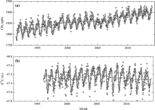
As seen in the figures, the CH₄ mole fraction and δ¹³C showed clear seasonal cycles superimposed on the long-term trends. Average peak-to-peak amplitudes of the CH₄ and δ¹³C seasonal cycles are 45 ppb and 0.44‰, respectively. The amplitudes and seasonal phase are similar to those previously reported (Morimoto et al., 2006). The CH₄ mole fraction increased from 1991 to 2000, stagnated until around 2006, and then resumed increasing at a similar rate as the 1990s after 2006. Such a stepwise CH₄ increase has also been observed around the world (Rigby et al., 2008; Dlugokencky et al., 2009). The CH₄ variations observed at Ny-Ålesund are similar to those at Alert and Barrow by NOAA/GMD (Dlugokencky et al., 2016). On the other hand, δ¹³C observed at Ny-Ålesund shows a continuous increase from 1996 to around 2006 and a decrease afterwards, with smaller temporal variability than at Alert (White et al., 2015).

For a close examination of the CH₄ trend changes around 2000 and 2006, a stepwise line fitting (Reinsel et al., 2002), assuming slope change at two points, was applied to the long-term component of CH₄ derived by the digital filtering. We selected 2000.8 and 2005.8 (decimal year; hereinafter the same expression is used) as the points where the slope changed to minimize the sum of squared residuals of the stepwise fitting. To evaluate the standard error of the average rate of increase due to short-term CH₄ variations and/or measurement error, we conducted a residual bootstrap analysis with 5000 pseudo time series of the CH₄ mole fraction. The stepwise linear fitting and bootstrap analysis were also applied to the δ¹³C data with the same set-up as above. Figure 2 shows the long-term components of the observed CH₄ mole fraction and δ¹³C, along with the lines derived by the stepwise fitting. The average rates of increase in the CH₄ mole fraction and δ¹³C for each segment are listed in Table 1, along with their standard errors and 95% confidence intervals. The average rate of increase depends on where the points of slope change are set, as well as on how the cut-off period of the digital filter is chosen to extract the long-term component from the observed time series. To examine the sensitivity of the rate of increase on the given points, we calculated the rate of increase by shifting the two points by ±0.5 years around 2000.8 and 2005.8, respectively. The result indicated that the changes in the rate of increase were within the standard errors, obtained by the bootstrap analysis, shown in Table 1. We further calculated the average rates of increase in the CH₄ mole fraction and δ¹³C from the long-term component extracted with the cut-off period of 2 years. As a result, we confirmed that the stiffness of the digital filter does not affect the conclusion of this study.

Fig. 2. Long-term components of the CH₄ mole fraction (a) and δ¹³C (b) at Ny-Ålesund, Svalbard obtained by using the digital filtering technique in which the cut-off period was set to 5 years. Also shown are the regression lines for each segment obtained by the stepwise fitting, given the points of slope change at 2000.8 and 2005.8 (decimal year).

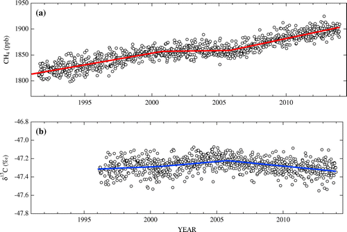
Table 1. The average rate of increase in CH₄ (ppb yr⁻¹) (a) and δ¹³C (‰ yr⁻¹) (b) for given periods, together with their respective standard errors (s.e.) and 95% confidence intervals (C.I.) obtained using the bootstrap analysis.

Period	Increase rate	s.e.	95% C.I.
(a)
1991.0–2000.8	4.5	0.2	[4.2, 4.8]
2000.8–2005.8	0.3	0.2	[–0.1, 0.8]
2005.8–2014.0	5.5	0.2	[5.1, 5.8]
(b)
1996.0–2000.8	0.006	0.003	[0.000, 0.012]
2000.8–2005.8	0.012	0.002	[0.008, 0.017]
2005.8–2014.0	−0.014	0.005	[–0.024, −0.004]

The atmospheric CH₄ mole fraction is determined by a balance between the CH₄ released from sources and CH₄ removal, mainly through reaction with the OH radical. In previous studies, the CH₄ removal rate was estimated by atmospheric chemistry models and forward/inversion calculations, with proxies such as methyl chloroform (CH₃CCl₃) (e.g. Spivakovsky et al., 2000; Montzka et al., 2011; Voulgarakis et al., 2013; Patra et al., 2014). Recently, McNorton et al. (2016) derived temporal variations of the atmospheric OH by analysing CH₃CCl₃ data with a box model, and proposed that small variations in OH played an important role in the stagnation of the CH₄ mole fraction between 1999 and 2006. Rigby et al. (2017) and Turner et al. (2017) also suggested, from their inversion calculations of CH₃CCl₃, CH₄ and δ¹³C of CH₄, that fluctuations in the CH₄ removal rate, as well as an increase in CH₄ emissions from the 2000s, are responsible for the CH₄ stagnation in the early 2000s and the regrowth after 2007. In spite of these studies, we analysed our observed CH₄ trend in terms of CH₄ sources, considering that there still remain uncertainties in the long-term trend and interannual variations of the CH₄ removal rate (Dalsøren et al., 2016). If the assumption that the atmospheric OH is invariant is not the case, the results obtained in this analysis would be modified to some extent. To include potential effects arisen from the OH radical, further observations and modelling studies on quantification of its temporal variations are required.

3.1. CH₄ levelling off from 2000 to 2006

As shown in Table 1, the average rate of increase in the CH₄ mole fraction observed at Ny-Ålesund decreased from 4.5 ± 0.2 ppb yr⁻¹ (one standard error, [1 s.e.]) in the period of 1991.0–2000.8 to 0.3 ± 0.2 ppb yr⁻¹ in 2000.8–2005.8, the rate of increase differing by 4.2 ppb yr⁻¹ between the two periods. Such a stepwise change in the rate of increase was observed globally (Dlugokencky et al., 2009), and the global average rate of increase calculated from the NOAA/GMD global data from 2000 to 2006 was 0.4 ± 3.1 ppb yr⁻¹ (1 s.d.). On the other hand, the rate of increase in δ¹³C observed at Ny-Ålesund showed a small value of 0.006 ± 0.003‰ yr⁻¹ (1 s.e.) for 1996.0–2000.8 and 0.012 ± 0.002‰ yr⁻¹ for 2000.8–2005.8. Schaefer et al. (2016) reported that the global average δ¹³C constructed from the data at 17 sites by 5 institutions increased until 1999 and then levelled off until the end of 2006. The δ¹³C data at the northern mid-latitudes used by Rice et al. (2016) showed a long-term increase at an average rate of +0.022 ± 0.027‰ yr⁻¹ in the 1990s and a stabilization to a rate of –0.01 ± 0.027‰ yr⁻¹ in 2000–2010. The difference between the rates of change in δ¹³C obtained at Ny-Ålesund and by Rice et al. (2016) could be partly due to the different periods in the respective slope calculations.

Dlugokencky et al. (2003) reported that the annual increase rate of the globally-averaged CH₄ mole fraction decreased with time from the beginning of their observation in 1984 until 2002, suggesting that the CH₄ budget is heading toward steady state, if the lifetime of atmospheric CH₄ is constant. On the other hand, Schaefer et al. (2016) showed from their box-model simulations that the CH₄ increase rate gradually decreased when a constant CH₄ emission (steady state) is assumed after 1992 and that the CH₄ emission should be reduced temporally to reproduce the observed CH₄ variations by the model. Considering that our observation period is close to that in Schaefer et al. (2016), we assume in the following discussion that the decline in the rate of increase in the CH₄ mole fraction around 2000.8 is due to changes in the CH₄ budget, rather than due to an approach to steady state.

To evaluate the aggregated δ¹³C value of the CH₄ sources that caused the CH₄ slope change at Ny-Ålesund at 2000.8, we employed the formulation presented by Lassey et al. (2000) and simplified it as:

(1)

where δ_source is the average δ¹³C of contributing CH₄ sources, and are the rates of change in the δ¹³C and CH₄ slopes before and after 2000.8, respectively, and C and δ_a denote the observed atmospheric CH₄ mole fraction and δ¹³C at 2000.8, respectively. By substituting the numbers given in Table 1 into Equation (1), we obtained –50.2 ± 2.4‰ for δ_source. With this value CH₄ is isotopically heavier than biogenic CH₄ (–58 to –62‰) and lighter than CH₄ from fossil fuel (–37 to –44‰) and biomass burning (–7 to –27‰) (Whiticar and Schaefer, 2007). Recently, Schwietzke et al. (2016) estimated globally averaged δ¹³C of CH₄ from fossil fuel sources to be –44.0 ± 0.7‰. Their value is still higher than the δ_source obtained in this study. We did not find any significant trend in the CH₄ release from biomass burning for 1999–2014, by inspecting an updated version of (van der Werf et al., 2010) based on the Global Fire Emissions Database version 4 (GFED4s) (Giglio et al., 2013). Therefore, the flattening of the CH₄ increase observed at Ny-Ålesund after 2000.8 could be attributable to a simultaneous reduction in CH₄ release from biogenic and fossil fuel sources.

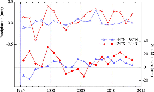
Figure 3 shows precipitation and soil moisture anomalies calculated at wetland and rice paddy regions in the tropics (24°N–24°S) and northern high latitudes (44–90°N) (Matthews and Fung, 2003), using CMAP Precipitation Data and CPC Soil Moisture Data (available from the websites given in References). In this calculation, possible inflow of precipitation in mountain areas to the two regions was assumed to be a small effect. As can be seen from this figure, precipitation and soil moisture in the tropics decreased in the first half of the 2000s. Considering that biogenic CH₄ production is enhanced with increasing water table depth (e.g. Wania et al., 2013), these decreasing trends are qualitatively consistent with a reduction in CH₄ emissions from wetlands and/or rice paddies, which are the dominant biogenic CH₄ sources. The intercomparison project of process-based models for wetland CH₄ emissions (WETCHIMP) gave widely variant results on the interannual variations in CH₄ release from wetlands (Wania et al., 2013). On the other hand, Zhu et al. (2015) showed that the CH₄ release from wetlands was reduced in 2000–2006 by using their process-based model.

Fig. 3. Yearly anomalies of precipitation (open circles and triangles) and soil moisture content (solid circles and triangles) calculated for wetland and rice paddy regions (Matthews and Fung, 2003) in 44–90°N and 24°S-24°N. Soil moisture is expressed as water equivalent depth.

Our observation data of CH₄ and δ¹³C at Ny-Ålesund indicate that the fossil fuel CH₄ source became weak at the beginning of the 2000s, in addition to the biogenic source, while Schaefer et al. (2016) suggested that the fossil fuel sector was a main contributor to the levelling off of CH₄ from 1993 to 2006. The different results between the two studies are arisen from the different temporal behaviours of δ¹³C. The global average trend of δ¹³C found by Schaefer et al. (2016) stagnated between 2000 and 2006; however, our data show a rather monotonous increase during the period. Atmospheric inversion studies by Bousquet et al. (2006) using CH₄ data and by Rice et al. (2016) using CH₄ and δ¹³C data showed an increase in fossil fuel CH₄ emission after 2000, coincident with a reduction in wetland emission. To balance the ¹³CH₄ budget in the atmosphere, they also required a reduction in the release of CH₄ from biomass burning during 1984–2009.

3.2. Regrowth of CH₄ after 2006

The average rate of increase in CH₄ observed at Ny-Ålesund increased from 0.3 ± 0.2 ppb yr⁻¹ for 2000.8–2005.8 to 5.5 ± 0.2 ppb yr⁻¹ for 2005.8–2014.0, as shown in Table 1, with a slope change of 5.1 ± 0.4 ppb yr⁻¹ at 2005.8. Our rate of increase after 2005.8 approximates the result of Rice et al. (2016) in which the average rate of increase of CH₄ at the northern mid-latitudes (35–48 °N) for 2006–2010 was 4.6 ± 1.3 ppb yr⁻¹ (95% confidence interval). On the other hand, the rate of increase of δ¹³C at Ny-Ålesund decreased from 0.012 ± 0.002‰ yr⁻¹ for 2000.8–2005.8 to –0.014 ± 0.005‰ yr⁻¹ for 2005.8–2014.0, with a slope change between the two periods of –0.027 ± 0.005‰ yr⁻¹. The δ¹³C rate of increase after 2005.8 is smaller than the globally averaged rate of –0.027‰ yr⁻¹ for 2006–2014, which was calculated from the data-set presented by Schaefer et al. (2016). This discrepancy would be due to latitudinally dependent rate of increase in δ¹³C, since δ¹³C had a more gentle temporal decrease in the northern high latitudes than in the southern hemisphere after 2006 (Schaefer et al., 2016). In fact, the δ¹³C rate of increase at Barrow and Alert for 2006–2014 were –0.019 ± 0.006 and –0.018 ± 0.009‰ yr⁻¹, respectively, which were calculated using the data tabulated in the supplemental information of Schaefer et al. (2016).

By using Equation (1) and the related rates of change shown in Table 1, the average δ¹³C value of CH₄ sources that enhanced the CH₄ increase at 2005.8 was estimated to be –56.9 ± 4.1‰. Considering that the CH₄ increase and δ¹³C decrease were steeper in 2005.8–2011.0 than after 2011.0, the stepwise fitting was applied again, which included the change in slope set at points 2000.8, 2005.8 and 2011.0. The source δ¹³C values were estimated by using Equation (1) to be –57.1 ± 4.9 and –58.0 ± 9.5‰ for 2005.8–2011.0 and 2011.0–2014.0, respectively. The values obtained for the two periods are close to each other, suggesting that microbial CH₄ played a dominant role in the CH₄ regrowth at Ny-Ålesund after 2006.

Several previous studies based on the δ¹³C observations also pointed out that biogenic sources are the main driver of the CH₄ regrowth after 2006 (Dlugokencky et al., 2009; Nisbet et al., 2016; Schaefer et al., 2016). However, it is difficult to understand only from the δ¹³C data which microbial source, wetland (Nisbet et al., 2016) or ruminant (Schaefer et al., 2016), contributed to what extent of the CH₄ regrowth. Since the precipitation shows large positive anomalies in 2006–2007 globally and tropical soil moisture was restored to pre-2000s levels after 2006, as shown in Fig. 3, the tropical wetlands and/or rice paddies are responsible for the CH₄ regrowth after 2006 to some extent.

There still exists disagreement about the cause of the CH₄ regrowth after 2006. Several studies claimed that CH₄ from fossil fuels increased continuously after 2007 (Bergamaschi et al., 2013; Helmig et al., 2016; Hausmann et al., 2016; Kirschke et al., 2013). As already suggested by Schaefer et al. (2016), additional CH₄ input to the atmosphere from fossil fuel sources requires a concurrent reduction in the CH₄ release from isotopically heavier sources, such as biomass burning, to balance the ¹³CH₄ budget in the atmosphere. To understand the CH₄ regrowth after 2006 in more detail, further studies including inventory, process-based modelling and top-down approaches are required.

4. Concluding remarks

We have conducted systematic observations of the CH₄ mole fraction and δ¹³C of CH₄ at Ny-Ålesund, Svalbard (78°55′N, 11°56′E) since 1991 and 1996, respectively. The temporal variations of the CH₄ mole fraction at Ny-Ålesund were similar to the global average variations reported by previous studies, showing a long-term increase until 1999, a flattening between 2000 and 2006 and an increase after 2006. On the other hand, δ¹³C increased until 2006 and then decreased. By conducting simple analysis of the observed CH₄ and δ¹³C data under the assumption of constant CH₄ removal rate, an aggregated δ¹³C value of –50‰ was found for the CH₄ sources that caused the CH₄ flattening at Ny-Ålesund, suggesting that a simultaneous decline in biogenic and fossil fuel CH₄ sources could have occurred between 2000 and 2006. The data analysis also found the source δ¹³C to be –57‰ for the CH₄ regrowth after 2006, which means that the cause is due to biogenic sources.

Although our data analysis is still qualitative, the CH₄ and δ¹³C data presented in this paper would be useful for clarifying their short-term and long-term variations in the atmosphere, as well as providing additional constraints on the estimation of the global CH₄ budget. In addition to the δ¹³C and CH₄ observations, it is also important for constraining the CH₄ budget to measure the hydrogen isotope of CH₄ (δD–CH₄) and ¹⁴C–CH₄.

Funding

This work was partly supported by the JSPS KAKENHI grant numbers 23310012 and 15H03722; ‘Green Network of Excellence’ (Arctic Project ID 5) and ‘Arctic Challenge of Sustainability’ ID 3 from the Ministry of Education, Culture, Sports, Science and Technology, Japan, and cooperative project KP-15 from the National Institute of Polar Research, Japan.

Disclosure statement

No potential conflict of interest was reported by the authors.

Acknowledgements

We are grateful to the staffs of the Norwegian Polar Institute for their careful air sampling at Ny-Ålesund, Svalbard over a long period of time. We also acknowledge NOAA/GMD and INSTAAR, University of Colorado, for the CH₄ mole fraction and δ¹³C data at Barrow and Alert.

Notes

The data presented in this paper are downloadable from the website (http://caos.sakura.ne.jp/tgr/data/en).

References

- Aoki, S., Nakazawa, T., Murayama, S. and Kawaguchi, S. 1992. Measurements of atmospheric methane at the Japanese Antarctic Station, Syowa. Tellus B 44, 273–281. DOI:10.1034/j.1600-0889.1992.t01-3-00005.x.
- Bergamaschi, P., Houweling, S., Segers, A., Krol, M., Frankenberg, C. and co-authors. 2013. Atmospheric CH4 in the first decade of the 21st century: inverse modeling analysis using SCIAMACHY satellite retrievals and NOAA surface measurements. J. Geophys. Res. 118, 7350–7369. DOI:10.1002/jgrd.50480.
- Bousquet, P., Ciais, P., Miller, J. B., Dlugokencky, E. J., Hauglustaine, D. A. and co-authors. 2006. Contribution of anthropogenic and natural sources to atmospheric methane variability. Nature 433, 439–443. DOI:10.1038/nature05132.
- CMAP Precipitation Data provided by the NOAA/OAR/ESRL PSD, Boulder, CO, Online at: http://www.esrl.noaa.gov/psd/
- CPC Soil Moisture Data provided by the NOAA/OAR/ESRL PSD, Boulder, CO. Online at: http://www.esrl.noaa.gov/psd/
- Dalsøren, S. B., Myhre, C. L., Myhre, G., Gomez-Pelaez, A. J., Søvde, O. A. and co-authors. 2016. Atmospheric methane evolution the last 40 years. Atmos. Chem. Phys. 16, 3099–3126. DOI:10.5194/acp-16-3099-2016.
- Dlugokencky, E. J., Houweling, S., Bruhwiler, L., Masarie, K. A., Lang, P. M. and co-authors. 2003. Atmospheric methane levels off: temporary pause or a new steady state? Geophys. Res. Lett. 30, 1992. DOI:10.1029/2003GL018126.
- Dlugokencky, E. J., Bruhwiler, L., White, J. W. C., Emmons, L. K., Novelli, P. C. and co-authors 2009. Observational constraints on recent increases in the atmospheric CH4 burden. Geophys. Res. Lett. 36, L18803. DOI:10.1029/2009GL039780.
- Dlugokencky, E. J., Lang, P. M., Crotwell, A. M., Mund, J. W., Crotwell, M. J. and co-authors. 2016. Atmospheric methane dry air mole fractions from the NOAA ESRL Carbon Cycle Cooperative Global Air Sampling Network, 1983–2015, Version: 2016–07–07, Online at: ftp://aftp.cmdl.noaa.gov/data/trace_gases/ch4/flask/surface/
- Giglio, L., Randerson, J. T. and van der Werf, G. R. 2013. Analysis of daily, monthly, and annual burned area using the fourth-generation global fire emissions database (GFED4). J. Geophys. Res. 118, 317–328. DOI:10.1002/jgrg.20042.
- Hausmann, P., Sussmann, R. and Smale, D. 2016. Contribution of oil and natural gas production to renewed increase in atmospheric methane (2007–2014): top–down estimate from ethane and methane column observations. Atmos Chem. Phys. 16, 3227–3244. DOI:10.5194/acp-16-3227-2016.
- Helmig, D., Rossabi, S., Hueber, J., Tans, P., Montzka, S. A. and co-authors. 2016. Reversal of global atmospheric ethane and propane trends largely due to US oil and natural gas production. Nat. Geosci. 9, 490–495. DOI:10.1038/NGEO2721.
- Kirschke, S., Bousquet, P., Ciais, P., Saunois, M., Canadell, J. G. and co-authors. 2013. Three decades of global methane sources and sinks. Nat. Geosci. 6, 813–823. DOI:10.1038/ngeo1955.
- Lassey, K. R., Lowe, D. C. and Manning, M. R. 2000. The trend in atmospheric methane δ13C and implications for isotopic constraints on the global methane budget. Global Biogeochem. Cycles 14, 41–49.10.1029/1999GB900094
- Matthews, E. and Fung, I. 2003. LBA Regional Wetlands Data Set, 1-Degree Data set. Oak Ridge National Laboratory Distributed Active Archive Center, Oak Ridge, TN, DOI:10.3334/ORNLDAAC/688. Online at: http://www.daac.ornl.gov
- McNorton, J., Chipperfield, M. P., Gloor, M., Wilson, C., Feng, W. and co-authors. 2016. Role of OH variability in the stalling of the global atmospheric CH4 growth rate from 1999 to 2006. Atmos. Chem. Phys. 16, 7943–7956. DOI:10.5194/acp-16-7943-2016.
- Montzka, S. A., Krol, M., Dlugokencky, E., Hall, B., Jöckel, P. and co-authors. 2011. Small interannual variability of global atmospheric hydroxyl. Science 331, 67–69. DOI:10.1126/science.1197640.
- Morimoto, S., Aoki, S., Nakazawa, T. and Yamanouchi, T. 2006. Temporal variations of the carbon isotopic ratio of atmospheric methane observed at Ny Ålesund, Svalbard from 1996 to 2004. Geophys. Res. Lett. 33, L01807. DOI:10.1029/2005GL024648.
- Morimoto, S., Aoki, S. and Nakazawa, T. 2009. High precision measurements of carbon isotopic ratio of atmospheric methane using a continuous flow mass spectrometer. Antarctic Record 53, 1–8.
- Nakazawa, T., Ishizawa, M., Higuchi, K. and Trivett, N. 1997. Two curve fitting methods applied to CO2 flask data. Environmetrics 8, 197–218.10.1002/(ISSN)1099-095X
- Nisbet, E. G., Dlugokencky, E. J., Manning, M. R., Lowry, D., Fisher, R. E. and co-authors. 2016. Rising atmospheric methane: 2007–2014 growth and isotopic shift. Global Biogeochem. Cycles 30, 1356–1370. DOI:10.1002/2016GB005406.
- Reinsel, G. C., Weatherhead, E. C., Tiao, G. C., Miller, A. J., Nagatani, R. M. and co-authors. 2002. On detection of turnaround and recovery in trend for ozone. J. Geophys. Res. 107. DOI: 10.1029/2001JD000500.
- Patra, P. K., Krol, M. C., Montzka, S. A., Arnold, T., Atlas E. L. and co-authors. 2014. Observational evidence for interhemispheric hydroxyl-radical parity. Nature 513, 219–223. DOI: 10.1038/nature13721.
- Rice, A. L., Butenhoff, C. L., Teama, D. G., Röger, F. H., Khalil, M. A. K. and co-authors. 2016. Atmospheric methane isotopic record favors fossil sources flat in 1980s and 1990s with recent increase. PNAS 113, 10791–10796. DOI:10.1073/pnas.1522923113.
- Rigby, M., Prinn, R. G., Fraser, P. J., Simmonds, P. G., Langenfelds, R. L. and co-authors. 2008. Renewed growth of atmospheric methane. Geophys. Res. Lett. 35, L22805. DOI:10.1029/2008GL036037.
- Rigby, M., Montzka, S. A., Prinn, R. G., White, J. W. C., Young, D. and co-authors. 2017. Role of atmospheric oxidation in recent methane growth. PNAS 114, 5373–5377. DOI:10.1073/pnas.1616426114.
- Saunois, M., Bousquet, P., Poulter, B., Peregon, A., Ciais, P. and co-authors. 2016. The Global Methane Budget 2000–2012. Earth Syst. Sci. Data 8, 697–751. DOI:10.5194/essd-8-697-2016.
- Schaefer, H., Mikaloff Fletcher, S. E., Veidt, C., Lassey, K. R., Brailsford, G. W. and co-authors. 2016. A 21st-century shift from fossil-fuel to biogenic methane emissions indicated by 13CH4. Science 352, 80–84. DOI:10.1126/science.aad2705.
- Schwietzke, S., Sherwood, O. A., Bruhwiler, L. M. P., Miller, J. B., Etiope, G. and co-authors. 2016. Upward revision of global fossil fuel methane emissions based on isotope database. Nature 538, 88–91. DOI:10.1038/nature19797.
- Spivakovsky, C. M., Logan, J. A., Montzka, S. A., Balkanski, Y. J., Foreman-Fowler, M. and co-authors. 2000. Three-dimensional climatological distribution of tropospheric OH: update and evaluation. J. Geophys. Res. 105, 8931–8980.10.1029/1999JD901006
- Turner, A. J., Frankenberg, C., Wennberg, P. O. and Jacob, D. J. 2017. Ambiguity in the cause for dacadal trends in atmospheric methane and hydroxyl. PNAS 114, 5367–5372. DOI:10.1073/pnas.1616020114.
- van der Werf, G. R., Randerson, J. T., Giglio, L., Collatz, G. J., Mu, M. and co-authors. 2010. Global fire emissions and the contribution of deforestation, savanna, forest, agricultural, and peat fires (1997–2009). Atmos. Chem. Phys. 10, 11707–11735. DOI:10.5194/acp-10-11707-2010.
- Voulgarakis, A., Naik, V., Lamarque, J. F., Shindell, D. T., Young, P. J. and co-authors. 2013. Analysis of present day and future OH and methane lifetime in the ACCMIP simulations. Atmos. Chem. Phys. 13, 2563–2587. DOI:10.5194/acp-13-2563-2013.
- Wania, R., Melton, J. R., Hodson, E. L., Poulter, B., Ringeval, B. and co-authors. 2013. Present state of global wetland extent and wetland methane modelling: methodology of a model inter-comparison project (WETCHIMP). Geosci. Model Dev. 6, 617–641. DOI:10.5194/gmd-6-617-2013.
- White, J. W. C., Vaughn, B. H. and Michel, S. E. 2015. University of Colorado, Institute of Arctic and Alpine Research (INSTAAR), Stable Isotopic Composition of Atmospheric Methane (13C) from the NOAA ESRL Carbon Cycle Cooperative Global Air Sampling Network, 1998-2014, Version: 2016–04–26, Online at: ftp://aftp.cmdl.noaa.gov/data/trace_gases/ch4c13/flask/
- Whiticar, M. and Schaefer, H. 2007. Constraining past global tropospheric methane budgets with carbon and hydrogen isotope ratios in ice. Phil. Trans. R. Soc. A 365, 1793–1828. DOI:10.1098/rsta.2007.2048.
- Zhu, Q., Peng, C., Chen, H., Fang, X., Liu, J. and co-authors. 2015. Estimating global natural wetland methane emissions using process modelling: spatio-temporal patterns and contributions to atmospheric methane fluctuations. Global Ecol. Biogeogr. 24, 959–972. DOI:10.1111/geb.12307.