Microphysical properties and radiative impact of an intense biomass burning aerosol event measured over Ny-Ålesund, Spitsbergen in July 2015

Abstract

In this work, an evaluation of an intense biomass burning event observed over Ny-Ålesund (Spitsbergen, European Arctic) in July 2015 is presented. Data from the multi-wavelengths Raman-lidar KARL, a sun photometer and radiosonde measurements are used to derive some microphysical properties of the biomass burning aerosol as size distribution, refractive index and single scattering albedo at different relative humidities. Predominantly particles in the accumulation mode have been found with a bi-modal distribution and dominance of the smaller mode. Above 80% relative humidity, hygroscopic growth in terms of an increase of particle diameter and a slight decrease of the index of refraction (real and imaginary part) has been found. Values of the single scattering albedo around 0.9 both at 355 nm and 532 nm indicate some absorption by the aerosol. Values of the lidar ratio are around 26 sr for 355 nm and around 50 sr for 532 nm, almost independent of the relative humidity. Further, data from the photometer and surface radiation values from the local baseline surface radiation network (BSRN) have been applied to derive the radiative impact of the biomass burning event purely from observational data by comparison with a clear background day. We found a strong cooling for the visible radiation and a slight warming in the infra-red. The net aerosol forcing, derived by comparison with a clear background day purely from observational data, obtained a value of –95 W/m² per unit AOD500.

Keywords:

• aerosol
• lidar
• retrieval of aerosol properties
• radiative forcing
• Arctic aerosol

Key Points

• BB aerosol showed lidar ratios which are almost independent of humidity

• BB aerosol retrieval showed bimodal distributions in accumulation mode with dominance of the smaller mode

• BB aerosol found to be hygroscopic only above 80% RH

• BB aerosol showed single scattering albedos around 0.9

• BB aerosol lead to a significant impact on short- and longwave radiation with strong net surface cooling

1. Introduction

The direct radiative impact of aerosol is still an important unknown in the climate system. It is difficult to estimate what fraction of greenhouse forcing will be counteracted by a negative aerosol forcing (Stocker et al., 2013). The insecurities arrive from both observational and modelling challenges: Quickly varying aerosol properties and their complex interaction with clouds and turbulence down to small scales imply that models depend on hardly constrained assumptions (Boucher et al., 2013) and host model uncertainties (Stier et al., 2013). However, recently Stevens (2015) estimated the modulus of the global direct aerosol forcing from an estimation of early anthropogenic emissions to be smaller than 1 W/m². If this were true, the total (negative) direct aerosol forcing would be smaller than previously assumed.

Biomass burning aerosol (BB) is also thought to have a negative forcing of around –0.3 W/m² globally as estimated by Hobbs et al. (1997) or Penner et al. (1992). However, burning conditions, availability of oxygen and trace gases as well as aging of particles are potentially different for each fire event. Therefore, also the size, shape and content of absorbing elemental carbon (EC) and thereby the optical properties of the BB aerosol may vary widely (Schkolnik et al., 2007; Eck et al., 2009). From remote sensing of an aged Canadian BB event Wandinger et al. (2002) estimated an effective particle radius of 0.25 µm and a refractive index (m) in the range of m = 1.56 – 1.66 – i · 0.05 – 0.07. This is slightly larger than fresh BB particles (Reid et al., 2005). Indeed, both from remote sensing (Alados-Arboledas et al., 2011) as from in-situ measurements (Haywood et al., 2003) there are indications that BB aerosol grows with age and ‘becomes brighter’ (decrease of m, increase of single scattering albedo). Eck et al. (2009) found a tendency for larger particles to occur in denser events.

Data in this paper were recorded in Ny-Ålesund (78.9°N, 11.9°E) in the European Arctic. Due to its location at the North-Western coast of Spitsbergen, the site is alternately influenced by Atlantic and high Arctic conditions. The local climatic conditions are affected by global change, with an increase of the annual mean temperature of +1.4 K per decade over the recent 20+ years, and a dramatic increase of even +3.1 K per decade when regarding the winter period December to February, respectively (Maturilli et al., 2015). The aerosol properties at the site over the annual cycle from remote sensing perspective are discussed in Herber et al. (2002) and Tomasi et al. (2015). Summer is the season with a low aerosol optical depth (AOD) of around 0.05 as monthly average for July.

Starting in the evening of 9 July 2015, a very strong BB aerosol event has been seen in Ny-Ålesund (and other sites in the European Arctic as well), described in detail in Markowicz et al. (2016). The likely origin were pronounced forest fires in Alaska and maybe even Canada in late June. On 10 July, we found AOD >1 at λ = 500 nm, the strongest recorded aerosol event in Spitsbergen during the last nine years. Only a special case of agricultural flaming in May 2006 produced similar air pollution (Treffeisen et al., 2007). Hence, this forest fire event analysed here is not ‘typical’ but an exception. Thanks to the high aerosol concentration, however, extinction and backscatter coefficients from a Raman lidar can be derived easily and the radiative impact of the event is clearly visible. Therefore, in this paper we want to (a) study the humidity dependence of some lidar-based optical aerosol properties in section 4.1, (b) invert some microphysical aerosol properties from lidar data in section 4.2, also using sun photometer data in section 4.3 and finally (c) estimate the radiative impact of the aerosol in section 4.4. By this work we want to summarise data derived purely from observations that can be used as input or for verification of radiative transfer or climate models and enlarge our understanding of BB aerosol and its hygroscopicity.

2. Instruments, methods and data

Aerosol optical depth (AOD) has been measured by a sun photometer, type SP1a from Dr. Schulz & Partner GmbH (http://www.drschulz.com/cnt/) in 10 wavelengths between λ = 369 nm and 1023 nm with a field of view of 1˚. One of the wavelengths, at 944.8 nm, is devoted to measure the water vapour and was omitted in this paper. The other nine wavelengths give the AOD and are used. The instrument is calibrated regularly in pristine conditions in Izaña, Tenerife via the Langley method. A cloud screening based on short scale fluctuations of the AOD is used as in Alexandrov et al. (2004). The AOD uncertainty for this instrument is generally around 0.01 (Stock, 2010; Toledano et al., 2012). The time resolution of the instrument is 1 minute.

The multi-wavelengths Raman lidar KARL (‘Koldewey Aerosol Raman Lidar’) consists of a Nd:YAG laser with 10 W in each of the wavelengths λ = 355 nm, 532 nm and 1064 nm. The first two wavelengths are recorded in polarisation states parallel and perpendicular to the laser. Additionally, the Raman shifted lines from N₂ at 387 nm and 607 nm and water vapour at 407 nm and 660 nm are recorded by a 70 cm mirror. The overlap is complete after about 700 m altitude, while below a qualitative estimation of the backscatter coefficient using a Vaisala CL51 ceilometer was performed. More technical details on the system are given in Hoffmann (2011). The evaluation was done according to Ansmann et al. (1992) with 30 m vertical and 10 min temporal resolution. No further smoothing of the lidar profiles has been performed as this can easily lead to wrong results as the derivation of extinction coefficients from lidar is an ill-posed problem (Pornsawad et al., 2008).

Intensive parameters derived from the lidar measurements are the lidar ratio (LR), the colour ratio (CR) and the particle linear depolarisation ratio (δ): (1) $$\mathrm{L}\mathrm{R}\left(\lambda \right)=\mathrm{ }\frac{{\alpha }^{\text{aer}}\left(\lambda \right)}{{\beta }^{\text{aer}}\left(\lambda \right)}$$(1) where ${\alpha }^{\text{aer}}$ and ${\beta }^{\text{aer}}$ are the aerosol extinction coefficient [m⁻¹] and aerosol backscatter coefficient [m⁻¹sr⁻¹], respectively. The LR also depends on size and shape of the aerosol (slightly larger for small and non-spherical aerosol, Doherty et al., 1999; Ferrare et al., 2001), but mainly on the refractive index, i.e. the chemical composition of the aerosol and is large for soot and low for cirrus clouds.

The colour ratio (2) $$\mathrm{C}\mathrm{R}\left({\lambda }_1,\mathrm{ }{\lambda }_2\right)=\mathrm{ }\frac{{\beta }_{\lambda 1}^{\text{aer}}}{{\beta }_{\lambda 2}^{\text{aer}}}\mathrm{ }$$(2) is a rough measurement of the size of the aerosol. For very small particles, compared to the employed wavelengths, the Rayleigh limit holds true and the backscatter is proportional to ${\lambda }^{-4}$. Contrary, for large particles (‘grey approximation’) the backscatter becomes independent of the wavelengths. Hence, when calculated for λ₁= 355 nm and λ₂ = 532 nm the colour ratio shows values between approximately 5 (for small particles) and 1 (for large ones).

The particle linear depolarisation ratio (PLDR) is defined as (3) $$\delta \left(\lambda \right)=\mathrm{ }\frac{{\beta }_{\perp }^{\text{aer}}(\lambda )}{{\beta }_{\Vert }^{\text{aer}}\left(\lambda \right)}$$(3) where ${\beta }_{\perp }^{\text{aer}}$ and ${\beta }_{\Vert }^{\text{aer}}$ are the aerosol backscatter coefficients in polarisation planes perpendicular and parallel to the laser, respectively. As spherical particles do not alter the polarisation during a scattering event it holds ${\beta }_{\perp }^{\text{aer}}$ = 0 for them. Contrary, ice crystals in cirrus clouds can have a depolarisation of δ > 0.5 (Chen et al., 2002).

Surface radiation measurements at Ny-Ålesund are operated in the frame of the Baseline Surface Radiation Network (BSRN) (Maturilli et al., 2015), providing direct radiation measured by a Kipp & Zonen CH51, while diffuse, global and reflected radiation components are recorded by Kipp & Zonen CMP22 pyranometers. The longwave up- and downward radiation is measured by Eppley PIR pyrgeometers. All radiation data is given with a temporal resolution of 1 minute (Maturilli, 2016).

Finally, on UT 10:48 a Vaisala RS-92 radiosonde was launched, providing vertical profiles of temperature (T), relative humidity (RH), pressure, wind speed and direction. The retrieved air number density has been applied in the lidar evaluation.

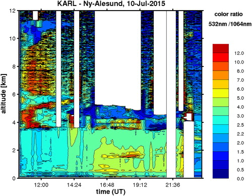
The BB event started over our site on 9 July 2015, but measurements with KARL were available first on 10 July. Air temperature was around +10 °C at 2 m above ground, and the surface was free of snow and ice. Fig. 1 gives an overview of the vertical aerosol backscatter coefficient on that day (similar to Markowicz et al., 2016). White stripes indicate excluded data due to multiple scattering in the figure. Only the structures around 12 UTC in 10–12 km altitude and between 14 and 22 UTC at about 5 km altitude are clouds. This can be seen from the colour ratio in Fig. 2 which shows small values (large particles) for the clouds. All other features are BB aerosol. This aerosol occurs mainly below 4 km altitude in distinct structures and shows backscatter coefficients of more than 10 Mm⁻¹sr⁻¹ for λ = 532 nm. A clear transition between very polluted and relative clean air masses below 4 km altitude before noon can be clearly seen. Details on the origin of the event and its distribution in time are described in Markowicz et al. (2016).

Fig. 1. Aerosol backscatter coefficient on 10 July 2015 as recorded by the KARL lidar at 532 nm (colour-coded). White stripes indicate excluded data due to multiple scattering.

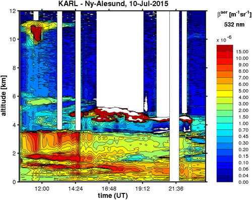
Fig. 2. Colour ratio derived from the wavelengths of 532 nm and 1064 nm as a rough indicator of the particles’ size.

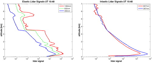
Exemplarily some lidar profiles for the time of the radiosonde launch (UT 10:48) are shown in Fig. 3. The clear, abrupt transition between very polluted and quite clear conditions at about 3.5 km altitude is again evident. Due to the high extinction coefficients of the event a retrieval of the extinction coefficients from the Raman shifted wavelengths was possible up to that altitude.

Fig. 3. Exemplary lidar profiles in for the elastic (left) and inelastic scattering (right) for the time UT 11:48, contemporary to the radiosonde.

The (volumetric) backscatter and extinction coefficients derived from the lidar data for the time of the launch of the radiosonde are presented in Fig. 4. Again, the sharp transition between polluted and clean conditions in about 3.5 km altitude is evident. Moreover, a layered structure below about 2.1 km altitude is visible, while above that no more layers but rising values with altitude are found.

Fig. 4. Profiles of the aerosol backscatter coefficient (left) and the aerosol extinction coefficient (right) for the time of the launch of the radiosonde.

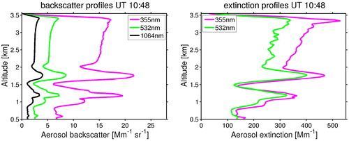
Generally, the backscatter and extinction coefficients are extremely high for the European Arctic. Ritter et al. (2016) derived for 355 nm typical aerosol extinction coefficients around 20 Mm⁻¹ for the generally more polluted spring time in about 2 km altitude. Hence, this event increased the backscatter and extinction coefficients roughly by a factor of 20. This extreme air pollution allowed a detailed analysis of the lidar data. It can be also estimated from Fig. 4 that the noise in the extinction coefficient at 532 nm (the weakest channel), is around 20 Mm⁻¹ in 3 km altitude and hence the error is below 10%, which is required for the derivation of aerosol microphysics from lidar data (Veselovskii et al., 2002).

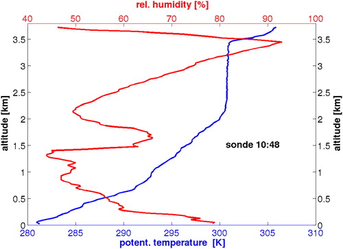
The profiles of potential temperature and relative humidity (RH) over water from the radiosonde measurements are given in Fig. 5. The altitude of the (elevated) temperature inversion in about 3.5 km coincides precisely with the top of the aerosol plume in Fig. 4, revealing how this inversion effectively traps the aerosol and inhibits most vertical exchange. Moreover, several moist layers were present up to 10 km altitude above the range shown in Fig. 5. The aerosol rich altitudes between 2.1 km and 3.5 km altitude are characterised by an almost neutral potential temperature gradient, while the RH increases from about 50% to 90% giving an excellent opportunity to study any hygroscopic effects of the aerosol. The local boundary layer was very low, about 100 m altitude, see blue curve in Fig. 4 and Markowicz et al. (2016).

Fig. 5. Radiosonde profiles on 10 July 2015 of potential temperature (blue) and relative humidity over water (red) from a RS-92 sonde on 10 July, 2015.

3. Description of the mathematical inversion scheme

3.1. Mathematical preliminaries for the inversion

In this section, it is described how aerosol microphysical properties are derived from lidar data. The model relating the optical parameters Γ(λ) with the volume size distribution v(r) is described by a Fredholm integral operator T of the 1st kind (4) $$\left(\text{Tv}\right)\left(\lambda \right)={\int }_{r_{\text{min}}}^{r_{\text{max}}}K\left(r,\lambda ;m\right)v\left(r\right)\mathrm{d}r={\int }_{r_{\text{min}}}^{r_{\text{max}}}\frac{3}{4r}Q\left(r,\lambda ;m\right)v\left(r\right)\mathrm{d}r=\Gamma \left(\lambda \right),$$(4) where λ is the wavelength, r is the radius, m is the complex refractive index, Γ(λ) denotes either the extinction or backscatter coefficients, K is a kernel function and Q stands for either the extinction or the backscatter (dimensionless) Mie efficiencies respectively, i.e. the particle cross sections divided by the geometrical cross section of a sphere. The integral limits r_min and r_max are appropriate lower and upper radii which are describing the specific measurement event but have also to respect the restriction of the physical model. Therefore, here for the lower limit 0.001 µm and for the upper one 2 µm were used. This upper limit was chosen, because sometimes in the calculations a mode in the transition between fine and coarse around 1 µm has been found, hence our chosen upper limit includes this mode without extending the calculation interval too much. We will call this mode in the transition region ‘coarse mode’ later for simplicity.

As the input data is provided by the KARL lidar, 5 discrete values of input data can be provided: the 3 backscatter coefficients at 355 nm, 532 nm and 1064 nm and 2 extinction coefficients at the former 2 wavelengths.

Identifying Γ(λ) as our measurement data and v(r) as the unknown distribution, the problem reduces to the inversion of the operator T. Knowing the volume size distribution, we can then extract the following microphysical parameters:

• total surface-area concentration s_t = 3$\int \frac{v(r)}{r}\mathrm{d}r$ (µm² cm⁻³)

• total volume concentration v_t =$\int v\left(r\right)\mathrm{d}r$ (µm³ cm⁻³)

• effective radius r_eff = 3 v_t/a_t (µm)

• total number concentration n_t = $\frac{3}{4\pi }\int \frac{v(r)}{r^3}\mathrm{d}r$ (cm⁻³).

In addition, the complex refractive index m = m_R + i m_I with the real part Re(m) = m_R and imaginary part Im(m) = m_I as well as the single scattering albedo (SSA) in 355 nm and 532 nm are retrieved. Note that in this work the common assumption of wavelength independent refractive index is made, as a member of the predefined grid introduced see Fig. 6. In detail, the determination of the refractive index is not uniquely. All possible refractive indices are lying on a ‘diagonal’ pattern. Selecting the best points on the diagonal with respect to least residual error and with similar volume size distribution results in a mean refractive index, which is used to calculate a mean SSA as usual. Solving the above integral equation requires discretization, regularisation and a parameter choice rule, see e.g. Böckmann et al. (2005), Samaras et al. (2015) and Müller et al. (2016).

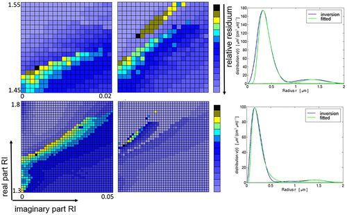
Fig. 6. First row: Inversion results for layer 2 (1717–1777 m). Left, centre, right: (20 × 20)-grid of refractive index RI at 10:48 UTC, (20 × 20)-grid of RI at 12:07 UTC, retrieved volume distribution at 10:48 UTC. Second row: Inversion results for layer 3 (2166–2436 m). Left, centre, right: (40 × 40)-grid of RI at 10:48 UTC, (40 × 40)-grid of RI at 12:07 UTC, retrieved volume distribution at 12:07 UTC.

In order to solve the Fredholm equation, a grid (Fig. 6) of viable options for the refractive index, i.e. all combinations of real parts and imaginary parts of the refractive index |Re(m)| x |Im(m)| is assumed otherwise we have to deal with a non-linear problem. We discretized the Fredholm equation with spline collocation, a method well suited for our case since the optical data are only given in specific wavelengths and additionally it reduces the computational effort. The volume size distribution v(r) is approximated with respect to the B-spline functions Φ_j by $v_n={\sum }_{j=1}^n{b}_j{\Phi }_j$, reducing the problem to the determination of the coefficients b_j. B-spline functions, polynomials of degree d-1 with compact support, are very favorable with respect to low numerical effort. The continuous integral problem is now replaced by a discrete one Ab = Γ, where the matrix elements of the linear system are (5) $$A_{ij}={\int }_{r_{\text{min}}}^{r_{\text{max}}}K({\lambda }_i,r;m){\Phi }_j\left(r\right)\mathrm{d}r.$$(5)

By doing so, we have already projected our problem to a finite n-dimensional space. Clearly, the decision about the projected dimension n and the order d, degree of polynomials plus one, of the base functions Φ_j is critical, since an appropriate representation of our solution strongly depends on it. This is not done at once; on the contrary, the algorithm constructs a linear system (5 × n) for each value of n and d specified and every refractive index within our predefined grid. For example, we first fix the refractive index and calculate the kernel functions, then decide for candidates of n and d, e.g. n = 5, …, 8 and d = 3,4 which define a B-spline function and finally calculate the matrix elements A_ij. For more particular details on the B-spline basis in the frame of a non-negative size distribution we are looking for, see Böckmann (2001).

Each linear system is solved by first expanding the matrix using Singular Value Decomposition (SVD). Potential noise in our matrix will be magnified as a result of the singular values clustering to zero. We would like to prevent this behavior by including only a part of the SVD, i.e. defining a certain cut-off level k, below which the noisiest solution coefficients are filtered out. This regularisation procedure is known as the Truncated SVD (TSVD), see Böckmann (2001). The parameter choice rule consists of selecting an appropriate triple (n,d,k) heuristically.

It is now clear that the solution space created by our algorithm is quite huge consisting of |n| x |d |x |k| x |Re(m)| x |Im(m)| solutions overall, where |.| denotes the amount of different values of the specific parameter. The solution space is restricted in the following way: For every specific refractive index, the best triple (n, d, k) is picked in terms of least residual error (forward calculation with v(r) and comparing the difference of received and measured coefficients), and the resulting solution grid is presented with a log-colour scale relevant to the error magnitude. This visual representation is very convenient for the post-processing procedure. At this point we are able to screen 3 solution spaces with respect to different error types (so called mathematical measures or norms, respectively): the 2- Euclidian norm of (i) the absolute or (ii) the relative error and (iii) the maximum norm of the relative error. We end up using both relative types of the error measure, i.e. (ii) and (iii). Finally, only a few solutions (10–25) are averaged to produce the mean microphysical properties and a deviation bar from the mean is given, Samaras et al. (2015).

The retrieval by TSVD was first done with a refractive index grid with a resolution of 40x40 points and a range for the Re(m) from 1.3 to 1.8 and for the Im(m) from 0 to 0.05, see Fig. 6 (second row). We found that the best possible refractive indices lay on a diagonal pattern what is an indication of precise measurements in agreement with investigated simulations, see Müller et al. (2016). The best points are situated in a particular range (cluster) for the real and imaginary part. Therefore, the retrieval was done a second time on those ranges with a grid resolution of 20x20 points, see Fig. 6 (first row). As already mentioned before, the best points are lying in a connected cluster with quite the same retrieved volume size distribution and with least residual error with respect to one selected norm. This approach was already used successfully for other measurements events see, e.g. Hoffmann et al. (2012), Samaras et al. (2015) and Ortiz-Amezcua et al. (2017).

We explicitly indicate that the inverted function shape (curve) of the volume distribution is free during the retrieval procedure, i.e. no previous restriction is used. In spite of this fact, very often a log-normal shape of the volume distribution (mono-, bi- or multimodal, respectively) was found. Therefore, the commonly assumed log-normal shape seems to be often true, i.e. the number distribution is a log-normal distribution, too. This property is also true for the surface-area distribution. All three distribution types have the same geometric standard deviation (gsd). Therefore, if the retrieved volume distribution is a bimodal one similarly to two log-normal shapes, we separated the inverted distribution by fits into two modes (fine and coarse mode) by using two log-normal distribution shapes such that the sum of both modes fits the retrieved volume distribution well, see Fig. 6, on the right. Finally, we determined all microphysical parameters for the complete retrieved volume distribution as well as for the two modes separately.

3.2. Selection of measurement times and appropriate particle layers

The inversion of the microphysical aerosol properties was done at two different times: at 10:48 UTC (contemporaneous to the radiosonde for valid humidity measurements) and at 12:07 UTC to evaluate if the selected aerosol particle layers are stable or not. We note that other remote sensing devices at the site do not see any changes in the meteorological conditions between 11 and 12 UTC. Five layers were selected for the derivation to some particular rules.

The main criterion was to find layers with different relative humidity (RH) and otherwise homogeneous intensive quantities, as lidar ratio, colour ratio and Ångström exponent to infer how the aerosol microphysical properties are changing with humidity.

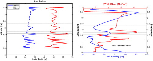
The first layer 1 was selected from 1537 to 1597 m altitude with thickness 60 m and humidity of 62–65% and quite high lidar ratios of 30.5 sr and 65 sr for 355 nm and 532 nm, respectively. The second layer 2 is in the altitude range 1717 to 1777 m, with similar relative humidity of 64–65%, high values of backscatter but lower lidar ratios (21.5 sr and 47 sr). The third layer 3 has the lowest RH of 50–55% and is vertically most extended (270 m) ranging from 2166 to 2436 m. The fourth layer 4 is 120 m thick with a RH of 80–85%, in the altitude range 3186–3306 m. The highest layer 5 has the largest RH of 90–92% and ranges from 3366 to 3426 m. The selected layers are shown in Fig. 7. Overall the LR(532 nm) values are in agreement with Müller et al. (2007b) for Arctic haze and Canadian forest fire smoke.

Fig. 7. Selection of the layers (vertical dotted lines) in terms of the lidar ratios (left), RH and aerosol backscatter coefficient (right) (Data for 10:48 UTC).

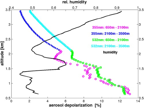
The lowest layer 1 has the largest depolarisation ratio 8–10% for 355 and 532 nm, therefore it is not sure if the spherical particle model may be assumed. Nevertheless, we inverted the layer with the spherical model. It is an ongoing work to evaluate the layer within a spheroidal model, see Böckmann and Osterloh (2014). For this reason, we could not invert data below 1500 m altitude here. All other layers have depolarisation ratios well below 6% for 355 and 532 nm (except layer 3 for 532 nm on average 7.4%) and the spherical model may be assumed, see Fig. 8. Moreover, in layer 4 and 5 the humidity is 84 and 91%. The particles may take up more water and should be, therefore, more spherical which correlates with the decreasing depolarisation.

Fig. 8. Aerosol depolarisation at 355 nm and 532 nm and relative humidity (black line) for comparison.

4. Results

4.1. Optical properties derived by lidar

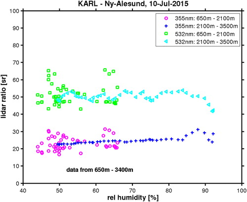
In this section the hygroscopicity of the aerosol is studied. For this purpose, the lidar ratio (LR), the colour ratio (CR) and the depolarisation (δ) are given as functions of the relative humidity for the launch time of the radiosonde (one profile averaged from 10:48 till 10:59).

First, the LR at λ = 355 nm and 532 nm is again given in Fig. 9, now as a function of relative humidity. We divided the profile in two intervals: below and above 2.1 km, and found generally more homogeneous particle properties above. This coincides to the atmospheric stability described by the potential temperature profile in Fig. 5, with stable conditions below and neutral conditions above 2.1 km altitude. The LRs for both wavelengths are similar to values found by Ritter et al. (2016) for Arctic Haze. Interestingly, no clear change of LR with increasing humidity can be seen. A possible uptake of water by BB aerosol should decrease the refractive index and increase the particle size. Probably also the shape may become more spherical if the aerosol takes up some water. All these effects should influence the LR. For example, Ackermann (1998) estimated the dependence of LR on humidity also using Mie theory and prescribed aerosol properties (dry radii and refractive index) and found an increase of LR in more moist conditions for soluble aerosol. However, the LR seems to be considerably independent from the relative humidity in our study, resembling more the ‘desert aerosol’ case of Ackermann (1998).

Fig. 9. The lidar ratio as function of the relative humidity for lidar data contemporary to the radiosonde (10:48 – 10:59 UTC).

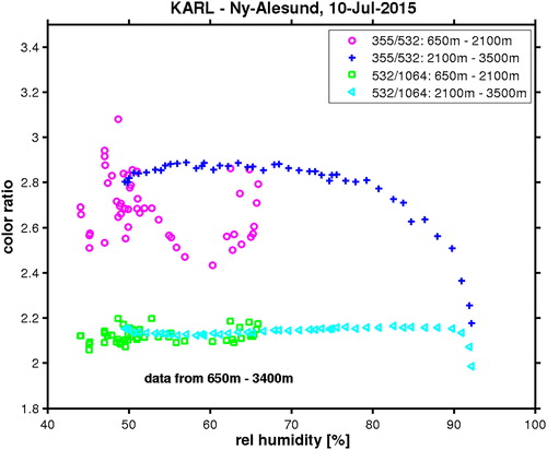
In Fig. 10 in a similar fashion the colour ratio is plotted as a function of relative humidity. ‘355/532’ refers to the CR of these two wavelengths, while ‘532/1064’ refers to the colour ratio of the longer wavelengths, which is more sensitive to the larger particles. (The reason for this is that in the scattering efficiency the size parameter, particle circumference divided by wavelength, is decisive, e.g. van de Hulst, 1981). So, from Fig. 10 it is evident that the larger particles which are best visible in the 532/1064 CR are non-hygroscopic up to 90% relative humidity, while the smaller particles, which are best visible in the 355/532 CR, show a slightly increased variability in the lowest 2.1 km of the atmosphere and seem to increase in diameter at about 80% RH. Overall, however, the aerosol seems more hygrophobic than the common Arctic aerosol species as sulphate and sea salt, which start to increase their diameter by water uptake already at humidities of RH >55% (Zieger et al., 2010, 2011).

Fig. 10. Colour ratios in 355/532 and 532/1064 as function of the relative humidity for lidar data contemporaneous to the radiosonde.

It is difficult to judge to what extent the depolarisation is influenced by the relative humidity, as δ decreases strongly with altitude (Fig. 8, previous section). The small decrease of δ in around 1.85 km altitude is probably not correlated to a local maximum in RH as this occurs already 200 m lower with only 67%. Above 2 km altitude, in the region of increasing RH the depolarisation drops moderately from slightly over 6% to 3% for 532 nm. Hence it seems as if the particles become slightly more spherical in a moister environment, but as particle growth is only evident at RH >80% (which is above 3.15 km altitude where δ < 2.8%) the overall conclusion is that the BB aerosol is generally hydrophobic and we only expect above 80% RH for the layers 4 and 5 a change in the microphysical properties (change from ‘dry’ to ‘wet’).

4.2. Inversion of lidar data

All five above defined layers were inverted with respect to data at t1 = 10:48 and t2 = 12:07 UTC. Relative humidity data are additionally available, as already mentioned before, for the earlier time. All microphysical retrievals are given in Tables 1 and 2. During the time span between t1 and t2, layer 2 was most stable (Tables 1 and 2 and Fig. 11 right side). Moreover, Fig. 11 (right side) also shows that layers 3 and 4 were also quite stable. In layer 3 mostly the refractive index is varying but still within a range that is about the uncertainty in its retrieval (about 0.02 in the real and 0.005 in the imaginary part, see Fig. 6), whereas in layer 4 the total surface-area concentration varies most.

Fig. 11. First row: Comparison of effective radii. Left: Effective radii (fine, fine+coarse and complete inverted) for the five investigated layers with different relative humidity at 10:48 UTC, showing the hygroscopic growth. Right: Comparison of the inverted effective radius and surface-area concentration for the five layers at two different times: 10:48 UTC and 12:07 UTC, showing the stability of the parameters. Second row: Comparison of the real and imaginary part of the refractive index. The error bar represent the standard deviation from the mean value.

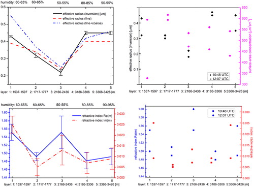
Fig. 12. Retrieved volume distribution and log-normal fits for fine and coarse mode.

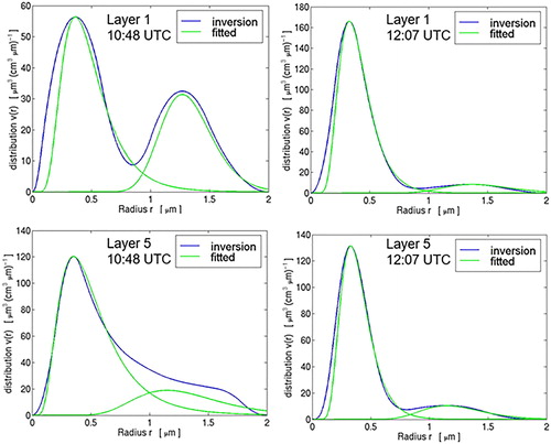
Fig. 13. Integrated aerosol extinction in a layer [1500 m …. 3500 m] from the lidar (black diamonds) and photometer AOD for that interval for different assumptions on cloud contamination.

Fig. 14. Size distribution for the whole evaluable layer from 1500 m to 3500 m altitude, above: only lidar (3 backscatter and two extinction coefficients), below: lidar and photometer, hence in total same 3 backscatter and 2 + 9 extinction coefficients.

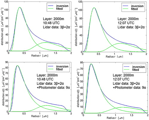
Fig. 15. Comparison between (incoming) radiation components: direct and diffuse solar and longwave downward radiation for the BB event (10 July, 2015) and a clear background day (10 July, 2016).

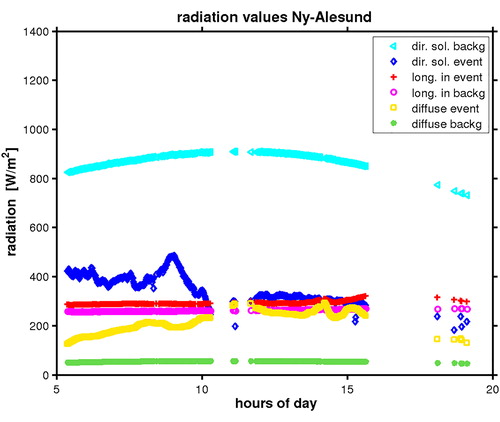
Table 1. This table collects all microphysical properties for the first measurement time at 10:48 UTC.

Altitude [m], thickness [m] (10:48UTC)	RH [%] mean RH [%] LR: sr] 355/532	RI Re(m)	RI Im(m)	Effective radius [µm]	Median radius (gsd) [µm]	Total surf.-area concentr. [µm^2/cm^3]	Total volume concentr. [µm^3/cm^3]	Total number concentr. [1/cm^3]	SSA(355)	SSA(532)
1537–1597 60 [fine/coarse]	62–65 64 30.5/65	1.55 ± 0.02	0.025 ± 0.004	0.43 ± 0.004 0.39/1.28	0.24(1.56)/ 1.2(1.18)	329 ± 4.1 189 /39.5	47.5 ± 0.33 25.3/16.9	168/2.1	0.781 ± 0.004	0.823 ± 0.003
1717–1777 60 [fine/coarse]	64–65 65 21.5/47	1.49 ± 0.01	0.005 ± 0.004	0.32 ± 0.013 0.34/1.40	0.25(1.42)/ 1.3(1.19)	617 ± 5.9 456/13	65.7 ± 2.99 52.3/5.7	440/0.6	0.955 ± 0.007	0.970 ± 0.003
2166–2436 270 [fine/coarse]	50–55 53 23/50.5	1.55 ± 0.04	0.013 ± 0.007	0.22 ± 0.0172 0.24/1.36	0.12(1.7)/ 1.3(1.14)	534 ± 30.7 398/5.6	39.4 ± 2.44 31.6/2.5	1245/0.3	0.914 ± 0.037	0.930 ± 0.026
3186–3306 120 [fine/coarse]	80–85 84 26.6/52.6	1.48 ± 0.02	0.007 ± 0.005	0.45 ± 0.01 0.40/1.63	0.19(1.71)/ 1.60(1.08)	561 ± 2.5 501/11.2	83.7 ± 2.24 66.3/6.1	602/0.35	0.919 ± 0.030	0.942 ± 0.017
3366–3426 60 [fine/coarse]	90–92 91 26/45.5	1.49 ± 0.02	0.009 ± 0.005	0.45 ± 0.01 0.40/1.20	0.20(1.69)/ 0.96(1.35)	543 ± 2.8 477/41	82.0 ± 2.80 64.2/16	534/3	0.898 ± 0.066	0.927 ± 0.037
mean value		1.51	0.0118	0.374		516.8	63.72		0.893	0.918
1500–3500 2000 [fine/coarse]		1.50 ± 0.03	0.010 ± 0.006	0.46 ± 0.014 0.41/1.23	0.23(1.61)/ 0.97(1.36)	464 ± 3.2 379/46	71.8 ± 2.5 50.8/18.3	367/3.4	0.888 ± 0.068	0.920 ± 0.038
Lidar + Photom 1500–3500 [fine/coarse]		1.58 ± 0.04	0.009 ± 0.005	0.44 ± 0.02 0.36/1.26	0.14(1.84)/ 1.04(1.32)	363 ± 4.0 383/22.3	52.8 ± 2.1 44.0/9.2	769/1.5	0.899 ± 0.065	0.920 ± 0.041

Remark: [fine/coarse] is only valid for columns 5–9. The values v_t and a_t refer to the inverted total distribution (the blue curves in Figures 12 and 14, not to the sum of the log-normal fits).

Table 2. This Table collects all microphysical properties for the second measurement time at 12:07UTC.

Altitude [m] thickness [m] (12:07UTC)	RI Re(m)	RI Im(m)	Effective radius [µm]	median radius (gsd) [µm]	total surf.-area concentr. [µm^2/cm^3]	total volume concentr. [µm^3 /cm^3]	total number conentr[cm^–3].	SSA(355)	SSA(532)
1537–1597 60 fine/coarse	1.5 ± 0.01	0.004 ± 0.003	0.32 ± 0.011 0.35/1.39	0.25(1.45)/ 1.26(1.22)	595 ± 4.3 362/12	64.2 ± 2.3 54.2/5.6	449/0.6	0.964 ± 0.006	0.976 ± 0.003
1717–1777 60 fine/coarse	1.51 ± 0.02	0.006 ± 0.003	0.30 ± 0.011 0.33/1.17	0.26(1.37)/ 0.87(1.41)	594 ± 6.4 414/21	60.3 ± 2.74 45.3/7.8	413/2	0.946 ± 0.019	0.963 ± 0.009
2166–2436 270 fine/coarse	1.6 ± 0.02	0.007 ± 0.002	0.18 ± 0.006 0.19/1.42	0.10(1.65)/ 1.35(1.15)	473 ± 31.2 374/3.8	27.8 ± 1.12 23.8/1.8	1735/0.2	0.957 ± 0.002	0.964 ± 0.002
3186–3306 120 fine/coarse	1.50 ± 0.02	0.009 ± 0.006	0.47 ± 0.02 0.41/1.23	0.22(1.64)/ 0.83(1.49)	460 ± 2.9 377/52	70.0 ± 3.36 50.6/19.6	386/5	0.896 ± 0.091	0.926 ± 0.051
3366–3426 60 fine/coarse	1.56 ± 0.05	0.024 ± 0.010	0.35 ± 0.02 0.35/1.18	0.26(1.42)/ 1.04(1.25)	431 ± 1.9 345/17	50.4 ± 2.89 40.2/6.7	326/1.1	0.812 ± 0.019	0.871 ± 0.010
mean value	1.53	0.0100	0.324		514.6	54.54		0.915	0.940
1500–3500 2000 fine/coarse	1.50 ± 0.03	0.010 ± 0.007	0.47 ± 0.019 0.41/1.23	0.23(1.62)/ 0.97(1.36)	464 ± 3.8 382/46	72.0 ± 3.2 51.4/18.2	374/3.3	0.885 ± 0.082	0.918 ± 0.046
Lidar + Photom. 1500–3500 fine/coarse	1.66 ± 0.05	0.015 ± 0.004	0.37 ± 0.02 0.30/1.31	0.10(1.94)/ 0.94(1.44)	382 ± 3.0 388/23	47.3 ± 2.2 39.1/9.2	1248/1.8	0.859 ± 0.065	0.894 ± 0.016

Remark: [fine/coarse] is only valid for columns 4–8. The values v_t and a_t refer to the inverted total distribution (the blue curves in Figures 12 and 14, not to the sum of the log-normal fits).

The layers 1 and 5 are instable during this time frame. Therefore, we concentrate in more detail on the evaluation of layers 2–4.

Only briefly, at 10:48 UTC layer 1 shows a bimodal distribution which disappears more or less completely at 12:07 UTC, see Fig. 12 (first row). This variability in the size distribution might be a consequence of a decreasing lidar ratio (from 65 sr/30 sr for 355 nm and 532 nm respectively at 10:48 UTC to 42 sr/20 sr at 12:07 UTC). Hence this altitude interval may not belong to the same layer. Moreover, we cannot rule out an artefact due to the high depolarisation. Nevertheless, using Mie theory the easiest way to explain the relative high lidar ratios at 10:48 UTC is by the assumption of a second (larger) mode in the size distribution.

Layer 5 behaves similar to layer 1 but less pronounced. The second mode is smaller as before; see Fig. 12 (second row). For layer 5 the lidar ratios hardly change; for both times we got 45 sr at 355 nm and 25 sr for 532 nm.

Layer 4 was already investigated in detail by Böckmann et al. (2017); therefore, we give only the retrieved microphysical properties in Tables 1 and 2.

Next, we are going to evaluate the stable layers 2 and 3 in detail, see Fig. 6, previous section. The refractive index grids show prominent diagonals for both layers and times. Concerning layer 2 for both times the second (20 × 20)-grids, i.e. restricted in terms of ranges for real and imaginary parts of m are given whereas for layer 3 the first (40  × 40)-grids are presented. The first grids show much better the thin diagonals. The diagonal pattern indicates a stable inversion procedure in line with our expertise in simulation studies. All four refractive index grids in Fig. 6 present the maximum norm of the relative forward error. The volume distributions for both layers are changing only a little bit during the time segments, therefore, only one graph per layer is given in Fig. 6.

Both volume distributions have two modes a fine and a coarse mode although the coarse mode is only weakly pronounced.

Evaluating the hygroscopic growth at 10:48 UTC we found for the layers 2–5 the following effective radii: 0.32, 0.22, 0.45, 0.45 µm, see also Fig. 11 (first row, left side). This correlates with the RH (65, 53, 84 and 91%) as well as with the particle linear depolarisation ratio (5.8, 2.6 and 2.3) for layers 3–5. As one notices the radius does not increase further from layer 4 to 5. However, the effective radius (fine + coarse) shows the hygroscopic growth with respect to layers 2–5 most obviously (0.37 µm, 0.25 µm, 0.42 µm, 0.46 µm). Moreover, the colour ratio for layers 2–5 (2.55, 2.85, 2.69 and 2.38) is also quite good in agreement with the hygroscopic growth of the effective radii except for layer 4 where the value is too big.

The hygroscopic growth is confirmed by the refractive index; see again Fig. 11 (left side, second row). The mean real parts of m for layers 2–4 are 1.49, 1.55 and 1.48 which is in agreement with the RH and points out that the particles take up water. The imaginary part of m has always the largest uncertainties during the retrieval procedure, see Müller et al. (2016). The error bars are large (standard deviation of all selected values from the mean value). The mean imaginary parts of m for layers 2–4 are 0.005, 0.013 and 0.007, respectively. This is still in agreement with the RH under consideration of the deviation bars.

4.3. Inversion results including the photometer data

To obtain overall height averaged aerosol properties and to check for consistency we included the AOD of the 9 aerosol devoted wavelengths from the photometer in the inversion software. For this, we averaged the lidar data in the interval [1500 m … 3500 m], which is the complete height interval in which Mie theory should be a valid assumption and thick BB aerosol is present. Next, we estimated from the lidar, which fraction of the extinction should be located in this interval. As in the Arctic the sun-photometer and the lidar (close to zenith) do not point into the same direction the sporadic existence of the high cirrus in 11 km at 12 UTC in Fig. 1 introduced some uncertainty, see Fig. 13. If the photometer had not seen any cirrus the AOD fraction in the interval of interest would have been too high (and vice versa, see Fig. 13). Thus, we could estimate the probable cloud contamination in the photometer that matches to the lidar.

Two more inversions of the aerosol microphysics have been performed. First, we only used lidar data (case 1) for the whole layer of 2000 m from 1500 to 3500 m altitude. Second, we evaluated jointly lidar and photometer data (case 2), see Tables 1 and 2 last two rows for the column microphysical properties and Fig. 14 for the volume distributions.

With respect to case 1 we found: Although the layers 1 and 5 were variable during the two measurement times, the whole column (2000 m) is stable, see the volume distributions in Fig. 14 (first row). The microphysical parameters for 10:48 and 12:07 UTC (in brackets) are: m_R=1.5 (1.5), m_I = 0.01 (0.01), r_eff = 0.46 (0.47)µm, s_t = 464 (464) µm²/cm³, v_t = 71.8 (72.0)µm³/cm³, n_t (fine mode) = 367 (374) cm⁻³ and n_t (coarse mode) = 3.4 (3.3) cm⁻³. This is actually noteworthy and shows the stability of the retrieval procedure during stable meteorology conditions with respect to this event.

Concerning case 2 with respect to the two time frames the volume distributions look in principle qualitatively stable, see Fig. 14 (second row). The microphysical parameters deviate more or less for the complete inverted volume distribution, see Tables 1 and 2. However, comparing the fits of fine and coarse mode in detail this results in tolerable values. For the fine mode it yields: r_eff = 0.36 (0.30) µm, s_t = 383 (388) µm²/cm³, v_t = 44.0 (39.1) µm³/cm³, n_t = 769 (1248) cm⁻³. For the coarse mode we found: r_eff = 1.26 (1.44) µm, s_t = 22.3 (23.0) µm²/cm³, v_t = 9.2 (9.2) µm³/cm³, n_t = 1.5 (1.8) cm⁻³. For the fine mode, the determination of the total number concentration is always a challenge since very small particles have a huge effect on it.

The information content of the sun photometer data matches more or less to both lidar measurement times with respect to the effective radius, total surface-area and volume concentration. But the retrieval of the refractive index is different at both times and it seems to fit better to 10:48 UTC.

It is also interesting to compare the results for the cases 1 and 2 at 10:48 UTC. Having in mind the different viewing direction of the photometer the following results are acceptable comparing case 1 and 2: m_R = 1.5 (1.58), m_I = 0.01 (0.009), r_eff = 0.46 (0.44)µm, s_t = 464 (363) µm²/cm³, v_t = 71.8 (52.8)µm³/cm³, n_t (fine mode) = 367 (769) cm⁻³ and n_t (coarse mode) = 3.4 (1.5) cm⁻³.

Finally, we are going to compare the SSA. In face of the microphysical properties within tolerable limits for cases 1 and 2 the SSA is in a good shape. We found for case 1(10:48 UTC), case 1(12:07 UTC) and case 2(10:48 UTC): SSA (355 nm) = 0.888, 0.885 and 0.899 or SSA(532 nm) = 0.920, 0.918 and 0.920, respectively. This result is remarkable as it shows some constant absorbing fraction within the aerosol layer without evident uncertainty of the inversion process.

4.4. Radiative impact

In this section we follow ideas of Bush and Valero (2003) or Markowicz et al. (2008) and analyse the radiative impact, both the aerosol radiative forcing and the aerosol modification factor AMF of the BB event in dependence on the AOD. This radiative impact can easily be seen by comparing the surface radiation values for the event day (10 July, 2015) with a clear air background day (10 July, 2016). Due to the fact that 2016 was a leap year there are slight differences between the event and background day in solar declination (< 0.25°) and solar culmination (< 1 minute). The difference in solar declination has been neglected. Also, we neglect the slightly higher humidity on the event day (3.5 cm water column, compared to 1.5 cm on the background day, retrieved from radiosonde profiles, respectively). In Fig. 15, the normalised direct and diffuse solar radiation as well as the downward longwave radiation is shown. For the calculation of the aerosol radiative forcing and the AMF, all data points have been considered for which (a) the AOD of the event was larger than 0.5 at 500 nm, (b) the AOD of the background was smaller than 0.05 at 500 nm, (c) the Angström exponent (as a fit through all sun photometer AOD values) of the event was smaller than –1.4 (meaning that AOD is proportional to λ^−1.4, hence no cloud contamination of the event day) and (d) the difference in the net longwave flux between event and background day was smaller than 25 W/m². These four conditions guarantee that the background is neither aerosol nor cloud influenced and that data from the event day does not contain cloud contamination. It can be seen that the BB event reduces the direct radiation strongly by roughly a factor of 2. Part of this is compensated however by an increase of diffuse radiation. Also, the longwave downward radiation is increased slightly by about 20%. Such a behaviour is expected as the aerosol blocks or scatters part of the (incoming) downward solar radiation and also reflects some of the upward terrestrial longwave radiation back to the surface.

In this work, we define the aerosol radiative forcing ΔF as the difference in net total radiation fluxes F between disturbed (aerosol event) and undisturbed (clear air background) for perpendicular incidence on the surface: (6) $$\Delta F=\mathrm{ }{F}_{\text{net}}^{\text{aer}}-\mathrm{ }{F}_{\text{net}}^{\text{backg}}\mathrm{ }$$(6)

with (7) $$F_{\text{net}}^{}=\mathrm{ }{F}_{}^{\downarrow }-\mathrm{ }{F}_{\mathrm{ }}^{\uparrow }=\mathrm{ }{F}_{\text{SW}}^{\downarrow }-\mathrm{ }{F}_{\text{SW}}^{\uparrow }+\mathrm{ }{F}_{\text{LW}}^{\downarrow }-\mathrm{ }{F}_{\text{LW}}^{\uparrow }\mathrm{ }$$(7) where SW and LW represent the broad shortwave (200 nm to 3600 nm) and longwave (4 µm to 50 µm) radiation, and the arrows ↑ upward (outgoing) and ↓ downward (incoming) radiation, respectively.

Further, we define (similar to the cloud modification factor) an aerosol modification factor AMF as the ratio of polluted versus clear irradiances on a horizontal plane: (8) $${\text{AMF}}_{\text{SW}}=\mathrm{ }\frac{F_{\text{global}}^{\text{aer}}}{F_{\text{global}}^{\text{backg}}}\mathrm{ }$$(8)

However, the downward longwave radiation strongly depends on the upward longwave radiation which itself is a function of the surface temperature. Hence, aerosol (or cloud) radiative effects become better understandable if the net longwave radiation for the aerosol and background case is considered. Thus, we define: (9) $${\text{AMF}}_{\text{LW}}=\mathrm{ }\frac{F_{\mathrm{L}\mathrm{W},\downarrow }^{\text{aer}}-\mathrm{ }{F}_{\mathrm{L}\mathrm{W},\uparrow }^{\text{aer}}\mathrm{ }}{F_{\mathrm{L}\mathrm{W},\downarrow }^{\text{backg}}-\mathrm{ }{F}_{\mathrm{L}\mathrm{W},\uparrow }^{\text{backg}}\mathrm{ }}\mathrm{ }$$(9)

The results are given in the Figs. 16–18. First in Fig. 16 the shortwave AMF is given as a function of AOD for the BB aerosol event. A non-linear decrease with AOD can be seen. For an AOD (at 500 nm) of 1 the global radiation drops to about 74% of the clear sky case. For low solar altitudes even less radiation reaches the surface and the radiative impact seems to be higher, hence only solar elevations >25̊ above the horizon have been considered. To understand this behaviour we chose an approach which considers an exponential decrease simply from the Lambert’s law and a brightening due to multiple scattering, as the photometer’s AOD with its small field of view of 1̊ hardly is affected by multiple scattering. This is clearly different for the hemispheric radiation as can be seen in the increase of the diffuse radiation in Fig. 15. Therefore we write: (10) $${\text{AMF}}_{\text{SW}}=\exp \left(-\mathrm{ }\gamma \mathrm{ }·\text{AOD}\right)·\left(1+c\mathrm{ }·\mathrm{ }{\text{AOD}}^2\right)\mathrm{ }$$(10)

Where γ translates the effective spectral sensitivity of the shortwave Kipp & Zonen sensors to the AOD at 500 nm, and c describes the effectivity of the multiple scattering. We found γ = 0.35 and c = 0.05. This fit is given by the solid black line in Fig. 16. The dotted line artificially sets c = 0 and hence neglects any multiple scattering.

The longwave AMF is given in Fig. 17. Here the radiative impact is overall lower, as the AOD decreases with wavelength (Markowicz et al., 2016). Lower solar elevations result in less incoming radiation, so again only solar elevation >25̊ have been used and with the same approach as before we derive (11) $${\text{AMF}}_{LW}=\exp \left(-\mathrm{ }0.22\mathrm{ }·\text{AOD}\right)·\left(1+0.07\mathrm{ }·\mathrm{ }{\text{AOD}}^2\right)\mathrm{ }$$(11)

So effectively in the infra-red the optical thickness of the aerosol plume is only 22% of the AOD at 500 nm and the multiple scattering seems to be slightly higher than before.

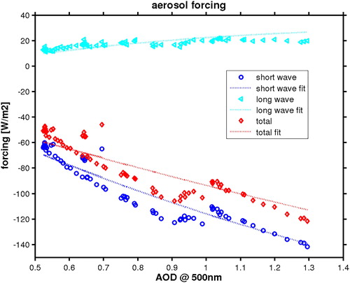
In Fig. 18, the aerosol forcing is given, both from the observations (thick bullets, dots and diamonds) as well as from the fits of the AMF for long- and shortwave as described above (thin dotted lines). As expected (Anton et al., 2014) the forcing is positive in the infra-red as a part of the outgoing longwave radiation is reflected back to the surface. Contrary, in the visible the forcing is strongly negative, as the solar radiation is dimmed. Interestingly, an almost linear relation between the forcing and the AOD has been found. This is in agreement to some previous studies on desert dust (Bush and Valero, 2003; Anton et al., 2014). Approximately we obtain a forcing of –117.1 W/m²/+21.8 W/m²/–95.3 W/m² for the shortwave, longwave and total forcing per unit AOD 500, respectively. However, we note that there is no physical reason for such a linear behaviour. Instead the thin dotted functions are calculated via our approach of the exponential attenuation modified with a brightening caused by multiple scattering. Hence our forcing efficiencies ΔE which are the derivative of the forcing with respect to AOD are given via our values of γ and c above: (12) $${\Delta E}_{\text{SW}}=\left(1-a\right)·\exp \left(-0.35·\text{AOD}\right)·\left[-0.35+0.1·\text{AOD}-0.0175·{\text{AOD}}^2\right]\mathrm{ }$$(12) and (13) $${\Delta E}_{\text{LW}}=\exp \left(-0.22·\text{AOD}\right)·\left[-0.22+0.14·\text{AOD}-0.0154·{\text{AOD}}^2\right]\mathrm{ }$$(13) where α is the albedo (in our case α = 0.14, slightly decreasing with increasing solar elevation) and the relation (14) $$F_{\text{SW}}^{\uparrow }=\mathrm{ }\alpha ·F_{\text{SW}}^{\downarrow }\text{ hence }{F}_{\text{SW}}^{\text{net}}=\left(1-\alpha \right)·\mathrm{ }{F}_{\text{SW}}^{\downarrow }\mathrm{ }$$(14) has been used.

Finally, the aerosol forcing can expressed analytically via the forcing efficiencies: (15) $$\Delta F=\mathrm{ }\underset{0}{\overset{{\tau }_{\text{max}}}{\int }}\Delta E_{\text{SW }}+\mathrm{ }\Delta E_{\text{LW}}\mathrm{ }d\tau \mathrm{ }$$(15)

Hence, the definition of the aerosol modification factors and the efficiencies allowed us to derive the aerosol forcing directly from observations. For more common BB events with AODs of 0.05 at 500 nm a radiative forcing of –5.7 W/m² was obtained by Eq. 15(15) $$\Delta F=\mathrm{ }\underset{0}{\overset{{\tau }_{\text{max}}}{\int }}\Delta E_{\text{SW }}+\mathrm{ }\Delta E_{\text{LW}}\mathrm{ }d\tau \mathrm{ }$$(15) employing the above-mentioned parameters.

5. Discussion

In this work, the microphysical properties and the hygroscopic growth of aerosol particles has been analysed by remote sensing data, especially by lidar. Such an attempt has recently also been published by Haarig et al. (2017) in a case for sea salt aerosol. As we did here, those authors also found a clear relation between relative humidity and aerosol properties derived by lidar.

Generally, BB events occur more frequent during summer season during which in Ny-Ålesund snow is melted away and dark tundra ground is visible. Under this condition (low surface albedo) the aerosol forcing might be more negative and not typical for ice covered regions. However, our albedo (∼0.15, dark tundra) is similar to the Arctic Ocean during summer (for large solar zenith angles); hence our results on forcing should be valid for a larger region.

As this event was so strong, with AOD values up to 20 times higher than the summer mean for this site (Stock et al., 2014), possible effects of background aerosol of marine origin can completely be neglected, and the radiative effects can be attributed to the biomass burning event only.

The aerosol microphysics of this event showed some remarkable features: first, the depolarisation (non-sphericity) increases towards the ground. Recently Moroni et al. (2017) analysed in-situ data of the same BB and found event from a ground station in Ny-Ålesund and indeed showed a complex morphology of the aerosol particles. Based on our depolarisation profiles we showed that above 1.5 km altitude the particles must have been more spherical in shape, so an inversion of the lidar data using Mie theory seems justified. Moreover, a separation regarding the aerosol properties can be found in 2.1 km altitude. Below that, in thermally stable conditions, a larger variation in particle properties has been found. Below 2.1 km altitude frequently a wind shear is seen over Ny-Ålesund (Maturilli and Kayser, 2017). At 11 UTC indeed a slight change of wind direction from NE (below) to SE (above) 2.1 km is visible in the radiosonde and the wind lidar profiles. Hence, although above Ny-Ålesund the temperature profile indicates thermally stable conditions it cannot be ruled out that particles had been in contact with the surface before their advection.

Above 2.1 km the intensive quantities like lidar ratio and the colour ratio, and also the backscatter enhancement (not shown here), are monotonous functions of the relative humidity. However, up to values of 80% relative humidity no hygroscopic growth is apparent.

The hygroscopicity of BB aerosol seems to increase significantly with its inorganic mass fraction and decreases by photochemical aging (Engelhart et al., 2012). Here, we can state that the BB aerosol clearly showed less hygroscopicity than results for background and Arctic Haze conditions at the Ny-Ålesund as these aerosol types typically start hygroscopic growth already around RH of 50% (Zieger et al., 2010, 2011). Instead, it is reasonable that the BB aerosol observed in the event is aged and has a low inorganic fraction considering its intensity and origin from North America (Markowicz et al., 2016).

The derivation of the microphysical properties via the inversion technique gave overall results concerning the size which are in accordance to literature: For BB aerosol older than about 10 days, effective radii above 0.2 µm are expected (Wandinger et al., 2002; Müller et al., 2007a) which should slowly increase in time. As these studies could not analyse the possible effect of changing RH we included the integrated inversions of the whole layer, with and without consideration of the photometer AOD. Our effective radius of 0.45 µm can be understood by two reasons: the sporadically occurrence of a coarse mode around 1 µm at high lidar ratios (and high depolarisation values) and by the clear hygroscopic growth above 80% RH. The existence of many particles on the transition between accumulation and coarse mode has also been found by Moroni et al. (2017) on the surface, hence our result are feasible even if an effective radius larger than 0.4 µm is large for the site (Tunved et al., 2013).

An easy model of hygroscopic growth of the aerosol effective radius was not found, however.

A similar approach for determining the hygrocopicity of aerosol in China, in a well-mixed boundary layer, has recently been published by Lv et al. (2017). These authors compared the backscatter enhancement (ratio between backscatter at humid versus dry conditions) also to humidity by a contemporaneous radiosonde and found that it roughly follows the Kasten power law (Kasten, 1969). Applying our derivation of aerosol effective radius from the inversion enabled us to verify that in the event case the aerosol size is not a power law of the humidity (Table 1). A reason could be that due to the orography the aerosol below 2.1 km altitude had experienced different processes.

The derived refractive indices are in fair agreement to literature (Wandinger et al., 2002), although the difficult to determine imaginary part is lower in our case. However, we saw the tendency that the refractive index decreases slightly in the most humid layers, which seems reasonable.

The values for the single scattering albedo are low and quite stable over time. They indicate a significant contribution of elemental carbon in the event.

Concerning the measured radiative impact (section 4.4) we note that our definitions of aerosol forcing and forcing ratios (similar to aerosol or cloud modification factors) are defined at the surface, where the measurements are available. This approach is in agreement to other observational work (e.g. Bush and Valero, 2003). Contrary, modelling studies sometimes calculate the forcing at the tropopause where the disturbance is injected in the troposphere and held fix until the stratosphere reaches equilibrium again (Schulz et al., 2006 and references therein).

It was shown that global solar radiation and the longwave balance (down – up) decreased, while the diffuse radiation increased. The radiation impact of this BB aerosol was almost linear in AOD. The probable reason for this is that the exponential decrease of radiation due to Lambert’s law is partly compensated by an increase in multiple scattering. This can be seen in an increase in diffuse radiation in the polluted day and points to a different behaviour between the photometer (with small field-of-view) and hemispheric radiation sensors. We saw that the forcing, and the aerosol modification factors, depends on solar elevation. For our case with solar elevation >25̊ (Arctic summer, noon) and surface albedo of 0.14 we obtained large and negative net forcing, which means a pronounced cooling of about –95 W/m² per unit AOD500. Recently, Lisok et al. (2018) used MODTRAN simulations for this same event and came up with a direct aerosol forcing of –78.9 W/m² for AOD =0.64 at the surface, and a lower but still significant negative forcing at the top of atmosphere, in good agreement to our measurements.

6. Conclusions

The main finding of this work can be summarised like this:

• The aerosol particle microphysics varied with altitude (depolarisation, 2.1 km ‘border’) with a distinct separation at 2.1 km due to orographically related wind shear

• In the altitude range between 2.1 and 3.4 km we found an excellent opportunity to study the hygroscopic growth of aerosol. However, growth occurred only at humidities above 80% and did not follow the simple Kasten model.

• The BB aerosol showed lidar ratios around 26 sr at 355 nm and 50 sr at 532 nm independent of the RH

• Parameters derived from a mathematical inversion are in fair agreement to previous studies. The slightly larger diameters, low single scattering albedos and low hygroscopicity could be explained by aged particles with high elemental carbon fraction and low inorganic component. Our derived refractive indices are slightly lower than previously derived, especially for the imaginary part and decreased slightly further in case of water uptake.

• By comparison of radiation data of the event to a background day we found an almost linear dependence of forcing to AOD with a high –95 W/m² forcing per unit AOD500.

Acknowledgments

The lidar measurements were performed by Rene Bürgi who was the station engineer at AWIPEV base in Ny-Ålesund at that time. We gratefully acknowledge the support by the SFB/TR 172 “ArctiC Amplification: Climate Relevant Atmospheric and SurfaCe Processes, and Feedback Mechanisms (AC)³ in sub-project E02 funded by the DFG (Deutsche Forschungsgemeinschaft. The Spanish authors are grateful to financial support by Spanish Government by means of POLARMOON project (ref CTM2015-66742-R) and IJCI-2014-19477 grant, and EU-H2020 under grant agreement Nr. 654109 [ACTRIS 2]. The third author also has been supported by EU-H2020 under grant agreement No. 654109 (ACTRIS-2) as well as by the European Union (EU) Seventh Framework Program for research, technological development and demonstration under grant agreement No. 289923 - ITaRS.

Disclosure statement

No potential conflict of interest was reported by the authors.

Fig. 16. Aerosol modification factor for shortwave (global) radiation as a function of AOD.

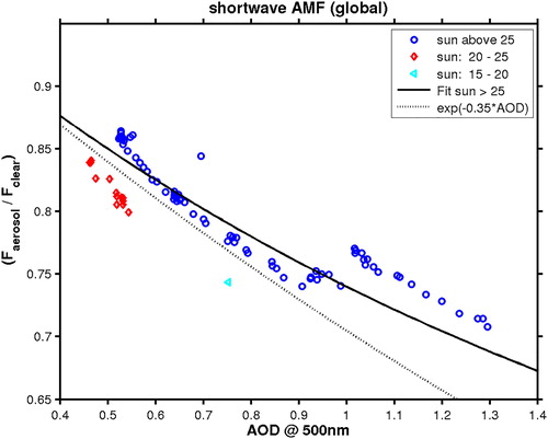
Fig. 17. Aerosol modification factor for longwave (global) radiation as a function of AOD.

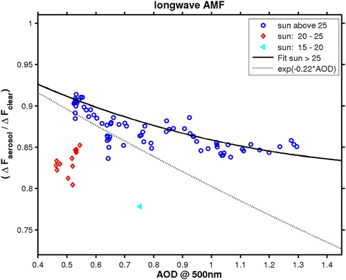
Fig. 18. Aerosol forcing as a function of AOD.

References

- Ackermann, J. 1998. The extinction-to-backscatter ratio of tropospheric aerosol: A numerical study. J. Atmos. Oceanic Technol. 15, 1043–1050. doi:10.1175/1520-0426(1998)015<1043:TETBRO>2.0.CO;2.
- Alados-Arboledas, L., Müller, D., Guerrero-Rascado, J. L., Navas-Guzman, F., Perez-Ramirez, D. and co-authors. 2011. Optical and microphysical properties of fresh biomass burning aerosol retrieved by Raman lidar, and star‐and sun‐photometry. Geophys. Res. Lett. 38, L01807. doi:10.1029/2010GL045999.
- Alexandrov, M. D., Marshak, A., Cairns, B., Lacis, A. A. and Carlson, B. E. 2004. Automated cloud screening algorithm for MFRSR data. Geophys. Res. Lett. 31, L04118. doi:10.1029/2003GL019105.
- Ansmann, A.,Wandinger, U.,Riesbell, M.,Weitcamp, C., and Michaelis, W. 1992. Independent measurements of extinction and backscatter profiles in cirrus clouds by using a combined Raman elastic-backscatter lidar. Appl Opt. 31, 7113–7131. doi:10.1364/AO.31.007113.
- Anton, M., Valenzuela, A., Mateos, D., Alados, I., Foyo-Moreno, I. and co-authors. 2014. Longwave aerosol radiative effects during an extreme desert dust event in southeastern Spain. Atmos. Res. 149, 18–23. doi:10.1016/j.atmosres.2014.05.022.
- Böckmann, C. 2001. Hybrid regularization method for the ill-posed inversion of multiwavelength lidar data in the retrieval of aerosol size distributions. Appl. Opt. 40, 1329–1342. doi:10.1364/AO.40.001329.
- Böckmann, C. and Osterloh, L. 2014. Runge-Kutta type regularization method for inversion of spheroidal particle distribution from limited optical data. Inverse Probl.. Sci. Eng. 22, 150–165. doi:10.1080/17415977.2013.830615.
- Böckmann, C., Mironova, I., Müller, D., Schneidenbach, L. and Nessler, R. 2005. Microphysical aerosol parameters from multiwavelength lidar. J. Opt. Soc. Am. A 22, 518–528. doi:10.1364/JOSAA.22.000518.
- Böckmann, C., Ritter, C. and Ortiz-Amezcua, P. 2017. Arctic biomass burning aerosol event microphysical property retrieval. In: EPJ Web Conference, Vol 176, 2018, 28th International Laser Radar Conference (ILRC28). Bucharest, Romania, 05023. doi:10.1051/epjconf/201817605023.
- Boucher, O., Randall, D., Artaxo, P., Bretherton, C., Feingold, G., Forster, P. and co-authors. 2013. Clouds and aerosols. In: Climate Change 2013: The Physical Science Basis. Contribution of Working Group to the Fifth Assessment Report of the Intergovernmental Panel on Climate Change (ed. Stocker et al.). Cambridge University Press, Cambridge, United Kingdom and New York, NY, USA, Chapter 7, pp. 571–658. doi:10.1017/CBO9781107415324.016.
- Bush, B. C. and Valero, F. P. J. 2003. Surface aerosol radiative forcing at Gosan during the ACE-Asia campaign. J. Geophys. Res. 108, 8660. doi:10.1029/2002JD003233.
- Chen, W. N., Chiang, C. W. and Nee, J. B. 2002. Lidar ratio and depolarization ratio for cirrus clouds. Appl. Opt. 41, 6470. doi:10.1364/AO.41.006470.
- Doherty, S. J., Anderson, T. L. and Charlson, R. J. 1999. Measurement of the lidar ratio for atmospheric aerosols with a 180 degree backscatter nephelometer. Appl. Opt. 38, 1823–1832. doi:10.1364/AO.38.001823.
- Eck, T. F., Holben, B. N., Reid, J. S., Sinyuk, A., Hyer, E. J. and co-authors. 2009. Optical properties of boreal region biomass burning aerosols in central Alaska and seasonal variation of aerosol optical depth at an Arctic coastal site. J. Geophys. Res. 114, D11201. doi:10.1029/2008JD010870.
- Engelhart, G. J., Hennigan, C. J., Miracolo, M. A., Robinson, A. L. and Pandis, S. N. 2012. Cloud condensation nuclei activity of fresh primary and aged biomass burning aerosol. Atmos. Chem. Phys. 12, 7285–7293. doi:10.5194/acp-12-7285-2012.
- Ferrare, R. A., Turner, D. D., Heilman Brasseur, L., Feltz, W. F., Dubovik, O. and co-authors. 2001. Raman lidar measurements of the aerosol extinction-to-backscatter ratio over the Southern Great Plains. J. Geophys. Res. 106, 20333–20347. doi:10.1029/2000JD000144.
- Haarig, M., Ansmann, A., Gasteiger, J., Kandler, K., Althausen, D. and co-authors. 2017. Dry versus wet marine particle optical properties: RH dependence of depolarization ratio, backscatter, and extinction from multiwavelength lidar measurements during SALTRACE, Atoms. Atmos. Chem. Phys. 17, 14199–14217. doi:10.5194/acp-17-14199-2017.
- Haywood, J. M., Osborne, S. R., Francis, P. N., Keil, A., Formenti, P. and co-authors. 2003. The mean physical and optical properties of regional haze dominated by biomass burning aerosol measured from the C-130 aircraft during SAFARI 2000. J. Geophys. Res. Atmos. 108, 8473. doi:10.1029/2002JD002226.
- Herber, A., L., Thomason, W., Gernandt, H., Leiterer, U., Nagel, D. and co-authors. 2002. Continuous day and night aerosol optical depth observations in the Arctic between 1991 and 1999. J. Geophys. Res. 107, AAC 6-1–AAC 6-13 doi:10.1029/2001JD000536.
- Hobbs, P. V., Reis, J. S., Kotchenruther, R. A., Ferek, R. J. and Weiss, R. 1997. Direct radiative forcing by smoke from biomass burning. Science 275, 1777–1778. doi:10.1126/science.275.5307.1777.
- Hoffmann, A. 2011. Comparative aerosol studies based on multi-wavelength Raman LIDAR at Ny-Ålesund, Spitsbergen, PhD Thesis Uni. Potsdam.
- Hoffmann, A., Osterloh, L., Stone, R., Lampert, A., Ritter, C. and co-authors. 2012. Remote sensing and in-situ measurements of tropospheric aerosol, a PAMARCMiP case study. Atmos. Environ. 52, 56–66. doi:10.1016/j.atmosenv.2011.11.027.
- Kasten, F. 1969. Visibility forecast in the phase of pre-condensation. Tellus 21, 631–635. doi:10.3402/tellusa.v21i5.10112.
- Lisok, J., Rozwadowska, A., Pedersen, J. G., Markowicz, K. M., Ritter, C. and co-authors. 2018. Radiative impact of an extreme Arctic biomass-burning event. Atmos. Chem. Phys. 18, 8829–8848. doi:10.5194/acp-18-8829-2018.
- Lv, M., Liu, D., Li, Z., Mao, J., Sun, Y. and co-authors. 2017. Hygroscopic growth of atmospheric aerosol particles based on lidar, radiosonde, and in situ measurements: Case studies from the Xinzhou field campaign. J. Quant. Spectrosc. Radiat. Tran. 188, 60–70. doi:10.1016/j.qsrt.2015.12.029.
- Markowicz, K. M., Flatau, P. J., Remiszewska, J., Witek, M., Reid, E. A. and co-authors. 2008. Observations and modeling of the surface aerosol radiative forcing during UAE. J. Atmos. Sci. 65, 2877–2891. doi:10.1175/2007JAS2555.1.
- Markowicz, K. M., Pakszys, P., Ritter, C., Zielinski, T., Udisti, R., and co-authors. 2016. Impact of North American intense fires on aerosol optical properties measured over the European Arctic in July 2015. J. Geophys. Res. 121, 14487–14512. doi:10.1002/2016JD025310.
- Maturilli, M. 2016. Basic and other measurements of radiation at station Ny-Alesund (2015-07). Alfred Wegener Institute - Research Unit Potsdam, PANGAEA. doi:10.1594/PANGAEA.863270.
- Maturilli, M. and Kayser, M. 2017. Arctic warming, moisture increase and circulation changes observed in the Ny-Ålesund homogenized radiosonde record. Theor. Appl. Climatol. 130, 1. doi:10.1007/s00704-016-1864-0.
- Maturilli, M., Herber, A. and König-Langlo, G. 2015. Surface radiation climatology for Ny-Ålesund, Svalbard (78.9°N), basic 30 observations for trend detection. Theor. Appl. Climatol. 120, 331–339. doi:10.1007/s00704-014-1173-4.
- Moroni, B., Cappelletti, D., Crocchianti, S., Becagli, S., Caiazzo, L. and co-authors. 2017. Morphochemical characteristics and mixing state of long range transported wildfire particles at Ny-Ålesund (Svalbard Islands). Atmos. Environ. 156, 135–145. doi:10.1016/j.atmosenv.2017.02.037.
- Müller, D., Ansmann, A., Mattis, I., Tesche, M., Wandinger, U. and co-authors. 2007b. Aerosol-type-dependent lidar ratios observed with Raman lidar, 2007. J. Geophys. Res. 112, D16202. doi:10.1029/2006JD008292.
- Müller, D., Böckmann, C., Kolgotin, A., Schneidenbach, L., Chemyakin, E. and co-authors. 2016. Microphysical particle properties derived from inversion algorithms developed in the framework of EARLINET. Atmos. Meas. Tech. 9, 5007–5035. doi:10.5194/amt-9-5007-2016.
- Müller, D., Mattis, I., Ansmann, A., Wandinger, U., Ritter, C. and co-authors. 2007a. Multiwavelength Raman lidar observations of particle growth during long-range transport of forest-fire smoke in the free troposphere. Geophys. Res. Lett. 34, L05803. doi:10.1029/2006GL027936.
- Ortiz-Amezcua, P., Luis Guerrero-Rascado, J., Jose Granados-Munoz, M., Antonio Benavent-Oltra, J., Böckmann, C. and co-authors. 2017. Microphysical characterization of long-range transported biomass burning particles from North America at three EARLINET stations. Atmos. Chem. Phys. 17, 5931–5946. doi:10.5194/acp-17-5931-2017.
- Penner, J. E., Dickinson, R. E. and O'Neill, C. A. 1992. Effects of aerosol from biomass burning on the global radiation budget. Science 256, 1432–1433. doi:10.1126/science.256.5062.1432.
- Pornsawad, P., Böckmann, C., Ritter, C. and Rafler, M. 2008. Ill-posed retrieval of aerosol extinction coefficient profiles from Raman lidar data by regularization. Appl. Opt. 47, 1649–1661. doi:10.1364/AO.47.001649.
- Reid, J. S., Koppmann, R., Eck, F. and Eleuterio, D. P. 2005. A review of biomass burning emissions part II: intensive physical properties of biomass burning particles. Atmos. Chem. Phys. 5, 799–825. doi:10.5194/acp-5-799-2005.
- Ritter, C., Neuber, R., Schulz, A., Markowicz, K. M., Stachlewska, I. S. and co-authors. 2016. Raman-lidar derived aerosol properties over Ny-Ålesund, Spitsbergen during the Arctic Haze season 2014. Atmos. Environ. 141, 1–19. doi:10.1016/j.atmosenv.2016.05.053.
- Samaras, S., Nicolae, D., Böckmann, C., Vasilescu, J., Binietoglou, I. and co-authors. 2015. Using Raman-lidar-based regularized microphysical retrievals and Aerosol Mass Spectrometer measurements for the characterization of biomass burning aerosols. Comput. Phys. 299, 156–174. doi:10.1016/j.jcp.2015.06.045.
- Schkolnik, G., Chand, D., Hoffer, A., Andreae, M. O., Erlick, C. and co-authors. 2007. Constraining the density and complex refractive index of elemental and organic carbon in biomass burning aerosol using optical and chemical measurements. Atmos. Environ. 41, 1107–1118. doi:10.1016/j.atmosenv.2006.09.035.
- Schulz, M., Textor, C., Kinne, S., Balkanski, Y., Bauer, S. and co-authors. 2006. Radiative forcing by aerosols as derived from the AeroCom present-day and pre-industrial simulations. Atmos. Chem. Phys. 6, 5225–5246. doi:10.5194/acp-6-5225-2006.
- Stevens, B. 2015. Rethinking the lower bound on aerosol radiative forcing. J. Clim. 28, 4794–4819. doi:10.1175/JCLI-D-14-00656.1.
- Stier, P., Schutgens, N. A. J., Bellouin, N., Bian, H., Boucher, O. and co-authors. 2013. Host model uncertainties in aerosol radiative forcing estimates: results from the AeroCom prescribed intercomparison study. Atmos. Chem. Phys. 13, 3245–3270. doi:10.5194/acp-13-3245-2013.
- Stock, M. 2010. Characterization of tropospheric aerosol variability in the European Arctic, PhD Thesis Uni. Potsdam 2010. http://opus.kobv.de/ubp/volltexte/2010/4920/.
- Stock, M., Ritter, C., Aaltonen, V., Aas, W., Handorff, D. and co-authors. 2014. Where does the optically detectable aerosol in the European Arctic come from? Tellus B 66, 21450. doi:10.3402/tellusb.v66.21450.
- Stocker, T.F., Qin, D., Plattner, G.-K., Tignor, M., Allen, S.K., et al. (eds.). 2013. IPCC, 2013: Climate Change 2013: The Physical Science Basis. Contribution of Working Group I to the Fifth Assessment Report of the Intergovernmental Panel on Climate Change. Cambridge University Press, Cambridge, United Kingdom and New York, NY, 1535 pp. doi:10.1017/CBO9781107415324.
- Toledano, C., Cachorro, V., Gausa, M., Stebel, K., Aaltonen, V. and co-authors. 2012. Overview of Sun photometer measurements of aerosol properties in Scandinavia and Svalbard. Atmos. Environ. 52, 18–28. doi:10.1016/j.atmosenv.2011.10.022.
- Tomasi, C., Kokhanovsky, A. A., Lupi, A., Ritter, C., Smirnov, A. and co-authors. 2015. Aerosol remote sensing in polar regions. Earth-Sci. Rev. 140, 108–157. doi:10.1016/j.earscirev.2014.11.001.
- Treffeisen, R., Tunved, P., Ström, J., Herber, A., Bareiss, J. and co-authors. 2007. Arctic smoke – aerosol characteristics during a record smoke event in the European Arctic and its radiative impact. Atmos. Chem. Phys. 7, 3035–3053. doi:10.5194/acp-7-3035-2007.
- Tunved, P., Ström, J. and Krejci, R. 2013. Arctic aerosol life cycle: linking aerosol size distributions observed between 2000 and 2010 with air mass transport and precipitation at Zeppelin station, Ny-Ålesund, Svalbard. Atmos. Chem. Phys. 13, 3643–3660. doi:10.5194/acp-13-3643-2013.
- van de Hulst, H. C. 1981 “Light scattering by small particles” Dover Books. (corrected reprint of the John Wiley & Sons, Inc., New York, 1957 edition). ISBN: 0-486-64228-3,
- Veselovskii, I., Kolgotin, A., Griaznov, V., Müller, D., Wandinger, U. and co-authors. 2002. Inversion with regularization for the retrieval of tropospheric aerosol parameters from multiwavelength lidar sounding. Appl. Opt. 41, 3685–3699. doi:10.1364/AO.41.003685.
- Wandinger, U., Müller, D., Böckmann, C., Althausen, D., Matthias, V. and co-authors. 2002. Special Section: Lindenberg aerosol chracterization experiments (LACE): LAC 7 optical and microphysical characterization of biomass-burning and industrial-pollution aerosols from multiwavelength lidar. J. Geophys. Res.-Part D-Atmos. 107, LAC 7-1–LAC 7-20. doi:10.1029/2000JD000202.
- Zieger, P., Fierz-Schmidhauser, R., Gysel, M., Ström, J., Henne, S. and co-authors. 2010. Effects of relative humidity on aerosol light scattering in the Arctic. Atmos. Chem. Phys. 10, 3875–3890. doi:10.5194/acp-10-3875-2010.
- Zieger, P., Weingartner, E., Henzing, J., Moerman, M., Leeuw, G. D. and co-authors. 2011. Comparison of ambient aerosol extinction coefficients obtained from in-situ, MAX-DOAS and LIDAR measurements at Cabauw. Atmos. Chem. Phys. 11, 2603–2624. doi:10.5194/acp-11-2603-2011.