Changes in vaginal community state types reflect major shifts in the microbiome

ABSTRACT

Background: Recent studies of various human microbiome habitats have revealed thousands of bacterial species and the existence of large variation in communities of microorganisms in the same habitats across individual human subjects. Previous efforts to summarize this diversity, notably in the human gut and vagina, have categorized microbiome profiles by clustering them into community state types (CSTs). The functional relevance of specific CSTs has not been established.

Objective: We investigate whether CSTs can be used to assess dynamics in the microbiome.

Design: We conduct a re-analysis of five sequencing-based microbiome surveys derived from vaginal samples with repeated measures.

Results: We observe that detection of a CST transition is largely insensitive to choices in methods for normalization or clustering. We find that healthy subjects persist in a CST for two to three weeks or more on average, while those with evidence of dysbiosis tend to change more often. Changes in CST can be gradual or occur over less than one day. Upcoming CST changes and switches to high-risk CSTs can be predicted with high accuracy in certain scenarios. Finally, we observe that presence of Gardnerella vaginalis is a strong predictor of an upcoming CST change.

Conclusion: Overall, our results show that the CST concept is useful for studying microbiome dynamics.

Introduction

The human microbiome consists of many microorganism communities that reside in various body habitats. While the presence of human microbiomes has been documented for several decades, there has been a recent surge of research linking the microbiome with human health and disease. This growth in microbiome-related knowledge has been facilitated primarily by next-generation sequencing; specifically, sequencing of 16S ribosomal RNA enables quantification of relative abundance of the different species residing in these environments. As microbiome profiling has revealed large variation among individuals and over time, efforts have been made to categorize or cluster microbiome profiles into a small number of community state types (CSTs).

Previous studies have used CSTs to summarize the microbial communities observed in the human vagina and the human gut. Vagitypes [1] are widely used as prototypes in the interpretation of vaginal microbiome data,[1–6] while enterotypes are somewhat more controversial [7] as prototypes for the gut microbiome.[8,9] Despite their common usage, it is not well established whether CSTs indeed represent fundamental biological states and whether they can provide valuable clinical information.

In this paper we investigate the stability of CSTs across different datasets and their predictive ability especially with respect to microbial shifts. We concentrate on CSTs since they offer a reduction in data complexity that has the potential to facilitate subsequent analysis and discovery, and they also simplify the interpretation of high-dimensional data for possible clinical decision support. Establishing their utility in diagnostics and discovery has potential benefits for microbiome research.

A variety of normalization methods have been suggested for microbiome sequence counts data, and there are many options for clustering procedures for defining CSTs. Choices in normalization and clustering methods can lead to artifacts when evaluating specific datasets with respect to CSTs. Though CSTs have been used in the literature, they have not been evaluated rigorously, either statistically or clinically.

CSTs have the potential to be useful clinically, especially for assessment of bacterial vaginosis (BV), the most common cause of vaginitis. A single species often dominates the vaginal microbiome, which has implications for vaginal health. For example, Lactobacillus species are often a majority among bacteria; they consume glycogen from the epithelium and produce lactic acid, thereby lowering the pH of the vagina and preventing colonization by pathogens. Among lactobacilli, Lactobacillus iners is considered among the least protective in part because it is associated with a higher pH and can co-occur with BV-associated bacteria.[10,11] Species such as Gardnerella vaginalis,[12–15] Sneathia amnii,[16,17] BVAB1,[18] and other non-lactobacilli are associated with dysbiosis. BV is generally characterized by low levels of Lactobacillus spp. and/or an increase in Gram-negative anaerobes. BV is highly recurrent, with recurrence occurring in up to 60% of subjects within one year. Moreover, up to 84% of women may have a shift in vaginal microbiota associated with BV without clinical symptoms.[19] Given the polymicrobial nature of BV infection, we investigate if changes in vaginal microbial composition over time may be used to predict BV infection or recurrence by indicating upcoming shifts to high-risk states. Changes in the microbial community composition may be precursors to changes in health, and may provide more etiologic information regarding prognosis.

In this work we provide an in-depth analysis of CSTs of the vaginal microbiome to assess their predictive value. Rather than assessing which CST method is best at reflecting clinical data, we first demonstrate that detecting major shifts in the microbiome as indicated by CST transitions is largely independent of the CST definition method. We then evaluate whether there is a similarity across datasets in patterns that are suggestive of mechanisms for shifts in microbial flora, and whether CSTs can be used as a tool to discover mechanisms involved in such shifts. Specifically, we analyze the time scales of CST transitions, the expected persistence of a particular CST, the frequency of transitions between CSTs, the relationship of CST with changes in Nugent score and pH, the ability to predict CST transitions, and the bacteria that may be harbingers of CST transitions. Our findings demonstrate that vaginal CSTs are predictive of changes in the future bacterial environment.

Materials and methods

Data sources

We used five datasets that have two or more longitudinal vaginal samples per subject for this analysis. Four of the datasets are derived from amplicon-based surveys and one is based on whole metagenome shotgun sequencing (WMGSS). The studies employed different protocols and include varying amounts of clinical data so that a pooled analysis is not possible.

The amplicon-based datasets were generated by 454 pyrosequencing while the WMGSS data was generated by Illumina sequencing. The datasets will be referred to as: ravel,[2] gajer,[3] chaban,[20] hmp,[21] and vahmp,[22] where the names correspond to prefixes in the data structures in the R code. The R code and output are in Supplemental Files 1–6, and the data except for the vahmp data are in Supplemental File 7. Sources and characteristics of the datasets are contained in Table 1. All studies included non-pregnant healthy women of reproductive age; two of the datasets also included women with diagnoses of BV. Each dataset includes species-level assignments of reads based on alignment to a reference database.

Table 1. Datasets used in analysis.

	ravel [2]	gajer [3]	chaban [20]	hmp [21]	vahmp [22]
Sampling frequency	Daily	Twice-weekly	Weekly	1–11 months	1–32 months
Gene	16S	16S	cpn60	N/A (WMGSS)	16S
Region	V1–V3	V1–V2		N/A	V1–V3
No. of subjects	25	32	27	63	141
Samples per subject	59–70	27–33	2–4	2–3	2
Primers	27f, 533r	27f, 338r	H279/H280, H1612/H1613	N/A (WMGSS)	Custom (see [26])
Median library size	5093	2403	4638	N/A	27,130
No. of samples	1657	937	76	152	282
No. of taxa/OTUs	151	330	73	321	247

The ravel dataset comprises data collected daily over two menstrual cycles obtained from 25 women of reproductive age via self-sampling, yielding a total of 1657 samples. Of the 25 women, 15 were diagnosed with symptomatic BV according to the Amsel criteria [23] and self-reported symptoms, six were diagnosed with asymptomatic BV, and four received no diagnosis throughout the course of the study. We exclude from our analysis data from time points for which sequence information is not available, including 10 samples from eight subjects at times corresponding to diagnoses of symptomatic BV and 21 samples from 13 subjects at times corresponding to diagnoses of asymptomatic BV. We considered samples to be consecutive for evaluating CST changes if they were collected one day apart.

The gajer dataset comprises data from 32 women who self-sampled twice weekly for 16 weeks as part of a douching cessation study.[24] Women were of reproductive age, healthy and not pregnant throughout the study. Each woman reported that she had used douching products in the two months prior to the study, and that she had a regular menstrual cycle. Use of douching products was continued through the first four weeks, and stopped for the remaining 12 weeks. We considered samples to be consecutive for evaluating CST changes if there were six days or less between collections.

The chaban dataset comprises data from clinician-collected samples from 27 women. Microbial sequence data are available for two to four samples per subject collected weekly. Exclusion criteria included pregnancy, autoimmune conditions, use of hormonal contraceptives, use of antibiotic or antifungal medications, and irregular menstrual cycles.

The hmp dataset comprises data from two or three clinician-collected samples from 63 women separated by 1–11 months. Volunteers were between 18 and 40 years of age, and had passed a screening that included exclusion criteria for pregnancy, high or low body mass, oral health, drug use, and history of cancer. The sequence data were processed using MetaPhlAn2 [25] to generate relative abundances of taxa at different levels of resolution. For this study, we used only species-level proportions.

The vahmp dataset comprises data from two clinician-collected samples from 141 women separated by 1–31 months. Pregnant subjects were excluded. Of 282 samples, 90 (31.9%) were associated with a diagnosis of BV by the Amsel criteria at the time of collection. The remaining samples were not associated with any diagnosis.

Data analysis

Unless otherwise noted, analysis was performed and visualizations created using the R language and environment for statistical computing,[27] including packages Biobase,[28] compositions,[29] DESeq2,[30] edgeR,[31] entropy,[32] expm,[33] ggplot2,[34] gridExtra,[35] knitr,[36] markovchain,[37] mcc,[38] msm,[39] phyloseq,[40] pROC,[41] randomForest,[42] reshape2,[43] rgl,[44] rglwidget,[45] and sigclust2.[46]

Results

Identifying community state types

CSTs are usually defined using hierarchical clustering based on a dissimilarity measure.[3,10,20] For each dataset, we used pairwise Bray–Curtis (BC) dissimilarities as the input to clustering; the profiles consisted of taxa proportions for each sample. As in previous studies of the vaginal microbiome where samples were clustered into five CSTs,[3,10,20] we used Ward’s method for hierarchical clustering which creates clusters that result in the smallest increase in total within-cluster variance, measured as the sum-of-squared Euclidean distances between points.[47]

Scree plots for the within-cluster distances (Supplemental File 2) indicate that the distances drop noticeably after 4–5 clusters. However, for none of the datasets does the scree plot have a sharp bend in the curve denoting a clear indication of the number of naturally-occurring clusters.

Characteristic taxa of CSTs

Figure 1 summarizes the CST assignments for each of the datasets; Table 2 summarizes CST assignments and compares them to the CSTs identified in [3,10]. Roman numerals are used to denote the CSTs defined in [3,10] and Arabic numerals are used to denote the CSTs based on our clustering.

Table 2. Summary of community state types for data with species-level taxonomic assignments.

Characteristic taxa	CST # in [3,10]	Our CST #	% of samples
			ravel [2]	gajer [3]	chaban [20]	hmp [21]	vahmp [22]
L. crispatus	I	1	8.6	18.1	38.2	48.7	17.0
L. gasseri	II	2		5.9		5.9
L. iners	III	3	26.9	36.9	26.3	29.6	27.0
Various	IV-A	4-A		6.5	10.5		11.0
A. vaginae	IV-B	4-B		32.4
L. jensenii	V	5	7.1		15.7	6.6
G. vaginalis	NA	6	29.6			9.2	32.6
BVAB1	NA	7					12.4
B. breve	NA	8			9.2
L. iners and
G. vaginalis	NA	9	27.9

Figure 1. Community state types. Stacked bar plot of bacteria present in microbiome samples grouped by community state type (CST) for the (a) ravel,[10] (b) gajer,[3] (c) chaban,[20] (d) hmp,[21] and (e) vahmp [22] datasets. Each sample is represented by a bar along the x-axis and the proportion of reads assigned to each taxon is indicated by the colors in the bar. Key for major taxa: L. crispatus (yellow), L. iners (light blue), G. vaginalis (red), A. vaginae (brown), Lachnospiraciae BVAB1 (orange), Bifidobacterium (light green). Samples are ordered by CST, and the assigned CST number is given on the x-axis of each plot. Table 2 contains a summary of the CSTs.

Most CSTs are characterized by a single predominant bacterium. CST 1 contains samples that are mostly comprised of L. crispatus and few other bacteria. This CST, common to all datasets, would traditionally be considered low risk because of the protective role of L. crispatus and low diversity. Samples assigned to CST 3 contain mostly L. iners.

The ravel and vahmp datasets were the only datasets with samples from subjects receiving a diagnosis of BV, and have unique CSTs. For these datasets, the CST with the most samples is CST 6, characterized by G. vaginalis. The ravel dataset has a CST associated with the presence of G. vaginalis and L. iners (CST 9), and the vahmp dataset has a CST associated with BVAB1 (CST 7).

Other bacteria that are common in certain CSTs but not others across the datasets include L. jensenii, L. gasseri, Atopobium, Bifidobacterium, Fusobacterium, and S. agalactiae (Group B Streptococcus – GBS).

Many samples are assigned to CSTs that are not characterized by the lactobacilli that are traditionally associated with vaginal health (L. crispatus and L. gasseri). At the same time, relatively few samples are associated with a diagnosis of BV. Microbiome profiles such as these could contain leading indicators of dysbiosis.

Agreement with previously-defined CSTs

The gajer dataset [3] included CST assignments. We compared our CST assignments to those in the original study.

Ravel et al. [10] first identified five CSTs that are distinguishable by whether they are dominated by lactobacilli and the Lactobacillus species present. The CSTs were dominated by L. crispatus in I, L. gasseri in II, L. iners in III, no Lactobacillus species in IV, and L. jensenii in V. In a longitudinal study, Gajer et al. [3] assigned samples from subjects to CSTs characterized by L. crispatus dominance for I, L. gasseri dominance for II, L. iners dominance for III, presence of L. crispatus and/or L. iners but no dominance for IV-A, and very little lactobacilli for IV-B.

Our CST assignments for the gajer data have 92.6% agreement with the CSTs assigned in the original publication.[3] The discrepancies are in our assignment of samples to CSTs originally assigned to CST III, CST IV-A and CST IV-B (Supplemental File 2).

Agreement across CST definition methods

We investigated how different choices for normalization and clustering for defining CSTs would affect the detection of a change in CST. We considered five methods: hierarchical clustering using BC dissimilarities, hierarchical clustering using Jensen–Shannon divergences of counts normalized using DESeq2,[30] hierarchical clustering using Jensen–Shannon divergences of proportions, a method based on the predominant taxon in each sample, and hierarchical clustering using the biological coefficient of variation (BCV) [48] (Supplemental Files 1 and 3). When data were normalized using DESeq2, a pseudo-count of 1 was added to the number of bacterial reads for each taxon. The method based on the predominant taxon assigns a CST to a sample based on the taxon for which the most reads were observed, provided that it comprises at least 30% of the sample; otherwise, no CST is assigned.[1] BCV measures dissimilarity while accounting for overdispersion.[49]

Table 3 summarizes the agreement among different CST assignment methods in identifying CST changes for the gajer data. The entry in each column indicates the proportion of transitions agreeing or disagreeing with the CST transitions reported by Gajer et al. [3]. The agreement is 78–92% across the different methods for defining CSTs (obtained by adding the diagonal elements for each CST method in Table 3). The method using BC dissimilarities agreed the most. Identifying the ‘best’ method is not possible because there is no ground truth for CST assignment. The analyses discussed in the remainder of the paper are based on BC dissimilarities.

Table 3. Agreement of CST transitions for different CST assignment methods.

CST definition method		Original publication [3]
		Transition	No transition
Clustering Based on	Transition	13.9%	2.6%
Bray–Curtis Dissimilarity	No transition	4.9	78.5
Hierarchical Clustering	Transition	13.3	2.9
Based on Jensen–Shannon Divergences	No transition	5.4	78.3
Hierarchical Clustering	Transition	13.7	4.2
of DESeq2-normalized counts	No transition	5.1	77.1
Clustering Based on	Transition	15.6	7.3
Predominant Taxon	No transition	3.2	74.0
Hierarchical Clustering	Transition	7.9	11.1
of BCV Distances	No transition	10.9	70.1

The time scale and persistence of community state types

Longitudinal data can provide insight into the frequency of CST transitions, the length of time between transitions, and the expected amount of time that a subject remains in a particular CST. Differences in persistence based on CST have been observed but not quantified.[3,5,50,51]

CST transitions can occur on short time scales

For the gajer dataset, Figure 2(a) contains a plot of the BC dissimilarities between microbiome profiles and the microbiome profile after the next CST change as a function of the number of days until the next CST change. Dissimilarities are normalized by subject by subtracting the mean and dividing by the standard deviation. The mean and standard deviation for five-day bins are plotted. If CST transitions occurred gradually, we would expect the average distance and the standard deviation to decrease as the day of a change approaches, indicating that samples make consistent movements towards the profile assigned to the new CST. In the figure we see that while there may be a slight trend to decreasing distance to the new CST over the 10–20 days preceding a transition, the variance in distance actually increases as a CST change approaches. Similar results are seen for the ravel dataset (Supplemental File 4). These results suggest that CST changes can reflect either abrupt shifts in microbiome profiles over less than a week or that they can reflect gradual changes, but not one or the other exclusively.

Figure 2. Persistence of CST states. (a) Plot of mean and standard deviation of five-day bins of z-scores of distances of microbiome profiles from profiles at the next CST change for the gajer [3] data, as a function of the days until the next CST change. (b) Markov chain diagram indicating the probability of transitioning between states in one week for the gajer dataset.

Frequency of CST transitions depends on the current CST

We fit continuous-time Markov chain models to derive per-day CST transition rates and the expected time spent in each state before leaving for another state (persistence) for the daily (ravel), twice-weekly (gajer), and weekly sampled (chaban) data.

Throughout this section we report point estimates and 95% confidence intervals. Note that the confidence intervals for transition probabilities are calculated based on the log of the intensities, and therefore may not be symmetric about the point estimate.

Persistence refers to the tendency of a subject’s samples to remain in a CST. For the gajer data, the probability of remaining in a given state over the course of a week is 0.38 (0.22,0.50) for CST 4-A and at least 0.72 (0.61,0.79) for other CSTs (Figure 2(b)). High probabilities for remaining in the current state are seen for the chaban dataset, ranging from 0.60 (0.11,0.89) for CST 4-A to an observed absorbing state for CST 8. For the ravel dataset, which included several women diagnosed with BV, the probabilities for remaining in a given state over the course of a week were lower, and ranged between 0.38 (0.31,0.44) for CST 9 to 0.48 for CSTs 3, 5, and 6 ((0.37,0.55), (0.25,0.63), (0.37,0.55)).

The expected number of days remaining in the current CST depends on the CST. For most CSTs, subjects spend one to three weeks in a given state. CST 6 for the ravel dataset, characterized by a mix of L. iners and G. vaginalis, had an expected persistence of 4.1 ± 0.80 days. Other CSTs in that dataset have expected sojourn times of approximately one week. For the healthy cohorts in the gajer and chaban datasets, the expected sojourn times are more than two weeks with one exception in each dataset. CST 4-A in the gajer and chaban datasets, characterized by high diversity, have expected persistences of 6.8 ± 2.7 days and 13.9 ± 19.4 days, respectively.

Across the three datasets, the probability of transition to a CST 3 characterized by L. iners was among the highest transition probabilities. For the ravel dataset, the highest probabilities of transition were among CSTs 3, 6, and 9, which are characterized by L. iners and G. vaginalis. The weekly transition probabilities are between 0.15 (0.11,0.21) and 0.33 (0.26,0.38) for these CSTs. For the gajer dataset, the highest transition probabilities were for transitions to CST 3 (up to 0.21 (0.12,0.36)), characterized by L. iners, and from CST 3 and CST 4-A to high-risk CST 4-B (0.12 (0.080,0.17) and 0.16 (0.083,0.30)), characterized by A. vaginae. For the chaban dataset, the highest transition probabilities were for transitions to CST 3 (up to 0.35 (0.09,0.76)) and from CST 3 to low-risk CST 1 (0.21 (0.067,0.46)), characterized by L. crispatus. Across the three datasets, the transition probabilities to CST 3 were lowest for low-risk CSTs 2, 5, and 1 which are characterized by L. gasseri, L. jensenii, and L. crispatus, respectively (Supplemental File 4).

The ravel dataset includes an indication of days on which BV medication was taken. Among samples corresponding to a woman’s first day of treatment, three women were in CST 3, three were in CST 6, and seven were in CST 9 before medication began. Eleven of the samples collected after medication stopped were in CST 3 (characterized by L. iners), one transitioned to CST 9 (characterized by L. iners and G. vaginalis), and one transitioned to CST 1 (characterized by L. crispatus). We fit a continuous-time Markov chain for the ravel data with BV medication as a covariate for transitions from CST 6 to 3 and from CST 9 to 3. For samples corresponding to medication days, the probabilities of transitioning to (lower-risk) CST 3 were higher (0.19 (0.055,0.88) versus 0.014 (0.0082,0.033) and 0.65 (0.40,0.86) versus 0.073 (0.054,0.099) for one-day transitions.

Dynamic modeling of community state types, Nugent scores, and pH

Dynamic models can characterize the actual flow of influence between various variables and can be used to forecast outcomes at any given time in the future. A natural tool for learning dynamic models, and handling both uncertainty and complexity, is provided by dynamic Bayesian networks (DBNs).[52] This framework enables modeling of high-dimensional processes with complex dependencies that are expressed as an interpretable network topology. DBNs naturally deal with missing data, using exact inference for small topologies, and a variety of approximate methods for large topologies. In our analysis, we used the structured proportional jump process (SCUP) [53] modeling framework which combines ideas from the fields of proportional hazard models [54] and continuous-time DBNs and allows for efficient modeling of non-homogeneous multi-component processes.

Briefly, the SCUP modeling framework defines, for an outcome i, the probability of transition from state $y_i$ at time t to state ${\bar{y}}_i$ at time $t+{\mathrm{\Delta }}_t$, where ${\mathrm{\Delta }}_t$ tends to 0, as:

(1) $Pr\left({\bar{y}}_i^{t+{\mathrm{\Delta }}_t}|y_i^t,{\mathbf{y}}_{pa(i)}^t,\mathbf{x}\right)\approx r_{y_i\to {\bar{y}}_i}^t\cdot exp\left({\mathbf{w}}_{y_i\to {\bar{y}}_i}^i\cdot \left\{\mathbf{x},{\mathbf{y}}_{pa(i)}^t\right\}\right)\cdot {\mathrm{\Delta }}_t,$(1)

where the first factor on the right-hand side is the non-negative, time-dependent baseline rate; and the second factor considers the structural context of outcome i and expresses the effect that the joint state of its parents (${\mathbf{y}}_{pa(i)}^t$) and the features (x) has on the transition rate using the weight vector ${\mathbf{w}}_{y_i\to {\bar{y}}_i}^i$. An expectation maximization (EM) procedure is employed to estimate the model parameters from point observations and partially observed data; for more details, see [53]. We estimated each parameter’s 95% confidence interval as ±1.96 times (because $P(-1.96<z<1.96)=0.95$ for $z\sim N(0,1)$) the standard deviation of the estimated parameter, computed using 250 bootstrap iterations. P-values were computed via Wald tests and FDR-adjusted to account for multiple hypothesis testing.

We used SCUP (Matlab implementation) for modeling the dynamics of CST risk level, pH and Nugent score and their dependence on age, ethnicity, BV medication, and menses. High-risk CSTs are those associated with high Nugent scores and diagnosis of BV. The high-risk CSTs are CSTs 6 and 9 in the ravel data and CST 4-B in the gajer data. The remaining CSTs were labeled low risk. pH values were discretized to binary states, using a cutoff of 4.5, up to which vaginal pH is considered normal. Nugent scores, currently the diagnostic gold standard for BV,[55,56] are calculated using Gram staining of a clinical sample. Lower Nugent scores (<4) are the result of high numbers of Lactobacillus spp. and high Nugent scores (>6) occur when there are little or no Lactobacillus spp. present. Diagnosis of BV in samples with intermediate (4–6) levels of Lactobacillus spp. requires the presence of clue cells.[55] To improve numerical stability, we normalized continuous features to have zero mean and standard deviation of one. We further expanded categorical features into a collection of indicators.

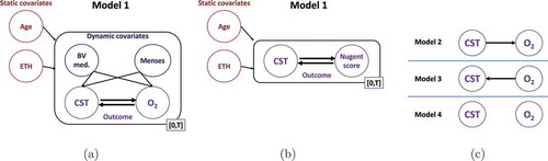
For the ravel data, we constructed models using two static features, age and ethnicity, two dynamic features whose values can change over time, BV medication and menses, and two sets of two outcomes that we wished to forecast, CST risk level and pH or Nugent score (Figure 3(a)). The gajer data did not include pH measurements, or information on BV medication and menses. Consequently, the constructed models considered only two features, age and race/ethnicity, and one set of two outcomes, CST and Nugent score (Figure 3(b)).

Figure 3. Dynamic modeling of the vaginal microbiome. Dynamic models are constructed using the (a) ravel and (b) gajer data. Each model consisted of static features age and race/ethnicity. For the ravel data, dynamic features BV medication and menses were included. (a) For the ravel data two sets of two outcomes were modeled, CST and O₂, where O₂ denotes Nugent score or pH. (b) For the gajer data, CST and Nugent score were the outcomes. (c) Unlike the other models, which assume bidirectional influence between the outcome variables, models 2–4 (right) consider unidirectional or no direct influence between the outcomes (model 4). These models were fit for each combination of static, dynamic, and outcome variables.

Modeling results for community state type, Nugent score, and pH

Using the models above, SCUP was employed to understand the influence of features on outcome transitions as well as to determine outcome-outcome dependencies; the inferred effects and effect differences for each pair of outcome states are shown in Figure 4. As expected, in both ravel models, BV medication significantly increased the rate of transition from high- to low-risk CST (p-values of 0.01 and $1.3\times {10}^{-4}$, for the pH and Nugent score models, respectively), favoring the high- to low-risk transition over the opposite one (p-values of 0.005 and ${10}^{-4}$). Menses (but not BV medication) significantly affected pH level transitions, decreasing high to low pH rate (p-value = 0.02) and preferring low to high over high to low pH transition (p-value = 0.02). In addition, race/ethnicity had a significant effect on the transition rate from low to medium Nugent score (p-value = 0.035), but the overall effect on the low $\leftrightarrow$ medium transition was not significantly different from 0, indicating that race/ethnicity, on its own, does not drive Nugent score to either level. The estimated effect of the remaining features, though in some cases large, had a large sampling variance and was not statistically significant.

Figure 4. Inferred dynamic effect. Shown are, for each model, the effects that the features and outcome have on the rate of change of the other outcome’s state (e.g. a negative H- $\to$ L-risk effect decreases the rate of change from high- to low-risk CST) as well as the associated difference in effects between each pair of outcome states (e.g. a positive L- $\leftrightarrow$ H-risk indicates an overall effect preferring H- over L-risk CST). Darker (lighter) colors indicate effects greater (less) than 0; 95% confidence intervals are given in parentheses; and * denotes effect or effect difference significantly different than 0 at a 5% significance level. L, M, H stand for low, medium and high.

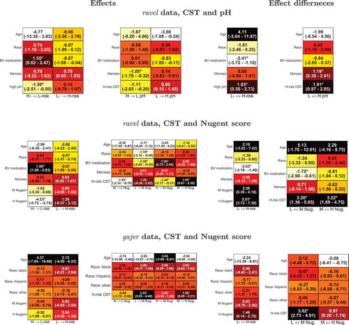
In all models, an outcome had a significant effect on the transition rates of the other one, typically stronger than that of the features. Specifically, high pH significantly increased the low- to high-risk CST transition rate compared to the high- to low-risk transition (p-value = 0.02; Figure 4, top row) and high-risk CST had an even stronger effect on low $\leftrightarrow$ high pH transition (p-value = 0.002). This is perhaps expected as high-risk CSTs contain less lactic acid-secreting bacteria. For the ravel data, high-risk CST increased the transition rates to a higher Nugent score (p-values of 0.005 and $3.7\times {10}^{-4}$ for low $\leftrightarrow$ medium and medium $\leftrightarrow$ high Nugent score transitions, respectively); and medium and high Nugent scores drove CST to high-risk level stronger than the other way around (p-values of 0.062 and $7.8\times {10}^{-8}$, respectively). Similar trends for the interdependencies between CST risk level and Nugent score were observed for the gajer data though, typically, these were associated with less significant p-values.

Assessing the most likely models

To further characterize the relationships between outcomes, we constructed four dynamic models that cover all possible relationships between each pair of outcomes (Figure 3) and calculated the out-of-sample log likelihoods of each subject using a leave-one-out approach (hence penalizing models for a greater number of parameters is unnecessary). To test the hypothesis that the observed difference in sums of out of sample log likelihoods between models is greater than 0, we repeatedly selected a random subset of subjects, switched between each subject’s log likelihoods in the two models and computed the fraction of iterations in which the observed difference is lower; we then corrected for multiple hypothesis testing, using Benjamini-Hochberg’s FDR method.

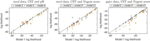
For all dynamic models, summation of the log likelihoods showed that the bidirectional dependency model, model 1, was most likely, followed by the unidirectional model 2, then model 3, and finally model 4, with no direct influence between outcomes (Figure 5). Notably, for both ravel and gajer Nugent score models, model 1 obtained significantly greater log likelihoods than the corresponding model 3 and 4 (p-values of 0.004,$1.2\times {10}^{-4}$; and $1.7\times {10}^{-4}$, $9\times {10}^{-6}$, respectively); but its advantage over model 2 was not statistically significant. These results, and CST trajectories of subjects (Supplemental File 3), seem to indicate a strong relationship between CST and Nugent score, where CST changes are accompanied by changes in Nugent score, but there may be changes in Nugent score for which there is no CST change.

Figure 5. Comparison of dynamic models to evaluate outcome relationship. For each dynamic model, the per subject out of sample log likelihoods obtained by the outcome bidirectional dependency model 1 plotted against the corresponding values computed by models incorporating unidirectional (model 2, blue, and 3, brown) or no relationship (model 4, yellow) between outcomes (see Figure 3 for definition of models). * denotes cases where the sum of model 1’s log likelihoods is significantly greater than that of the corresponding model.

Outcome variable trajectories

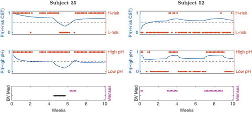
SCUP modeling enables predicting trajectories of outcome variables, from the static and dynamic features and an initial outcome configuration; two examples of such trajectories are shown in Figure 6. Clearly, the two dynamic features have a strong effect on the predicted trajectories, with BV medication more strongly affecting CST risk level and menses having a greater impact on pH levels.

Figure 6. Outcome trajectories from dynamic model 1. The CST risk (top panel) and pH level (middle) trajectories are shown for ravel’s subjects 35 (left) and 52 (right). Blue are the model predicted trajectories, red are the actual outcome values, and the dotted lines reflects equal probability of being in either outcome state. The bottom panel shows the assigned BV medication (black) and menses (cyan) values, respectively.

Predicting changes in community state type

In this section we investigate the ability to predict future CST changes and study the relationships between specific bacteria and major shifts in microbiome composition. We assess the ability to predict CST changes and CST risk level with fixed-time modeling methods. This is done using two large datasets, ravel and gajer, and across varying time horizons. Second, we evaluate the ability to predict an upcoming CST change in all five datasets. Finally, we analyze which bacteria are indicative of upcoming CST changes.

Predicting an upcoming CST change

A random forest (RF) [57] was used to evaluate the ability to predict an upcoming CST change based on current microbiome profile and clinical information. To address class imbalance, class weights were employed with each class weighted by the other’s prevalence. We compared predictions at the sampled intervals (ravel: daily; gajer: twice-weekly) to a seven-day prediction horizon. We further assessed predictions made by assigning randomly selected samples to the test set (practically, using out-of-bag predictions) to predictions made when samples from an entire trajectory of a subject were assigned to the test set. Prediction accuracy was evaluated using area under the receiver operating characteristic (ROC) curve (AUC), where a higher AUC reflects better prediction accuracy, as well as sensitivity at 80% specificity.

Random forest out-of-bag predictions for individual samples obtained AUC values of 0.72–0.86 and sensitivity of 44–73% at 80% specificity (Figure 7(a) and 7(b), left column; and Supplemental File 8). Adding clinical information had a negligible effect on the prediction accuracy (data not shown). Perhaps surprisingly, CST changes at a seven-day horizon were more accurately forecasted compared to one or three/four-day horizon, most notably for the ravel dataset. This may be partly due to the greater number of such CST changes available for training in the former case (25% vs. 14% and 19% vs. 14% for the ravel and it gajer datasets, respectively).

Figure 7. Predicting CST changes for daily and twice-weekly sampled data. (a) Receiver operating characteristic (ROC) curves showing the accuracy of random forest models on the ravel [2] data at one- and seven-day horizons (blue and red, respectively) and gajer [3] samples at 3/4- and seven-day horizons (green and cyan, respectively). The dotted black line represents the performance of a random predictor. Each curve depicts the true positive rate (or sensitivity, y-axis) versus the false positive rate (or 1 – specificity, x-axis) along the entire predictive score range; for example, the dashed vertical line and the right value in the parentheses indicate the sensitivity at 80% specificity. The area under the ROC curve (AUC, left value in parentheses) reflects the overall prediction accuracy, with higher values corresponding to better accuracy. The heatmaps show the average test AUC values for predicting (b) CST change or (c) risk level when testing on specific samples or entire subject’s trajectory and using features extracted from the microbial community data. Darker shades indicate higher AUC values; 1 d, 3/4 d, 7 d: prediction horizon of one, three/four and seven days, respectively.

When trained repeatedly on all but a single subject, RF models exhibited poorer performance (Figure 7(b), right column; and Supplemental File 8). This low prediction capability reflects the larger inter-person variation compared to intra-person variation. Here, again, clinical information did not improve prediction accuracy; and the accuracy of predicting CST changes at a seven-day horizon is comparable to the shorter horizons.

Predicting CST risk level

As noted above, we identified ravel’s CSTs 6 and 9 and gajer’s CST 4-B as high risk CSTs and trained RF models on the relative microbial abundances to predict CST risk level at one, three/four and seven-day prediction horizons, splitting the data by either samples or subjects. The inferred models, for all learning scenarios, obtained high AUCs and sensitivity values (Figure 7 and Supplemental File 8), with the lowest performing model being ravel’s seven-day horizon, obtaining an AUC of 0.85 and sensitivity of 80% at 80% specificity.

Prediction horizon and CST change prediction accuracy

Table 4 contains the AUC for prediction of an upcoming CST change for each of the five datasets using random forests and the sensitivity at 80% specificity. At a specificity of 80%, the sensitivity is approximately 50% when the prediction horizon is less than four days. The prediction performance degrades as the prediction horizon increases, but the accuracy remains above 50% for many choices of specificity across the datasets. The better-than-random accuracy for prediction horizons >30 days for both subjects changing CST and those remaining in their current CST could be an indication that subjects have a CST to which they tend to return or remain despite various environmental perturbations.

Table 4. Area under the ROC curve (AUC) and sensitivity at 80% specificity for predicting CST changes.

Dataset	Prediction horizon	AUC	Sensitivity at 80% specificity
ravel [2]	1 day	0.72	51.9%
gajer [3]	3–4 days	0.75	55.2
chaban [20]	7 days	0.49	26.3
hmp [21]	1–11 months	0.50	25.0
vahmp [22]	1–31 months	0.59	25.8

Bacteria indicative of upcoming CST changes

Two approaches were used to detect taxa/OTUs that were present in different levels between samples corresponding to CST changes and those corresponding to remaining in the same CST:

1. A test of differences in abundance based on the Benjamini–Hochberg correction [58] with the following modifications. Prior to the tests, the taxa/OTUs are given an ordering based on hierarchical clustering of the proportions using the Manhattan metric and Ward’s criteria. Taxa/OTUs found in at least five samples were included. To maximize power to detect differences in abundances by exploiting correlations in outcomes of related taxa, we employed a two-stage hidden Markov model (HMM) as proposed by Sun and Cai [59] to obtain z-statistics for differences in abundance. For finite sample sizes, z-statistics can demonstrate skew, even under the null,[60] and so we first computed highly accurate p-values for the relationship between abundance and CST transitions by performing 1 million permutations for each feature. One tailed p-values were then converted to z-statistics using the inverse quantile normal transformation, and then used for the HMM group-level FDR procedure as implemented in R.[61]

2. The method implemented in Linear Discriminant Analysis Effect Size (LEfSe).[62] The software applies a Kruskal–Wallis test, a non-parametric test, and then linear discriminant analysis to evaluate effect size.

In each dataset except for the gajer dataset, the presence of G. vaginalis is strongly associated with an upcoming CST change. For the ravel and vahmp datasets, this observation may reflect treatment for BV in these cohorts. Figure 8 depicts results for the ravel dataset from LEfSe.

Figure 8. Bar plot of effect sizes for bacteria with significant differences between subjects with a CST change in the next sample (TRUE) versus those that will remain in the current CST (FALSE) for the ravel [10] dataset.

A clear pattern for lactobacilli and CST changes does not emerge across the datasets. For several Lactobacillus species, they were associated with CST transitions in one dataset while being associated with remaining in the same CST for another. L. iners is associated with an upcoming CST change only in the ravel dataset. L. crisipatus is associated with remaining in the current CST in the ravel dataset, but is strongly associated with an upcoming change in the gajer dataset. L. gasseri is associated with an upcoming CST change for the ravel but is a predictor for remaining in the current CST for the gajer, hmp, and vahmp datasets. The presence of L. jensenii is associated with CST changes in the ravel dataset, but is associated with remaining in the same state in the hmp and vahmp datasets.

There is also disagreement across datasets for the roles of the less-prevalent community members. Atopobium spp. are associated with remaining in a CST for the ravel and gajer datasets, but is associated with CST changes in the hmp dataset. Anaerococcus spp. are associated with CST changes in the ravel and gajer datasets, but associated with remaining in the same CST for the vahmp dataset. Mobiluncus spp. are associated with CST changes in the chaban and vahmp datasets, but with remaining in the same CST in the ravel dataset.

Discussion and conclusions

We conducted a secondary analysis of five surveys of the vaginal microbiome with repeated measurements. Because of the differences in subject cohorts and sample processing protocols, a meta-analysis with pooled data was not feasible. However, several interesting patterns emerged.

Detection of major shifts in the microbiome is largely independent of the choice of methods for calculating CSTs. It was not our goal to determine the best method for defining CSTs by aligning CSTs with clinical data. The question of which method(s) for calculating CSTs best matches data is ill-posed, as the ‘best’ clustering of data may not produce the most informative dynamic models.

We observed that healthy subjects tend to persist in a CST for two to three weeks or more while those in high-risk CSTs tend to change CST more frequently, often in response to medication. Both SCUP dynamic modeling and Markov chain modeling confirmed that administration of BV medication is associated with transition from high-risk to low-risk CSTs.

Most CST transitions were to and between CSTs associated with dysbiosis marked by high diversity and infection-causing bacteria. The observed short persistence in states characterized by G. vaginalis in our Markov chain models was validated by the detection of G. vaginalis as a predictor of CST change in nearly every dataset. Our analysis of CST transitions after the administration of BV medication provides evidence that colonization by L. iners represents a transition state indicating an upcoming shift to a high-risk state and/or a state that subjects enter on a path to recovery from BV.

Microbiome changes can be gradual shifts evolving over one week or dramatic shifts occurring over less than one day. We can predict an upcoming shift with accuracy that is much better than guessing with repeated samples with a frequency of at least twice-weekly.

Trajectory modeling indicates that CST changes precede changes in pH and Nugent score. Only two of the datasets considered here had sufficient measurements per subject to perform trajectory modeling. There is a lack of dense longitudinal measurements of the vaginal microbiome with accompanying clinical information. Experiments would ideally account for factors that can affect bacterial growth and/or pH, such as hormone levels, clothing, antibiotic/antifungal use, diet, douching practices, and presence of semen. More sophisticated dynamic modeling would be possible if a measurement of biomass were also added.[63]

In several subjects, CST transitions were associated with changes in Nugent score, but there were several changes in Nugent score with no CST transition. A likely explanation for this relationship is that higher Nugent scores are possible even when Lactobacillus spp. are present, but the sample is dominated by a species not considered when determining the Nugent score, such as GBS. Since Nugent scores are determined only by counting amounts of Lactobacillus spp., Garddnerella/Bacteroides, and other curved Gram-negative rods (i.e. bacilli), a sample dominated by bacteria of other morphology (e.g. cocci or vibrio) will be in CST 4-A. Over time, the Nugent score would detect changes in bacilli measured by the test, but would not capture variability or stability of species that are not bacilli and might contribute to BV pathology.

We observed a strong relationship between menses and vaginal pH. A ‘healthy’ vaginal pH is 3.5–4.5 and the pH of blood is approximately 7.4, so we would expect a higher pH during menses. Menses are much more frequent than diagnoses of BV in most women, so we hypothesize that changes in bacterial composition are more likely a cause of dysbiosis and a higher pH is an effect. This notion agrees with the clinical practice of evaluating samples for clue cells for subjects with an intermediate pH and/or Nugent score.

Limitations of this analysis include the use of only tagged sequence data and resolution of taxa to the species level at most. Recent investigations have demonstrated clade-specific effects of bacteria on vaginal health.[13,14] Also, our analysis does not describe a natural history of bacterial communities, as subjects in some cohorts underwent various forms of treatment. For example, the gajer dataset is based on a douching cessation study, and several of the subjects in the ravel and vahmp datasets were treated for BV.

This study demonstrates that CSTs provide a coherent description of vaginal microbiome dynamics. Our results indicate that CSTs may be useful for clinical and scientific settings.

Acknowledgments

The authors wish to thank additional members of the SAMSI working group Discovering Complex Human Health Patterns in Microbiome Data and members of the Vaginal Microbiome Consortium (http://vmc.vcu.edu) for initial thoughts and suggestions as well as Omer Weissbrod and Tal El-Hay for SCUP support and advice.

Any opinions, findings, and conclusions or recommendations expressed in this material are those of the authors and do not necessarily reflect the views of the National Science Foundation nor the Centers for Disease Control and Prevention.

Disclosure statement

No potential conflict of interest was reported by the authors.

Supplemental data

Supplemental data for this article can be accessed here.

Additional information

Funding

This work was supported by the National Institute of Child Health and Human Development [8U54HD080784]; National Institute of General Medical Sciences [1U54GM104944]; National Institute on Minority Health and Health Disparities [2P60MD002256]; National Science Foundation [DMS-1100615]; National Science Foundation [DMS-1127914].

References

- Huang B, Fettweis JM, Brooks JP, et al. The changing landscape of the vaginal microbiome. Clin Lab Med. 2014;34(4):1–15.
- Ravel J, Brotman RM, Gajer P, et al. Daily temporal dynamics of vaginal microbiota before, during and after episodes of bacterial vaginosis. Microbiome. 2013;1(1):29.
- Gajer P, Brotman RM, Bai G, et al. Temporal dynamics of the human vaginal microbiota. Sci Transl Med. 2012 May 2;4(132):132ra52.
- Srinivasan S, Liu C, Mitchell CM, et al. Temporal variability of human vaginal bacteria and relationship with bacterial vaginosis. PLos One. 2010;5(4):e10197.
- MacIntyre DA, Chandiramani M, Lee YS, et al. The vaginal microbiome during pregnancy and the postpartum period in a European population. Sci Rep. 2015;5:8988.
- DiGiulio DB, Callahan BJ, McMurdie PJ, et al. Temporal and spatial variation of the human microbiota during pregnancy. Proc Natl Acad Sci U S A. 2015 Sep 1;112(35):11060–11065.
- Knights D, Ward TL, McKinlay CE, et al. Rethinking “enterotypes”. Cell Host Microbe. 2014;16(4):433–437.
- Arumugam M, Raes J, Pelletier E, et al. Enterotypes of the human gut microbiome. Nature. 2011;473(7346):174–180.
- Wu GD, Chen J, Hoffmann C, et al. Linking long-term dietary patterns with gut microbial enterotypes. Science. 2011;334:105–108.
- Ravel J, Gajer P, Abdo Z, et al. Vaginal microbiome of reproductive-age women. Proc Natl Acad Sci U S A. 2011 Mar 15;108(Suppl 1):4680–4687.
- Fettweis JM, Brooks JP, Serrano MG, et al.; Vaginal Microbiome Consortium. Differences in vaginal microbiome in African American women versus women of European ancestry. Microbiology. 2014;160(10):2272–2282.
- Gardner HL, Dukes CD. Haemophilus vaginalis vaginitis. a newly defined specific infection previously classified nonspecific vaginitis. Am J Obstet Gynecol. 1955;69(5):962–976.
- Schuyler JA, Mordechai E, Adelson ME, et al. Identification of intrinsically metronidazole-resistant clades of gardnerella vaginalis. Diagn Microbiol Infect Dis. 2016;84(1):1–3.
- Castro J, Cerca N. Bv and non-BV associated gardnerella vaginalis establish similar synergistic interactions with other BV-associated microorganisms in dual-species biofilms. Anaerobe. 2015;36:56–59.
- Hilbert DW, Smith WL, Chadwick SG, et al. Development and validation of a highly accurate quantitative real-time PCR assay for diagnosis of bacterial vaginosis. J Clin Microbiol. 2016 Apr;54(4):1017–1024.
- DiGiulio DB, Romero R, Amogan HP, et al. Microbial prevalence, diversity and abundance in amniotic fluid during preterm labor: a molecular and culture-based investigation. PLoS One. 2008;3(8):e3056.
- Harwich MD Jr, Serrano MG, Fettweis JM, et al. Genomic sequence analysis and characterization of sneathia amnii sp. nov. BMC Genom. 2012;13(Suppl 8):S4. Epub 2012 Dec 17.
- Fredricks DN, Fiedler TL, Marrazzo JM. Molecular identification of bacteria associated with bacterial vaginosis. N Engl J Med. 1899–1911;353(18):2005.
- Bradshaw CS, Morton AN, Hocking J, et al. High recurrence rates of bacterial vaginosis over the course of 12 months after oral metronidazole therapy and factors associated with recurrence. J Infect Dis. 2006 Jun 1;193(11):1478–1486.
- Chaban B, Links MG, Jayaprakash TP, et al. Characterization of the vaginal microbiota of healthy canadian women through the menstrual cycle. Microbiome. 2014;2(1):1.
- The Human Microbiome Consortium. Structure, function and diversity of the healthy human microbiome. Nature. 2012;486:207–214.
- Fettweis JM, Alves JP, Borzelleca JF, et al. The vaginal microbiome: disease, genetics and the environment. Nat Prec. 2011. DOI:10.1038/npre.2011.5150.2
- Amsel R, Totten PA, Spiegel CA, et al. Nonspecific vaginitis: diagnostic criteria and microbial and epidemiologic associations. Am J Med. 1983;74(1):14–22.
- Brotman RM, Ghanem KG, Klebanoff MA, et al. The effect of vaginal douching cessation on bacterial vaginosis: a pilot study. Am J Obstet Gynecol. 2008;198(6):628.e1–628.e7.
- Truong DT, Franzosa EA, Tickle TL, et al. Metaphlan2 for enhanced metagenomic taxonomic profiling. Nat Methods. 2015;12:902–903.
- Brooks JP, Edwards DJ, Harwich MD Jr, et al. The truth about metagenomics: quantifying and counteracting bias in 16s rRNA studies. BMC Microbiol. 2015;15:66.
- R Core Team. R: a language and environment for statistical computing. 2015. Vienna: R Foundation for Statistical Computing.
- Huber W, Carey VJ, Gentleman R, et al. Orchestrating high-throughput genomic analysis with bioconductor. Nat Meth. 2015;12(2):115–121.
- Van Den Boogaart KG, Tolosana R, Bren M. Compositions: compositional data analysis. R Environment. 2014. [cited 2016 Sep 30]. Available from: https://cran.r–project.org/web/packages/compositions/index.html
- Love MI, Huber W, Anders S. Moderated estimation of fold change and dispersion for RNA-Seq data with DESeq2. Genome Biol. 2014;15:550.
- Robinson MD, McCarthy DJ, Smyth GK. edgeR: a bioconductor package for differential expression analysis of digital gene expression data. Bioinformatics. 2010;26:139–140.
- Hausser J, Strimmer K. Entropy: estimation of entropy, mutual information and related quantities. R Environment. 2014. [cited 2016 Sep 30]. Available from: https://cran.r–project.org/web/packages/entropy/index.html
- Goulet V, Dutang C, Maechler M, et al. expm: matrix exponential. R Environment. 2015. [cited 2016 Sep 30]. Available from: http://CRAN.R–project.org/package=expm
- Wickham H. ggplot2: elegant graphics for data analysis. New York (NY): Springer; 2009.
- Baptiste A, Antonov A. gridExtra: miscellaneous functions for “grid” graphics. R Environment. 2015. [cited 2016 Sep 30]. Available from: https://cran.r–project.org/web/packages/gridExtra/index.html
- Xie Y. knitr: a general-purpose package for dynamic report generation in R. R Environment. 2016. [cited 2016 Sep 30]. Available from: https://cran.r–project.org/web/packages/knitr/index.html
- Spedicado GA, Kang TS. markovchain: discrete time Markov chains made easy. R Environment. 2015. [cited 2016 Sep 30]. Available from: https://cran.rstudio.com/web/packages/markovchain/index.html
- Zhou YH. mcc: moment corrected correlation. R Environment. 2014. [cited 2016 Sep 30]. Available from: https://cran.r–project.org/web/packages/mcc/index.html
- Jackson CH. Multi-state models for panel data: the msm package for R. J Stat Softw. 2011;38(8):1–29.
- McMurdie PJ, Holmes S. phyloseq: an R package for reproducible interactive analysis and graphics of microbiome census data. PLoS One. 2013;8:4.
- Robin X, Turck N, Hainard A, et al. pROC: an open-source package for R and S+ to analyze and compare ROC curves. BMC Bioinf. 2011;12(1):1.
- Liaw A, Wiener M. Classification and regression by randomForest. R News. 2002;2:18–22.
- Wickham H. Reshaping data with the reshape package. J Stat Softw. 2007;21:1–20.
- Adler D, Murdoch D. rgl: 3D visualization device system (OpenGL). R Environment. 2012. [cited 2016 Sep 30]. Available from: http://cran.r–project.org/web/packages/rgl/index.html
- Murdoch D. rglwidget: ‘rgl’ in ‘htmlwidgets’ framework. R Environment. 2015. [cited 2016 Sep 30]. Available from: https://cran.r–project.org/web/packages/rglwidget/index.html
- Kimes P. sigclust2: statistical significance of clustering. R Environment. 2016. [cited 2016 Sep 30]. Available from: https://github.com/pkimes/sigclust2
- Ward JH Jr. Hierarchical grouping to optimize an objective function. J Am Stat Assoc. 1963;58(301):236–244.
- McCarthy DJ, Chen Y, Smyth GK. Differential expression analysis of multifactor RNA-Seq experiments with respect to biological variation. Nucl Acids Res. 2012 May;40(10):4288–4297.
- Witten DM. Classification and clustering of sequencing data using a Poisson model. Ann Appl Stat. 2011;5:2493–2518.
- Macklaim JM, Fernandes AD, Di Bella JM, et al. Comparative meta-RNA-seq of the vaginal microbiota and differential expression by lactobacillus iners in health and dysbiosis. Microbiome. 2013;1(1):1.
- Lambert JA, John S, Sobel JD, et al. Longitudinal analysis of vaginal microbiome dynamics in women with recurrent bacterial vaginosis: recognition of the conversion process. PLoS One. 2013;8(12):e82599.
- Nodelman U, Shelton CR, Koller D. Continuous time Bayesian networks. In: Proceedings of the Eighteenth Conference on Uncertainty in Artificial Intelligence; Alberta; 2002 August 1–4. San Francisco, CA: Morgan Kaufmann Publishers Inc.; 2002. p. 378–387.
- El-Hay T, Weissbros O, Eban E, et al. Structured proportional jump processes. In: The 30th Conference on Uncertainty in Artificial Intelligence (UAI); Quebec City, Canada; 2014 July 23–27. Arlington, VA: AUAI Press; 2014. p. 172–181.
- Cox DR. Regression models and life-tables. J Roy Stat Soc Ser B. 1972;34:187–220.
- Nugent RP, Krohn MA, Hillier SL. Reliability of diagnosing bacterial vaginosis is improved by a standardized method of gram stain interpretation. J Clin Microbiol. 1991;29:297–301.
- Sha BE, Chen HY, Wang QJ, et al. Utility of Amsel criteria, Nugent score, and quantitative PCR for gardnerella vaginalis, mycoplasma hominis, and lactobacillus spp. for diagnosis of bacterial vaginosis in human immunodeficiency virus-infected women. J Clin Microbiol. 2005 Sep;43(9):4607–4612.
- Breiman L. Random forests. Mach Learn. 2001;45(1):5–32.
- Benjamini Y, Hochberg Y. Controlling the false discovery rate: a practical and powerful approach to multiple testing. J Roy Stat Soc Ser B (Methodol). 1995;57:289–300.
- Sun W, Cai T. Large-scale multiple testing under dependence. J Roy Stat Soc Ser B (Stat Methodol). 2009;71:393–424.
- Zhou Y-H, Wright FA. Hypothesis testing at the extremes: fast and robust association for high-throughput data. Biostatistics. 2015;16:611–625.
- Zhou YH, Brooks JP, Wang X. A hidden Markov model-based two-stage design for biomarker detection and application to microbiome research. Forthcoming 2015. Available from: https://link.springer.com/article/10.1007/s12561-017-9187-y. doi:10.1007/s12561-017-9187-y.
- Segata N, Izard J, Waldron L, et al. Metagenomic biomarker discovery and explanation. Genome Biol. 2011;12(6):R60.
- Gerber GK. The dynamic microbiome. FEBS Lett. 2014;588(22):4131–4139.