Application of a Legendre collocation method to the space–time variable fractional-order advection–dispersion equation

ABSTRACT

In this paper, an efficient spectral collocation method is presented for solving the space–time variable-order fractional advection–dispersion equations (ST-VO-FADE). The proposed method is based on the Legendre collocation spectral procedure together with the Legendre operational matrices for fractional derivatives, described in the sense of Riemann–Liouville and Caputo. The main characteristic behind this approach is to reduce such problems to those of solving systems of algebraic equations in the unknown expansion coefficients of the sought-for spectral approximations, which greatly simplifies the solution process. The validity of the method is demonstrated by solving two numerical examples. Finally, comparisons between the algorithm derived in this paper and the existing algorithms are given, which show that our numerical schemes exhibit better performances than the existing ones.

KEYWORDS:

• Variable-order derivative
• Space–time fractional advection–dispersion equation
• Collocation method
• Legendre polynomials

1. Introduction

Fractional derivative operators are found to be more real in modelling a variety of engineering processes, physical behaviours, biological models and financial applications, such as viscoelastic materials, anomalous diffusion and non-exponential relaxation patterns, among others (see, e.g. [1–9] and the references therein). Regarding their importance, there are difficulties in getting the exact solutions of fractional differential equations (FDEs) due to the property of non-locality of the fractional derivative operators. Hence, the numerical methods are important tools to understand the physical behaviour of these equations. A great deal of work is done on various numerical methods to solve space or time constant-order fractional partial differential equations during the past decade [10–22]. Introduction by Samko et al. [23] in 1993 of the concept of variable-order operator was started. A generalization to the classical fractional calculus is given in their work by introducing the study of fractional integration and differentiation when the order is a function instead of a constant of arbitrary order [24,25]. As a result, a new generation of mathematicians and physicist is concerned with studying physical problems involving the variable order derivatives due to the property of memory incorporation for changes with time or spatial location (see, for example, [26–28]). Lorenzo and Hartley [29] gave the idea where the variable order operator is a varying function of the independent variables of differentiation or other unrelated variables which lead to the introduction of distributed order fractional operators. Most of the variable-order fractional differential equations in general do not have exact solutions, hence, the numerical methods to obtain an approximate solutions appeared as the better approach for such equations [30–36]. Recently, Abdelkawy et al. [37] suggested a novel spectral scheme to get a high precision solution for time variable fractional order mobile–immobile advection–dispersion model. Bhrawy and Zaky [34] used a numerical method for solving the variable-order nonlinear cable equation based on shifted Jacobi collocation in combination with the shifted Jacobi operational matrix for variable-order fractional derivatives. In another paper, they also suggested an accurate and effective approach to approximate the solution of functional Dirichlet boundary value problem based on shifted Chebyshev collocation procedure in combination with the shifted Chebyshev operational matrix for variable-order fractionalderivatives [38].

In recent decades, FDEs have been the focus of attention as a probable representation for description of anomalous diffusion and relaxation phenomena which are seen in a wide range of science and engineering fields [39–44], with applications in transport of fluid in porous media, diffusion of plasma, diffusion at liquid surfaces, surface growth and two-dimensional rotating flow. However, many recent researches [45,46] showed that fractional diffusion equations cannot totally represent some more complicated diffusion processes, whose diffusion behaviours depend on the spatial variation or time evolution. To handle these issues, variable-order fractional diffusion equations [35,45–47] have been recommended, for which the variable-order time fractional operator can be spatial and/or time dependent.

Taking as a guidance [34] and [35], we shall present the space–time variable-order fractional advection–dispersion equation: (1) $\begin{array}{rl}{}_0^{\mathrm{C}}{D}_t^{\alpha \left(x\right)}w(x,t)& =\mu {}_0^{\mathrm{RL}}{D}_x^{\beta (x,t)}w(x,t)\\ & -\lambda {}_0^{\mathrm{RL}}{D}_x^{\gamma (x,t)}w(x,t)+g(x,t),\\ (x,t)\in \mathrm{\Omega }& =[0,L]\times [0,T],\end{array}$(1) subject to the initial boundary conditions (2) $\begin{array}{rl}w(x,0)& =\phi \left(x\right),x\in [0,L],\\ w(0,t)& =f_1\left(t\right),w(L,t)=f_2\left(t\right),t\in [0,T],\end{array}$(2) where $\mu ,\lambda >0,0<\underset{\_}{\alpha }\le \alpha \left(x\right)\le \overline{\alpha }\le 1,1<\underset{\_}{\beta }\le \beta (x,t)\le \overline{\beta }\le 2,0<\underset{\_}{\gamma }\le \gamma (x,t)\le \overline{\gamma }\le 1.$ Here   ${}_0^{\mathrm{RL}}{D}_x^{\beta (x,t)}w(x,t)$ is the variable-order Riemann–Liouville fractional derivative defined as (3) $\begin{array}{rl}{}_0^{\mathrm{RL}}{D}_x^{\beta (x,t)}h\left(x\right)& =\left[\frac{1}{\mathrm{\Gamma }(n-\beta (x,t))}\frac{d^n}{d{\xi }^n}\right.\\ & {\left.{\int }_0^{\xi }(\xi -\eta {)}^{n-\beta (x,t)-1}h\left(\eta \right)d\eta \right]}_{\xi =x},\end{array}$(3) and ${}_0^{\mathrm{C}}{D}_t^{\alpha \left(x\right)}w(x,t)$ is the variable-order Caputo derivative defined as (4) ${}_0^{\mathrm{C}}{D}_x^{\alpha \left(x\right)}h\left(x\right)=\frac{1}{\mathrm{\Gamma }(n-\alpha \left(x\right))}{\int }_0^x\frac{h^{\left(n\right)}\left(\eta \right)d\eta }{(x-\eta {)}^{\alpha \left(x\right)-n+1}},$(4) where $n-1<\alpha \le n\in \mathbb{N}$. This study aims to create a numerical algorithm to present a better accuracy of the numerical solutions of the ST-VO-FADE (1(1) $\begin{array}{rl}{}_0^{\mathrm{C}}{D}_t^{\alpha \left(x\right)}w(x,t)& =\mu {}_0^{\mathrm{RL}}{D}_x^{\beta (x,t)}w(x,t)\\ & -\lambda {}_0^{\mathrm{RL}}{D}_x^{\gamma (x,t)}w(x,t)+g(x,t),\\ (x,t)\in \mathrm{\Omega }& =[0,L]\times [0,T],\end{array}$(1) ). The applied algorithm converts the ST-VO-FADE into a system of algebraic equations by using the so-called operational matrix of variable-order differentiation and the shifted Legendre–Gauss collocation approach. As a result, the effort performed in calculations is reduced.

The rest of this paper is organized in this way. Section 2 includes some preliminary definitions of fractional calculus and properties of the shifted Legendre polynomials. Section 3 gives a representation of the operational matrices for the variable-order fractional derivatives of the shifted Legendre polynomials. Section 4 puts the development of a collocation scheme to solve the ST-VO-FADE. In Section 5, two trial examples are applied using the proposed method. At the end, a summary of concluding remarks is given in Section 6.

2. Shifted Legendre polynomials

In this section, we introduce the main properties of the shifted Legendre polynomials which help us in what follows [16,48–51]. The classical Legendre polynomials are defined in $[-1,1]$ and may be generated from the three term recurrence relation $\begin{array}{rl}{\mathcal{L}}_0\left(z\right)& =1,{\mathcal{L}}_1\left(x\right)\\ & =x,{\mathcal{L}}_{j+1}\left(z\right)=\frac{2j+1}{j+1}z{\mathcal{L}}_j\left(z\right)\\ & -\frac{j}{j+1}{\mathcal{L}}_{j-1}\left(z\right),j\ge 2.\end{array}$

taken into the consideration the shifted Legendre polynomials ${\mathcal{L}}_j(2x/h-1)$ be represented by ${\mathcal{L}}_j^h\left(x\right).$ Then ${\mathcal{L}}_j^h\left(x\right)$ can be formed by using the following recurrence equation given by $\begin{array}{rl}{\mathcal{L}}_0^h\left(x\right)& =1,{\mathcal{L}}_1^h\left(x\right)=\frac{2x}{h}-1,\\ {\mathcal{L}}_{j+1}^h\left(x\right)& =\frac{(2j+1)(2x-h)}{(j+1)h}{\mathcal{L}}_j^h\left(x\right)\\ & -\frac{j}{j+1}{\mathcal{L}}_{j-1}^h\left(x\right),j\ge 2.\end{array}$ The orthogonality property of the shifted Legendre polynomials is (5) ${\int }_0^h{\mathcal{L}}_i^h\left(x\right){\mathcal{L}}_j^h\left(x\right)dx={\rho }_j,$(5) where ${\rho }_j={\displaystyle \frac{{\delta }_{ij}h}{2j+1}}$.

The analytic representation of ${\mathcal{L}}_j^h\left(x\right)$ of degree j is given explicitly by [16] (6) ${\mathcal{L}}_j^h\left(x\right)=\sum _{k=0}^j{\epsilon }_{j,k}^h{x}^k,$(6) where (7) ${\epsilon }_{j,k}^h=\frac{{(-1)}^{j+k}(j+k)!}{(j-k)!(k!{)}^2{h}^k},$(7) which can be rewritten in the matrix form (8) ${\mathrm{\Theta }}_{h,M}\left(x\right)=E_h{X}_M\left(x\right),$(8) where ${\epsilon }_{j,k}^h$ for $j,k=0,1,\dots ,M$ are the entries of matrix $E_h,$ (9) $\begin{array}{rl}{\mathrm{\Theta }}_{h,M}\left(x\right)& =[{\mathcal{L}}_0^h\left(x\right),{\mathcal{L}}_1^h\left(x\right)),\dots ,{\mathcal{L}}_M^h\left(x\right){]}^T,\\ X_M\left(x\right)& =[1,x,x^2,\dots ,x^M{]}^T.\end{array}$(9) Regarding the orthogonality property of the shifted Legendre polynomials (5(5) ${\int }_0^h{\mathcal{L}}_i^h\left(x\right){\mathcal{L}}_j^h\left(x\right)dx={\rho }_j,$(5) ), it is found that the matrix $E_h$ is invertible and the vector $X_M\left(x\right)$ can be expressed in terms of ${\mathrm{\Theta }}_{h,M}\left(x\right)$ in the form (10) $X_M\left(x\right)=E_h^{-1}{\mathrm{\Theta }}_{h,M}\left(x\right).$(10) The values of the shifted Legendre polynomial at the endpoint are given by (11) ${\mathcal{L}}_j^h\left(0\right)={(-1)}^j,{\mathcal{L}}_j^h\left(h\right)=1,$(11) which have significant importance which will be shown later.

Assume $w\left(x\right)$ is a square integrable function in $[0,L]$, then it can be expressed in terms of shifted Legendre polynomials as (12) $w\left(x\right)=\sum _{j=0}^{\mathrm{\infty }}{c}_j{\mathcal{L}}_j^h\left(x\right),$(12) where the coefficients $c_j$ are given by (13) $c_j=\frac{1}{{\rho }_j}{\int }_0^{h}w\left(x\right){\mathcal{L}}_j^h\mathrm{d}x,j=0,1,\dots .$(13) Considering the approximation of $w\left(x\right)$ by the first $(M+1)$-terms, then we can write (14) $w_M\left(x\right)=\sum _{j=0}^M{c}_j{\mathcal{L}}_j^h\left(x\right)={\mathbf{C}}^T{\mathrm{\Theta }}_{h,M}\left(x\right),$(14) where the shifted Legendre coefficient vector $\mathbf{C}$ is given by ${\mathbf{C}}^T=[c_0,c_1,\dots ,c_M].$

3. Differentiation matrices

In this section, we present the fractional derivative of variable order for the shifted Legendre vector in the Caputo definition sense. The expression of the first-order derivative of the shifted Legendre vector ${\mathrm{\Theta }}_{h,M}\left(x\right)$ has the form (15) $\frac{\mathrm{d}}{\mathrm{d}x}{\mathrm{\Theta }}_{h,M}\left(x\right)={\mathbf{D}}_h^{\left(1\right)}{\mathrm{\Theta }}_{h,M}\left(x\right),$(15) where ${\mathbf{D}}_h^{\left(1\right)}$ is the operational matrix of the first derivative of ${\mathrm{\Theta }}_{h,M}\left(x\right)$ with dimension of $(M+1)\times (M+1)$. (16) $\frac{\mathrm{d}}{\mathrm{d}x}{\mathrm{\Theta }}_{h,M}\left(x\right)=E_h\frac{\mathrm{d}}{\mathrm{d}x}{X}_M\left(x\right)=E_h{\mathrm{\Xi }}_M{X}_M\left(x\right),$(16) where ${\mathrm{\Xi }}_M$ is the operational matrix of the first derivative of $X_M\left(x\right)$ with dimension of $(M+1)\times (M+1)$ which is a result from (17) ${\mathrm{\Xi }}_M=\left({\xi }_{ij}\right)=\left\{\begin{array}{ll}j+1,& \mathrm{for}i=j+1,j=0,1,\dots ,M,\\ 0,& \mathrm{otherwise}.\end{array}\right.$(17) Now, by (16(16) $\frac{\mathrm{d}}{\mathrm{d}x}{\mathrm{\Theta }}_{h,M}\left(x\right)=E_h\frac{\mathrm{d}}{\mathrm{d}x}{X}_M\left(x\right)=E_h{\mathrm{\Xi }}_M{X}_M\left(x\right),$(16) ) and (10(10) $X_M\left(x\right)=E_h^{-1}{\mathrm{\Theta }}_{h,M}\left(x\right).$(10) ), then it is easy to write (18) $\begin{array}{rl}\frac{\mathrm{d}}{\mathrm{d}x}{\mathrm{\Theta }}_{h,M}\left(x\right)& =E_h{\mathrm{\Xi }}_M{E}_h^{-1}{\mathrm{\Theta }}_{h,M}\left(x\right)\\ & ={\mathbf{D}}_h^{\left(1\right)}{\mathrm{\Theta }}_{h,M}\left(x\right).\end{array}$(18) Accordingly, it can be deduce that (19) ${\mathbf{D}}_h^{\left(1\right)}=E_h{\mathrm{\Xi }}_M{E}_h^{-1}.$(19) Using (18(18) $\begin{array}{rl}\frac{\mathrm{d}}{\mathrm{d}x}{\mathrm{\Theta }}_{h,M}\left(x\right)& =E_h{\mathrm{\Xi }}_M{E}_h^{-1}{\mathrm{\Theta }}_{h,M}\left(x\right)\\ & ={\mathbf{D}}_h^{\left(1\right)}{\mathrm{\Theta }}_{h,M}\left(x\right).\end{array}$(18) ) repeatedly, gives the relation (20) $\begin{array}{rl}\frac{{\mathrm{d}}^p}{\mathrm{d}{x}^p}{\mathrm{\Theta }}_{h,M}\left(x\right)& =\left({\mathbf{D}}_h^{\left(1\right)}{)}^p{\mathrm{\Theta }}_{h,M}\right(x)={\mathbf{D}}_h^{\left(p\right)}{\mathrm{\Theta }}_{h,M}(x),\\ p& =1,2,\dots ,\end{array}$(20) where $p\in \mathbb{N}$.

In Theorem 3.1 [34], the generalization of the operational matrix of the derivative of the shifted Legendre polynomials can be extended for variable-order fractional derivatives as (21) ${}_0^{\mathrm{C}}{D}_x^{\alpha (x,t)}{\mathrm{\Theta }}_{h,M}\left(x\right)={\mathbf{D}}_{h,\alpha (x,t)}{\mathrm{\Theta }}_{h,M}\left(x\right),$(21) where $n-1<{\alpha }_{min}<\alpha (x,t)<{\alpha }_{max}<n$ and ${\mathbf{D}}_{h,\alpha (x,t)}$ is an $(M+1)\times (M+1)$ matrix of the following form: ${\mathbf{D}}_{h,\alpha (x,t)}=x^{-\alpha (x,t)}{E}_h\mathbf{B}{E}_h^{-1},$ where $E_h$ is defined in (8(8) ${\mathrm{\Theta }}_{h,M}\left(x\right)=E_h{X}_M\left(x\right),$(8) ) and $\mathbf{B}$ is a $(M+1)\times (M+1)$ matrix and its elements, $b_{ij};0\le i,j\le M$ are given as follows: $b_{ij}=\left\{\begin{array}{ll}\frac{\mathrm{\Gamma }(i+1)}{\mathrm{\Gamma }(i+1-\alpha (x,t\left)\right)},& \mathrm{for}i=j,j=n,n+1,\dots ,M,\\ 0,& \mathrm{otherwise}.\end{array}\right.$

4. Legendre spectral collocation method

In this section, the shifted Legendre collocation method is applied to solve ST-VO-FADE (1(1) $\begin{array}{rl}{}_0^{\mathrm{C}}{D}_t^{\alpha \left(x\right)}w(x,t)& =\mu {}_0^{\mathrm{RL}}{D}_x^{\beta (x,t)}w(x,t)\\ & -\lambda {}_0^{\mathrm{RL}}{D}_x^{\gamma (x,t)}w(x,t)+g(x,t),\\ (x,t)\in \mathrm{\Omega }& =[0,L]\times [0,T],\end{array}$(1) )–(2(2) $\begin{array}{rl}w(x,0)& =\phi \left(x\right),x\in [0,L],\\ w(0,t)& =f_1\left(t\right),w(L,t)=f_2\left(t\right),t\in [0,T],\end{array}$(2) ).An approximate solution of $w(x,t)$ can be expressed by the series form of the double shifted Legendre polynomials as (22) $\begin{array}{rl}w(x,t)\simeq w_{N,M}(x,t)& =\sum _{i=0}^N\sum _{j=0}^M{a}_{i,j}{\mathcal{L}}_i^{\tau }\left(t\right){\mathcal{L}}_j^L\left(x\right)\\ & ={\mathrm{\Theta }}_{\tau ,N}^T\left(t\right)\mathbf{A}{\mathrm{\Theta }}_{L,M}\left(x\right),\end{array}$(22) where $\mathbf{A}$ is a matrix of unknown elements of order $(N+1)\times (M+1)$.

Now, using Equations (20(20) $\begin{array}{rl}\frac{{\mathrm{d}}^p}{\mathrm{d}{x}^p}{\mathrm{\Theta }}_{h,M}\left(x\right)& =\left({\mathbf{D}}_h^{\left(1\right)}{)}^p{\mathrm{\Theta }}_{h,M}\right(x)={\mathbf{D}}_h^{\left(p\right)}{\mathrm{\Theta }}_{h,M}(x),\\ p& =1,2,\dots ,\end{array}$(20) ), (21(21) ${}_0^{\mathrm{C}}{D}_x^{\alpha (x,t)}{\mathrm{\Theta }}_{h,M}\left(x\right)={\mathbf{D}}_{h,\alpha (x,t)}{\mathrm{\Theta }}_{h,M}\left(x\right),$(21) ) and (22(22) $\begin{array}{rl}w(x,t)\simeq w_{N,M}(x,t)& =\sum _{i=0}^N\sum _{j=0}^M{a}_{i,j}{\mathcal{L}}_i^{\tau }\left(t\right){\mathcal{L}}_j^L\left(x\right)\\ & ={\mathrm{\Theta }}_{\tau ,N}^T\left(t\right)\mathbf{A}{\mathrm{\Theta }}_{L,M}\left(x\right),\end{array}$(22) ), it can be written as (23) $\begin{array}{rl}& {}_0^{\mathrm{RL}}{D}_x^{\gamma (x,t)}w(x,t)\\ & ={}_0^{\mathrm{C}}{D}_x^{\gamma (x,t)}w(x,t)+\frac{f_1\left(t\right)x^{-\gamma (x,t)}}{\mathrm{\Gamma }(1-\gamma (x,t\left)\right)}\\ & \simeq {\mathrm{\Theta }}_{\tau ,N}^T\left(t\right)\mathbf{A}{\mathbf{D}}_{L,\gamma (x,t)}{\mathrm{\Theta }}_{L,M}\left(x\right)\\ & +\frac{f_1\left(t\right)x^{-\gamma (x,t)}}{\mathrm{\Gamma }(1-\gamma (x,t\left)\right)}.\end{array}$(23) (24) $\begin{array}{rl}& {}_0^{\mathrm{RL}}{D}_x^{\beta (x,t)}w(x,t)\\ & ={}_0^{\mathrm{C}}{D}_x^{\beta (x,t)}w(x,t)+\frac{f_2\left(t\right)x^{-\beta (x,t)}}{\mathrm{\Gamma }(1-\beta (x,t\left)\right)}\\ & +\frac{{\mathrm{\partial }}_{x}w(0,t)x^{1-\beta (x,t)}}{\mathrm{\Gamma }(2-\beta (x,t\left)\right)}\\ & \simeq {\mathrm{\Theta }}_{\tau ,N}^T\left(t\right)\mathbf{A}{\mathbf{D}}_{L,\beta (x,t)}{\mathrm{\Theta }}_{L,M}\left(x\right)\\ & +\frac{f_2\left(t\right)x^{-\beta (x,t)}}{\mathrm{\Gamma }(1-\beta (x,t\left)\right)}\\ & +{\mathrm{\Theta }}_{\tau ,N}^T\left(t\right)\mathbf{A}{\mathbf{D}}_L^{\left(1\right)}{\mathrm{\Theta }}_{L,M}\left(0\right)\frac{x^{1-\beta (x,t)}}{\mathrm{\Gamma }(2-\beta (x,t\left)\right)},\end{array}$(24) (25) $\begin{array}{rl}{}_0^{\mathrm{C}}{D}_x^{\alpha \left(x\right)}w(x,t)& ={\mathrm{\Theta }}_{\tau ,N}^T\left(t\right){\mathbf{D}}_{\tau ,\alpha \left(x\right)}^T\mathbf{A}{\mathrm{\Theta }}_{L,M}\left(x\right),\end{array}$(25) (26) $\begin{array}{rl}& \begin{array}{rl}{w}_{N,M}(x,0)& ={\mathrm{\Theta }}_{\tau ,N}^T\left(0\right)\mathbf{A}{\mathrm{\Theta }}_{L,M}\left(x\right),\\ w_{N,M}(0,t)& ={\mathrm{\Theta }}_{\tau ,N}^T\left(t\right)\mathbf{A}{\mathrm{\Theta }}_{L,M}\left(0\right),\\ w_{N,M}(L,t)& ={\mathrm{\Theta }}_{\tau ,N}^T\left(t\right)\mathbf{A}{\mathrm{\Theta }}_{L,M}\left(L\right).\end{array}\end{array}$(26) Employing Equations (22(22) $\begin{array}{rl}w(x,t)\simeq w_{N,M}(x,t)& =\sum _{i=0}^N\sum _{j=0}^M{a}_{i,j}{\mathcal{L}}_i^{\tau }\left(t\right){\mathcal{L}}_j^L\left(x\right)\\ & ={\mathrm{\Theta }}_{\tau ,N}^T\left(t\right)\mathbf{A}{\mathrm{\Theta }}_{L,M}\left(x\right),\end{array}$(22) )–(26(26) $\begin{array}{rl}& \begin{array}{rl}{w}_{N,M}(x,0)& ={\mathrm{\Theta }}_{\tau ,N}^T\left(0\right)\mathbf{A}{\mathrm{\Theta }}_{L,M}\left(x\right),\\ w_{N,M}(0,t)& ={\mathrm{\Theta }}_{\tau ,N}^T\left(t\right)\mathbf{A}{\mathrm{\Theta }}_{L,M}\left(0\right),\\ w_{N,M}(L,t)& ={\mathrm{\Theta }}_{\tau ,N}^T\left(t\right)\mathbf{A}{\mathrm{\Theta }}_{L,M}\left(L\right).\end{array}\end{array}$(26) ) in Equations (1(1) $\begin{array}{rl}{}_0^{\mathrm{C}}{D}_t^{\alpha \left(x\right)}w(x,t)& =\mu {}_0^{\mathrm{RL}}{D}_x^{\beta (x,t)}w(x,t)\\ & -\lambda {}_0^{\mathrm{RL}}{D}_x^{\gamma (x,t)}w(x,t)+g(x,t),\\ (x,t)\in \mathrm{\Omega }& =[0,L]\times [0,T],\end{array}$(1) )–(2(2) $\begin{array}{rl}w(x,0)& =\phi \left(x\right),x\in [0,L],\\ w(0,t)& =f_1\left(t\right),w(L,t)=f_2\left(t\right),t\in [0,T],\end{array}$(2) ) yields (27) $\begin{array}{rl}& {\mathrm{\Theta }}_{\tau ,N}^T\left(t\right){\mathbf{D}}_{\tau ,\alpha \left(x\right)}^T\mathbf{A}{\mathrm{\Theta }}_{L,M}\left(x\right)\\ & =\mu {\mathrm{\Theta }}_{\tau ,N}^T\left(t\right)\mathbf{A}{\mathbf{D}}_{L,\gamma (x,t)}{\mathrm{\Theta }}_{L,M}\left(x\right)+\frac{f_1\left(t\right)x^{-\gamma (x,t)}}{\mathrm{\Gamma }(1-\gamma (x,t\left)\right)}\\ & -\lambda {\mathrm{\Theta }}_{\tau ,N}^T\left(t\right)\mathbf{A}{\mathbf{D}}_{L,\beta (x,t)}{\mathrm{\Theta }}_{L,M}\left(x\right)+\frac{f_2\left(t\right)x^{-\beta (x,t)}}{\mathrm{\Gamma }(1-\beta (x,t\left)\right)}\\ & +{\mathrm{\Theta }}_{\tau ,N}^T\left(t\right)\mathbf{A}{\mathbf{D}}_L^{\left(1\right)}{\mathrm{\Theta }}_{L,M}\left(0\right)\frac{x^{1-\beta (x,t)}}{\mathrm{\Gamma }(2-\beta (x,t\left)\right)}+g(x,t),\end{array}$(27) (28) $\begin{array}{rl}& \begin{array}{rl}& {\mathrm{\Theta }}_{\tau ,N}^T\left(0\right)\mathbf{A}{\mathrm{\Theta }}_{L,M}\left(x\right)=\phi \left(x\right),\\ & {\mathrm{\Theta }}_{\tau ,N}^T\left(t\right)\mathbf{A}{\mathrm{\Theta }}_{L,M}\left(0\right)=g_1\left(t\right),\\ & {\mathrm{\Theta }}_{\tau ,N}^T\left(t\right)\mathbf{A}{\mathrm{\Theta }}_{L,M}\left(L\right)=g_2\left(t\right).\end{array}\end{array}$(28) Now, we apply directly the collocation method to solve (27(27) $\begin{array}{rl}& {\mathrm{\Theta }}_{\tau ,N}^T\left(t\right){\mathbf{D}}_{\tau ,\alpha \left(x\right)}^T\mathbf{A}{\mathrm{\Theta }}_{L,M}\left(x\right)\\ & =\mu {\mathrm{\Theta }}_{\tau ,N}^T\left(t\right)\mathbf{A}{\mathbf{D}}_{L,\gamma (x,t)}{\mathrm{\Theta }}_{L,M}\left(x\right)+\frac{f_1\left(t\right)x^{-\gamma (x,t)}}{\mathrm{\Gamma }(1-\gamma (x,t\left)\right)}\\ & -\lambda {\mathrm{\Theta }}_{\tau ,N}^T\left(t\right)\mathbf{A}{\mathbf{D}}_{L,\beta (x,t)}{\mathrm{\Theta }}_{L,M}\left(x\right)+\frac{f_2\left(t\right)x^{-\beta (x,t)}}{\mathrm{\Gamma }(1-\beta (x,t\left)\right)}\\ & +{\mathrm{\Theta }}_{\tau ,N}^T\left(t\right)\mathbf{A}{\mathbf{D}}_L^{\left(1\right)}{\mathrm{\Theta }}_{L,M}\left(0\right)\frac{x^{1-\beta (x,t)}}{\mathrm{\Gamma }(2-\beta (x,t\left)\right)}+g(x,t),\end{array}$(27) )–(28(28) $\begin{array}{rl}& \begin{array}{rl}& {\mathrm{\Theta }}_{\tau ,N}^T\left(0\right)\mathbf{A}{\mathrm{\Theta }}_{L,M}\left(x\right)=\phi \left(x\right),\\ & {\mathrm{\Theta }}_{\tau ,N}^T\left(t\right)\mathbf{A}{\mathrm{\Theta }}_{L,M}\left(0\right)=g_1\left(t\right),\\ & {\mathrm{\Theta }}_{\tau ,N}^T\left(t\right)\mathbf{A}{\mathrm{\Theta }}_{L,M}\left(L\right)=g_2\left(t\right).\end{array}\end{array}$(28) ). Using the nodes $x_i(0\le i\le M)$ which are the shifted Legendre–Gauss–Lobatto roots of ${\mathcal{L}}_M^L\left(x\right)$ and $t_j(0\le j\le N-1)$ is the shifted Legendre roots of ${\mathcal{L}}_N^{\tau }\left(x\right)$. We substitute these nodes in (27(27) $\begin{array}{rl}& {\mathrm{\Theta }}_{\tau ,N}^T\left(t\right){\mathbf{D}}_{\tau ,\alpha \left(x\right)}^T\mathbf{A}{\mathrm{\Theta }}_{L,M}\left(x\right)\\ & =\mu {\mathrm{\Theta }}_{\tau ,N}^T\left(t\right)\mathbf{A}{\mathbf{D}}_{L,\gamma (x,t)}{\mathrm{\Theta }}_{L,M}\left(x\right)+\frac{f_1\left(t\right)x^{-\gamma (x,t)}}{\mathrm{\Gamma }(1-\gamma (x,t\left)\right)}\\ & -\lambda {\mathrm{\Theta }}_{\tau ,N}^T\left(t\right)\mathbf{A}{\mathbf{D}}_{L,\beta (x,t)}{\mathrm{\Theta }}_{L,M}\left(x\right)+\frac{f_2\left(t\right)x^{-\beta (x,t)}}{\mathrm{\Gamma }(1-\beta (x,t\left)\right)}\\ & +{\mathrm{\Theta }}_{\tau ,N}^T\left(t\right)\mathbf{A}{\mathbf{D}}_L^{\left(1\right)}{\mathrm{\Theta }}_{L,M}\left(0\right)\frac{x^{1-\beta (x,t)}}{\mathrm{\Gamma }(2-\beta (x,t\left)\right)}+g(x,t),\end{array}$(27) )–(28(28) $\begin{array}{rl}& \begin{array}{rl}& {\mathrm{\Theta }}_{\tau ,N}^T\left(0\right)\mathbf{A}{\mathrm{\Theta }}_{L,M}\left(x\right)=\phi \left(x\right),\\ & {\mathrm{\Theta }}_{\tau ,N}^T\left(t\right)\mathbf{A}{\mathrm{\Theta }}_{L,M}\left(0\right)=g_1\left(t\right),\\ & {\mathrm{\Theta }}_{\tau ,N}^T\left(t\right)\mathbf{A}{\mathrm{\Theta }}_{L,M}\left(L\right)=g_2\left(t\right).\end{array}\end{array}$(28) ); therefore, the collocation scheme can be written as (29) $\begin{array}{rl}& {\mathrm{\Theta }}_{\tau ,N}^T\left(t_i\right){\mathbf{D}}_{\tau ,\alpha \left(x_j\right)}^T\mathbf{A}{\mathrm{\Theta }}_{L,M}\left(x_j\right)\\ & =\mu {\mathrm{\Theta }}_{\tau ,N}^T\left(t_i\right)\mathbf{A}{\mathbf{D}}_{L,\gamma (x_j,t_i)}{\mathrm{\Theta }}_{L,M}\left(x_j\right)+\frac{f_1\left(t_i\right)x_j^{-\gamma (x_j,t_i)}}{\mathrm{\Gamma }(1-\gamma (x_j,t_i\left)\right)}\\ & -\lambda {\mathrm{\Theta }}_{\tau ,N}^T\left(t_i\right)\mathbf{A}{\mathbf{D}}_{L,\beta (x_j,t_i)}{\mathrm{\Theta }}_{L,M}\left(x_j\right)+\frac{f_2\left(t_i\right)x_j^{-\beta (x_j,t_i)}}{\mathrm{\Gamma }(1-\beta (x_j,t_i\left)\right)}\\ & +{\mathrm{\Theta }}_{\tau ,N}^T\left(t_i\right)\mathbf{A}{\mathbf{D}}_L^{\left(1\right)}{\mathrm{\Theta }}_{L,M}\left(0\right)\frac{x_j^{1-\beta (x_j,t_i)}}{\mathrm{\Gamma }(2-\beta (x_j,t_i\left)\right)}+g(x_j,t_i),\\ & (1\le j\le M-1),(0\le i\le N-1),\end{array}$(29) (30) $\begin{array}{rl}& \begin{array}{rl}& {\mathrm{\Theta }}_{\tau ,N}^T\left(0\right)\mathbf{A}{\mathrm{\Theta }}_{L,M}\left(x_j\right)=\phi \left(x_j\right),0\le j\le M,\\ & {\mathrm{\Theta }}_{\tau ,N}^T\left(t_i\right)\mathbf{A}{\mathrm{\Theta }}_{L,M}\left(0\right)=f_1\left(t_i\right),0\le i\le N-1,\\ & {\mathrm{\Theta }}_{\tau ,N}^T\left(t_i\right)\mathbf{A}{\mathrm{\Theta }}_{L,M}\left(L\right)=f_2\left(t_i\right),0\le i\le N-1.\end{array}\end{array}$(30) This generates a system of $(N+1)\times (M+1)$ nonlinear algebraic equations in the required double shifted Legendre coefficients $a_{i,j},(i=0,1,\dots ,M;j=0,1,\dots ,N)$, which is solved by using any standard iteration technique, like Newton's iteration method. As a result, the approximate solution (22(22) $\begin{array}{rl}w(x,t)\simeq w_{N,M}(x,t)& =\sum _{i=0}^N\sum _{j=0}^M{a}_{i,j}{\mathcal{L}}_i^{\tau }\left(t\right){\mathcal{L}}_j^L\left(x\right)\\ & ={\mathrm{\Theta }}_{\tau ,N}^T\left(t\right)\mathbf{A}{\mathrm{\Theta }}_{L,M}\left(x\right),\end{array}$(22) ) can be obtained.

5. Numerical results

To demonstrate the effectiveness of the proposed method, two test examples are carried out in this section.

Example 1

Consider the following initial boundary value problem of ST-VO-FADE [35] (31) $\begin{array}{rl}& {}_0^{\mathrm{C}}{D}_t^{\alpha \left(x\right)}w(x,t)\\ & ={}_0^{\mathrm{C}}{D}_x^{\beta (x,t)}w(x,t)-{}_0^{\mathrm{C}}{D}_x^{\gamma (x,t)}u(x,t)+g(x,t),\\ (x,t)& \in (0,1)\times (0,1],\end{array}$(31) subject to the initial boundary conditions $\begin{array}{rl}w(x,0)& =10x^2(1-x),x\in (0,1),\\ w(0,t)& =u(1,t)=0,t\in (0,T],\end{array}$

where $\begin{array}{rl}g(x,t)& =\frac{10x^2(1-x)t^{1-\alpha \left(x\right)}}{\mathrm{\Gamma }(2-\alpha (x\left)\right)}\\ & -10(t+1)[\frac{2x^{2-\beta (x,t)}}{\mathrm{\Gamma }(3-\beta (x,t\left)\right)}\\ & -\frac{6x^{3-\beta (x,t)}}{\mathrm{\Gamma }(4-\beta (x,t\left)\right)}]\\ & +10(t+1)[\frac{2x^{2-\gamma (x,t)}}{\mathrm{\Gamma }(3-\gamma (x,t\left)\right)}-\frac{6x^{3-\gamma (x,t)}}{\mathrm{\Gamma }(4-\gamma (x,t\left)\right)}].\end{array}$

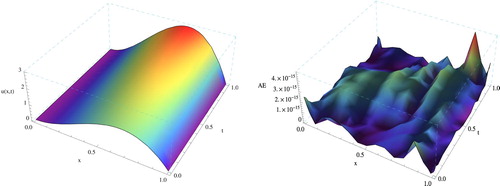
The exact solution is $w(x,t)=10(t+1)x^2(1-x).$ We solve the equation with $\begin{array}{rl}\alpha \left(x\right)& =1-0.5e^{-x},\\ \beta (x,t)& =1.7+0.5e^{-x^2/1000-t/50-1},\\ \gamma (x,t)& =0.7+0.5e^{-x^2/1000-t/50-1}.\end{array}$ The space–time graphs of the approximate solution and the absolute errors (AE) at N=M=4 are shown in Figure 1(left) and (right), respectively.

Figure 1. The space–time graph of approximate solution (left) and AE (right) at N = M = 4 for Example 1.

A comparison of the presented method at N=M=5 with the numerical method proposed in [35] is listed in Table 1.

Table 1. Comparing maximum absolute errors of the proposed method and Implicit Euler approximation (IEA)[35] at t=1 for Example 1.

$x_i$	IEA [35]	Our results $(N=M=4)$
0.1	$2.391\times {10}^{-3}$	$2.220\times {10}^{-15}$
0.2	$5.601\times {10}^{-3}$	$4.440\times {10}^{-15}$
0.3	$9.237\times {10}^{-3}$	$1.231\times {10}^{-15}$
0.4	$1.282\times {10}^{-2}$	$2.775\times {10}^{-15}$
0.5	$1.582\times {10}^{-2}$	$2.220\times {10}^{-15}$
0.6	$1.766\times {10}^{-2}$	$8.881\times {10}^{-15}$
0.7	$1.772\times {10}^{-2}$	$1.665\times {10}^{-15}$
0.8	$1.532\times {10}^{-2}$	$7.216\times {10}^{-15}$
0.9	$9.687\times {10}^{-3}$	$2.220\times {10}^{-15}$

Example 2

Consider the following ST-VO-FADE [35] (32) $\begin{array}{rl}{}_0^{\mathrm{C}}{D}_t^{\alpha \left(x\right)}w(x,t)& =2{}_0^{\mathrm{C}}{D}_x^{\beta (x,t)}w(x,t)\\ & -{}_0^{\mathrm{C}}{D}_x^{\gamma (x,t)}w(x,t)+g(x,t),\\ (x,t)& \in (0,1)\times (0,1],\end{array}$(32) with the initial and boundary conditions: $\begin{array}{rl}w(x,0)& =5x(1-x),x\in (0,1),\\ w(0,t)& =w(1,t)=0,t\in (0,T],\end{array}$ where $\begin{array}{rl}g(x,t)& =\frac{10x^2(1-x)t^{2-\alpha \left(x\right)}}{\mathrm{\Gamma }(3-\alpha (x\left)\right)}\\ & -10(t^2+1)\left[\frac{2x^{2-\beta (x,t)}}{\mathrm{\Gamma }(3-\beta (x,t\left)\right)}-\frac{6x^{3-\beta (x,t)}}{\mathrm{\Gamma }(4-\beta (x,t\left)\right)}\right]\\ & +5(t^2+1)\left[\frac{2x^{2-\gamma (x,t)}}{\mathrm{\Gamma }(3-\gamma (x,t\left)\right)}-\frac{6x^{3-\gamma (x,t)}}{\mathrm{\Gamma }(4-\gamma (x,t\left)\right)}\right].\end{array}$ The exact solution is $w(x,t)=5(t^2+1)x^2(1-x).$

We solve the equation with $\begin{array}{rl}\alpha \left(x\right)& =0.8-0.01\ln \left(5x\right),\\ \beta (x,t)& =1.8+0.01x^2{t}^2,\\ \gamma (x,t)& =0.8+0.01x^2\sin t.\end{array}$

Figure 2 shows the space–time graph of approximate solution (left) and AE (right) of (32(32) $\begin{array}{rl}{}_0^{\mathrm{C}}{D}_t^{\alpha \left(x\right)}w(x,t)& =2{}_0^{\mathrm{C}}{D}_x^{\beta (x,t)}w(x,t)\\ & -{}_0^{\mathrm{C}}{D}_x^{\gamma (x,t)}w(x,t)+g(x,t),\\ (x,t)& \in (0,1)\times (0,1],\end{array}$(32) ) at $N=M=4.$

Figure 2. The space–time graph of approximate solution (left) and AE (right) at N=M=4 for Example 2.

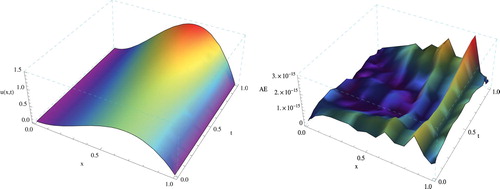
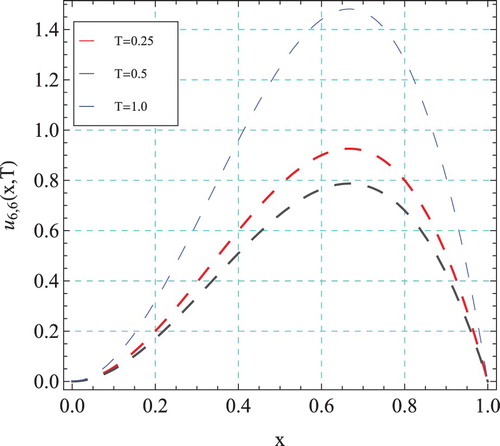
Figure 3 shows the solution behaviour of (32(32) $\begin{array}{rl}{}_0^{\mathrm{C}}{D}_t^{\alpha \left(x\right)}w(x,t)& =2{}_0^{\mathrm{C}}{D}_x^{\beta (x,t)}w(x,t)\\ & -{}_0^{\mathrm{C}}{D}_x^{\gamma (x,t)}w(x,t)+g(x,t),\\ (x,t)& \in (0,1)\times (0,1],\end{array}$(32) ) at $T=0.25,T=0.5$ and T=1 with N=M=6.

Figure 3. The solution behaviour of (32) at T=0:25; T=0:5 and T=1 with N=M=6.

6. Conclusion

In this paper, we have proposed fast and precise algorithm based on shifted Legende collocation technique combined with the associated operational matrices of variable-order fractional derivatives. This algo-rithm was employed for solving the space–time variable-order fractional advection–dispersion model with Caputo time variable fractional derivative and Riemann–Liouville space variable fractional derivatives. This algorithm has the advantage of transforming the problem into the solution of a system of algebraic equations which greatly simplifying the problem. Finally, two numerical examples have been presented to demonstrate the efficiency of the proposed algorithm.

Authors' contributions

The authors have equal contributions to each part of this paper. All the authors read and approved the final manuscript.

Disclosure statement

No potential conflict of interest was reported by the authors.

ORCID

F. Mallawi  http://orcid.org/0000-0002-3434-443X

J. F. Alzaidy  http://orcid.org/0000-0003-2318-8176

R. M. Hafez  http://orcid.org/0000-0001-9533-3171

Correction Statement

This article has been republished with minor changes. These changes do not impact the academic content of the article.

References

- Milici C, Drăgănescu G, Machado JAT. 2019. Introduction to fractional differential equations. Springer.
- Zaky MA. A Legendre collocation method for distributed-order fractional optimal control problems. Nonlinear Dyn. 2018;91:2667–2681. doi: 10.1007/s11071-017-4038-4
- Bhrawy AH, Zaky MA. An improved collocation method for multi-dimensional spacetime variable-order fractional Schrödinger equations. Appl. Numer. Math. 2017;111:197–218. doi: 10.1016/j.apnum.2016.09.009
- Machado JAT, Moghaddam BP. A robust algorithm for nonlinear variable-order fractional control systems with delay. Int. J. Nonlinear Sci. Numer. Simul. 2018;19:231–238. doi: 10.1515/ijnsns-2016-0094
- Zaky MA. An improved tau method for the multi-dimensional fractional Rayleigh–Stokes problem for a heated generalized second grade fluid. Comput. Math. Appl. 2018;75:2243–2258. doi: 10.1016/j.camwa.2017.12.004
- Kilbas AA, Srivastava HM, Trujillo JJ. Theory and applications of fractional differential equations. North-Holl. Math. Stud. 2006;204.
- Bhrawy AH, Zaky MA. Numerical simulation of multi-dimensional distributed-order generalized Schrödinger equations. Nonlinear Dyn. 2018;89:1415–1432. doi: 10.1007/s11071-017-3525-y
- Zaky MA, Machado JAT. On the formulation and numerical simulation of distributed-order fractional optimal control problems. Commun. Nonlinear Sci. Numer. Simul. 2017;52:177–189. doi: 10.1016/j.cnsns.2017.04.026
- Moghaddam BP, Machado JAT, Babaei A. A computationally efficient method for tempered fractional differential equations with application. Comp. Appl. Math. 2018;37:3657–3671. doi: 10.1007/s40314-017-0522-1
- Sohail A, Maqbool K, Ellahi R. Stability analysis for fractional order partial differential equations by means of space spectral time Adams Bashforth Moulton method. Numer. Methods Partial Differ. Equ.2017;34(1):19–29. doi: 10.1002/num.22171
- Bhrawy AH, Zaky MA. A method based on the Jacobi tau approximation for solving multi-term time–space fractional partial differential equations. J. Compt. Phys. 2015;281:876–895. doi: 10.1016/j.jcp.2014.10.060
- Rahmatullah RE, Mohyud-Din ST, Khan U. Exact traveling wave solutions of fractional order Boussinesq-like equations by applying Exp-function method. Results Phys. 2018;8:114–120. doi: 10.1016/j.rinp.2017.11.023
- Khan U, Ellahi R, Khan R, et al. Extracting new solitary wave solutions of Benny Luke equation and Phi-4 equation of fractional order by using (G′/G)-expansion method. Opt. Quantum. Electron. 2017;49:362. doi: 10.1007/s11082-017-1191-4
- Bhrawy AH, Zaky MA. Shifted fractional-order Jacobi orthogonal functions: Application to a system of fractional differential equations. Appl. Math. Model. 2016;40:832–845. doi: 10.1016/j.apm.2015.06.012
- Moghaddam BP, Aghili A. A numerical method for solving linear non-homogenous fractional ordinary differential equation. Appl. Math. Inf. Sc. 2012;6:441–445.
- Bhrawy AH, Zaky MA, Van Gorder RA. A space–time Legendre spectral tau method for the two-sided space–time Caputo fractional diffusion-wave equation. Numer. Algor. 2016;71:151–180. doi: 10.1007/s11075-015-9990-9
- Zaky MA, Doha EH, Machado JAT. A spectral framework for fractional variational problems based on fractional Jacobi functions. Appl. Numer. Math. 2018;132:51–72. doi: 10.1016/j.apnum.2018.05.009
- Bhrawy AH, Zaky MA, Machado JT. Efficient Legendre spectral tau algorithm for solving two-sided space–time Caputo fractional advection–dispersion equation. J. Vib. Control. 2016;22:2053–2068. doi: 10.1177/1077546314566835
- Bhrawy AH, Zaky MA, Baleanu D, et al. A novel spectral approximation for the two-dimensional fractional sub-diffusion problems. Rom. J. Phys. 2015;60:344–359.
- Bhrawy AH, Zaky MA, Machado JAT. Numerical solution of the two-sided space-time fractional telegraph equation via Chebyshev tau approximation. J. Optimiz. Theory App. 2017;174:321–341. doi: 10.1007/s10957-016-0863-8
- Bhrawy AH, Zaky MA. A fractional-order Jacobi tau method for a class of time-fractional PDEs with variable coefficients. Math. Method. Appl. Sci. 2016;39:1765-–1779. doi: 10.1002/mma.3600
- Zaky MA. A Legendre spectral quadrature tau method for the multi-term time-fractional diffusion equations. Comput. Appl. Math.
- Samko SG, Ross B. Integration and differentiation to a variable fractional order. Integr. Transf. Spec. F. 1993;1:277–300. doi: 10.1080/10652469308819027
- Samko SG. Fractional integration and differentiation of variable order. Anal. Math. 1995;21:213–236. doi: 10.1007/BF01911126
- Samko S. Fractional integration and differentiation of variable order: an overview. Nonlinear Dynam. 2013;71:653–662. doi: 10.1007/s11071-012-0485-0
- Zaky MA, Ameen IG, Abdelkawy MA. A new operational matrix based on Jacobi wavelets for a class of variable-order fractional differential equations. Proc. Roman. Academy 2017;18:315–322.
- Diaz G, Coimbra CFM. Nonlinear dynamics and control of a variable order oscillator with application to the van der Pol equation. Nonlinear Dynam. 2009;56:145–157. doi: 10.1007/s11071-008-9385-8
- Zaky MA, Doha EH, Taha TM, et al. New recursive approximations for variable-order fractional operators with applications. Math. Model. Anal. 2018;23:227–239. doi: 10.3846/mma.2018.015
- Lorenzo CF, Hartley TT. Variable order and distributed order fractional operators. Nonlinear Dynam. 2002;29:57–98. doi: 10.1023/A:1016586905654
- Lin R, Liu F, Anh V, et al. Stability and convergence of a new explicit finite-difference approximation for the variable-order nonlinear fractional diffusion equation. Appl. Math. Comput. 2009;212:435–445.
- Sun HG, Chen W, Chen YQ. Variable order fractional differential operators in anomalous diffusion modeling. Physica A Stat. Mech. Appl. 2009;388:4586–4592. doi: 10.1016/j.physa.2009.07.024
- Bhrawy AH, Zaky MA. Highly accurate numerical schemes for multi-dimensional space variable-order fractional Schrödinger equations. Comput. Math. Appl. 2017;73:1100–1117. doi: 10.1016/j.camwa.2016.11.019
- Atangana A, Cloot AH. Stability and convergence of the space fractional variable-order Schrödinger equation. Adv. Differ. Equ. 2013;2013:1–10. doi: 10.1186/1687-1847-2013-1
- Bhrawy AH, Zaky MA. Numerical simulation for two-dimensional variable-order fractional nonlinear cable equation. Nonlinear Dynam. 2015;80:101–116. doi: 10.1007/s11071-014-1854-7
- Zhang H, Liu F, Zhuang P, et al. Numerical analysis of a new space–time variable fractional order advection–dispersion equation. Appl. Math. Comput. 2014;242:541–550.
- Zaky MA, Baleanu D, Alzaidy JF, et al. Operational matrix approach for solving the variable-order nonlinear Galilei invariant advection–diffusion equation. Adv. Differ. Equ. 2018;2018:102. doi: 10.1186/s13662-018-1561-7
- Abdelkawy MA, Zaky MA, Bhrawy AH, et al. Numerical simulation of time variable fractional order mobile–immobile advection–dispersion model. Rom. Rep. Phys. 2015;67:773–791.
- Bhrawy AH, Zaky MA. Numerical algorithm for the variable-order Caputo fractional functional differential equation. Nonlinear Dyn. 2016;85:1815–1823. doi: 10.1007/s11071-016-2797-y
- Moghaddam BP, Mostaghim ZS. A numerical method based on finite difference for solving fractional delay differential equations. J. Taibah Univ. Sci. 2013;7(3):120–127. doi: 10.1016/j.jtusci.2013.07.002
- Ghomanjani F. A new approach for solving fractional differential algebraic equations. J. Taibah Univ. Sci. 2017;11(6):1158–1164. doi: 10.1016/j.jtusci.2017.03.006
- Guezane-Lakoud A, Ramdane S. Existence of solutions for a system of mixed fractional differential equations. J. Taibah Univ. Sci. 2018;12(4):421–426. doi: 10.1080/16583655.2018.1477414
- Yaslan HC, Girgin A. New exact solutions for the conformable space–time fractional KdV, CDG,(2+1)-dimensional CBS and (2+1)-dimensional AKNS equations. J. Taibah Univ. Sci. 2018;13(1):1–8. doi: 10.1080/16583655.2018.1515303
- Sabi'u J, Jibril A, Gadu AM. New exact solution for the (3+1) conformable space–time fractional modified Kortewegde–Vries equations via Sine–Cosine Method. J. Taibah Univ. Sci. 2018;13(1):91–95. doi: 10.1080/16583655.2018.1537642
- Nuruddeen RI, Nass AM. Exact solitary wave solution for the fractional and classical GEW–Burgers equations: an application of Kudryashov method. J. Taibah Univ. Sci. 2018;12(3):309–314. doi: 10.1080/16583655.2018.1469283
- Sun H, Chen W, Chen Y. Variable-order fractional differential operators in anomalous diffusion modeling. Physica A Stat. Mech. Appl. 2009;388:4586–4592. doi: 10.1016/j.physa.2009.07.024
- Fu Z, Chen W, Ling L. Method of approximate particular solutions for constant-and variable-order fractional diffusion models. Eng. Anal. Bound. Elem. 2015;57:37–46. doi: 10.1016/j.enganabound.2014.09.003
- Moghaddam BP, Machado JAT. A computational approach for the solution of a class of variable-order fractional integro-differential equations with weakly singular kernels. Fract. Calc. Appl. Anal. 2017;20:1023–1042.
- Bhrawy AH, Zaky MA, Alzaidy JF. Two shifted Jacobi–Gauss collocation schemes for solving two-dimensional variable-order fractional Rayleigh–Stokes problem. Adv. Differ. Equ. 2016;2016:272. doi: 10.1186/s13662-016-0998-9
- Doha EH, Youssri YH, Zaky MA. Spectral solutions for differential and integral equations with varying coefficients using classical orthogonal polynomials. Bull. Iran. Math. Soc. 2018;8(2):1–29.
- Zaky M, Doha E, Machado JAT. A spectral numerical method for solving distributed-order fractional initial value problems. J. Comput. Nonlinear Dynam. 2018;3:101007.
- Bhrawy AH, Zaky MA, Abdel-Aty M. A fast and precise numerical algorithm for a class of variable-order fractional differential equations. Proc. Rom. Academy. 2017;18:17–24.