Analytical and numerical solutions for the variant Boussinseq equations

Abstract

The principal objective of this paper is to employ the $\exp (-f(\zeta \left)\right)$-expansion and the adaptive moving mesh methods to express the exact travelling wave solutions and the numerical solutions, respectively, for the variant Boussinseq equations. Hyperbolic tangent and cotangent functions are utilized to build the exact solutions. The used numerical method uses the finite differences to discretize the proposed equations. The obtained numerical results are compared with other results obtained using the uniform mesh method. The achieved results show that both solutions match with each other. We also illustrate some 2D and 3D figures to confirm the validity of the numerical approach applied here.

Keywords:

• Variant Boussinseq equations
• adaptive moving mesh equation
• travelling wave solution
• MMPDEs
• monitor function
• $\exp (-f(\eta \left)\right)$-expansion method

AMS Subject Classifications:

• 65N06
• 65N40
• 65N45
• 65N50

1. Introduction

Various complex physical phenomena such as chemical kinematics, plasma physics, chemical physics and optics are investigated using nonlinear evolution equations (NLEEs). Therefore, effective and efficient approaches to construct the travelling wave solutions have attracted a diverse group of experts. Some scientists have developed an extensive variety of techniques to obtain the exact solutions of partial differential equations (PDEs). Some of these methods are the trial function method [1], the inverse scattering transform [2], the Weierstrass elliptic function approach [3], the sine–cosine method [4,5], the F-expansion method [6], the tanh–sech approach [7,8], the modified tanh-function technique [9], Hirota's bilinear method [10,11], the extended tanh-method [12,13], the $\exp (-f(\zeta \left)\right)$-expansion method [14–17], the truncated Painleve expansion [18] and many others (see Refs. [19–29]). It is notable to mention that some of these approaches cannot be sometimes applied to some NLEEs.

Some numerical schemes for solving NLEEs have also been established recently. Among these are the adaptive moving mesh technique [30], the finite element method, the finite differences and the Parabolic Monge–Ampere method [31]. The central purpose of this article is to use the $\exp (-f(\zeta \left)\right)$-expansion and the adaptive moving mesh techniques in extracting the exact and numerical solutions, respectively, for the following variant Boussinseq equations [32,33]: (1) $\begin{array}{rl}& U_t-\alpha U_{xxt}+\frac{1}{2}(U^2{)}_x+G_x=0,\\ & G_t-{\left(UG\right)}_x-\text{β}{U}_{xxx}=0,\end{array}$(1) where U presents the velocity of wave, G denotes the total depth, x is the spatial derivative, t is the temporal derivative, and α and $\text{β}>0$ are arbitrary constants. We also aim to verify that the used numerical technique gives reliable and successful results. Some figures are shown to verify that the behaviours of the exact and numerical solutions are almost the same.

The boundary conditions are graphically discovered from the behaviour of the analytical solution as time increases. The analytical solution becomes fixed at the end points of the physical domain. Hence, the boundary conditions of the solution are constants. This implies that the solution does not change at the end points of the domain and then we observe that $u_x=0$ and $u_{xxx}=0$ as $x\to \pm \mathrm{\infty }$. Hence, the boundary conditions are given by (2) $U_x=U_{xxx}=0\mathrm{a}\mathrm{n}\mathrm{d}{G}_x=0\mathrm{a}\mathrm{t}x\to \pm \mathrm{\infty }.$(2) The rest of this paper is outlined as follows. Section 2 describes the $\exp (-f(\eta \left)\right)$-expansion method which is utilized to express the exact travelling wave solutions. In Section 3, the Hamiltonian system is explained to test the stability of the achieved results. In Section 4, we solve the variant Boussinseq equations and point out some solutions. Section 5.1 is devoted to solve the proposed equation by employing the uniform mesh scheme while Section 5.2 presents the moving mesh approach. The last section concludes this article.

2. The explanation of the $\exp (-f(\eta \left)\right)$-expansion method

A comprehensive explanation to the $\exp (-f(\eta \left)\right)$-expansion approach is clearly given in this section. The description shown here was provided in Refs. [15,16]. This technique is described in few steps illustrated as follows. Assume that (3) $T(v,v_t,v_x,v_{tt},v_{xx},v_{xt},\dots )=0,$(3) where $v\left(\eta \right)=v(x,t)v\left(\eta \right)=v(x,t)$ is an unknown function and TT is a polynomial of v.v., is a PDE with two independent variables x and t. In order to reduce Equation (3(3) $T(v,v_t,v_x,v_{tt},v_{xx},v_{xt},\dots )=0,$(3) ) to an ordinary differential equation (ODE), we introduce the transformation (4) $\eta =x\pm wt,v(x,t)=g\left(\eta \right).$(4) Expanding the derivatives in Equation (3(3) $T(v,v_t,v_x,v_{tt},v_{xx},v_{xt},\dots )=0,$(3) ) using the chain rule leads to the ODE (5) $R(g,g_{\eta },g_{\eta \eta },g_{\eta \eta \eta },\dots )=0,$(5) where R is a polynomial in $v\left(\eta \right)$ and (6) $g_{\eta }=\frac{\mathrm{d}g}{\mathrm{d}\eta },g_{\eta \eta }=\frac{{\mathrm{d}}^{2}g}{\mathrm{d}{\eta }^2},\dots$(6) According to this technique, the solution of Equation (5(5) $R(g,g_{\eta },g_{\eta \eta },g_{\eta \eta \eta },\dots )=0,$(5) ) is given in the form (7) $g\left(\eta \right)=\sum _{m=0}^n{a}_m{\mathrm{e}}^{-mf\left(\eta \right)},$(7) where the constants $a_0,a_1,a_2,\dots ,a_n$ will be calculated later. Furthermore, $a_n\ne 0,$ and $f=f\left(\eta \right)$ fulfils the equation (8) $f_{\eta }={\mathrm{e}}^{-f\left(\eta \right)}+\mu {\mathrm{e}}^{f\left(\eta \right)}+\lambda .$(8) We now turn to present various cases for the solutions of Equation (8(8) $f_{\eta }={\mathrm{e}}^{-f\left(\eta \right)}+\mu {\mathrm{e}}^{f\left(\eta \right)}+\lambda .$(8) ).

• If ${\lambda }^2-4\mu >0,\mu \ne 0,$ then

  1. $\begin{array}{rl}& 1.f\left(\eta \right)\\ & =\ln \left(\frac{-\sqrt{({\lambda }^2-4\mu )}\tanh \left(\right(\sqrt{({\lambda }^2-4\mu )}/2\left)\right(\eta +k\left)\right)-\lambda }{2\mu }\right),\\ & 2.f\left(\eta \right)\\ & =\ln \left(\frac{-\sqrt{({\lambda }^2-4\mu )}\coth \left(\right(\sqrt{({\lambda }^2-4\mu )}/2\left)\right(\eta +k\left)\right)-\lambda }{2\mu }\right).\end{array}$

• If ${\lambda }^2-4\mu <0,\mu \ne 0,$ then

  1. $\begin{array}{rl}& 1.f\left(\eta \right)\\ & =\ln \left(\frac{\sqrt{(4\mu -{\lambda }^2)}\tan \left(\right(\sqrt{(4\mu -{\lambda }^2)}/2\left)\right(\eta +k\left)\right)-\lambda }{2\mu }\right),\\ & 2.f\left(\eta \right)\\ & =\ln \left(\frac{\sqrt{(4\mu -{\lambda }^2)}\cot \left(\right(\sqrt{(4\mu -{\lambda }^2)}/2\left)\right(\eta +k\left)\right)-\lambda }{2\mu }\right).\end{array}$

• If ${\lambda }^2-4\mu >0,\mu =0,\lambda \ne 0,$ then (9) $f\left(\eta \right)=-\ln \left(\frac{\lambda }{\exp \left(\lambda \right(\eta +k\left)\right)-1}\right).$(9)

• If ${\lambda }^2-4\mu =0,\mu \ne 0,\lambda \ne 0,$ then (10) $f\left(\eta \right)=\ln \left(-\frac{2\left(\lambda \right(\eta +k)+2}{{\lambda }^2(\eta +k))}\right).$(10)

• If ${\lambda }^2-4\mu =0,\mu =0,\lambda =0,$ then (11) $f\left(\eta \right)=\ln \left(\eta +k\right),$(11)

where k is an arbitrary constant. The constants $\mu ,\lambda ,w,$ and $a_n$ are evaluated later. When we insert Equation (7(7) $g\left(\eta \right)=\sum _{m=0}^n{a}_m{\mathrm{e}}^{-mf\left(\eta \right)},$(7) ) into Equation (5(5) $R(g,g_{\eta },g_{\eta \eta },g_{\eta \eta \eta },\dots )=0,$(5) ) and equate the coefficients of the same order of $\exp (-f(\eta \left)\right),$ we end up with an algebraic system that can be simply solved (using some software such as Maple or Mathematica) to evaluate the values of $\mu ,\lambda ,w,$ and $a_n.$ Substituting $\mu ,\lambda ,w,$ and $a_n$ into Equations (7(7) $g\left(\eta \right)=\sum _{m=0}^n{a}_m{\mathrm{e}}^{-mf\left(\eta \right)},$(7) ) and (8(8) $f_{\eta }={\mathrm{e}}^{-f\left(\eta \right)}+\mu {\mathrm{e}}^{f\left(\eta \right)}+\lambda .$(8) ) shows the solution of Equation (3(3) $T(v,v_t,v_x,v_{tt},v_{xx},v_{xt},\dots )=0,$(3) ).

3. Stability analysis

The stability of the achieved exact solutions is tested using the Hamiltonian system expressed as (12) $\begin{array}{rl}{\rho }_1& ={\int }_{-\mathrm{\infty }}^{\mathrm{\infty }}\frac{1}{2}{U}^2\left(\eta \right)\mathrm{d}\eta ,\\ {\rho }_2& =\frac{1}{2}{\int }_{-\mathrm{\infty }}^{\mathrm{\infty }}\frac{1}{2}{G}^2\left(\eta \right)\mathrm{d}\eta ,\end{array}$(12) where ${\rho }_i\left(w\right)$ indicates the momentum and U and G are the obtained solutions of the system (1(1) $\begin{array}{rl}& U_t-\alpha U_{xxt}+\frac{1}{2}(U^2{)}_x+G_x=0,\\ & G_t-{\left(UG\right)}_x-\text{β}{U}_{xxx}=0,\end{array}$(1) ). The sufficient condition for the stability can be illustrated as follows: (13) $\frac{\mathrm{\partial }{\rho }_i}{\mathrm{\partial }w}>0\mathrm{\forall }i=1,2.$(13)

4. The exact solution of the variant Boussinseq equations

This section concerns with determining the travelling wave solutions of the variant Boussinseq equations. The variant Boussinseq equations [32,33] are given by (14) $\begin{array}{rl}{U}_t-\alpha U_{xxt}+U{U}_x+G_x& =0,\\ G_t-{\left(UG\right)}_x-\text{β}{U}_{xxx}& =0,\end{array}$(14) where α and β are arbitrary constants and $\text{β}>0.$ We begin with introducing the transformation (15) $\eta =x-wt,U(x,t)=u\left(\eta \right)\mathrm{a}\mathrm{n}\mathrm{d}G(x,t)=g\left(\eta \right)$(15) to alter system (14(14) $\begin{array}{rl}{U}_t-\alpha U_{xxt}+U{U}_x+G_x& =0,\\ G_t-{\left(UG\right)}_x-\text{β}{U}_{xxx}& =0,\end{array}$(14) ) into the ODEs (16) $\begin{array}{rl}-w{u}_{\eta }+w\alpha u_{\eta \eta \eta }+\frac{1}{2}(u^2{)}_{\eta }+g_{\eta }& =0,\\ -w{g}_{\eta }-{\left(ug\right)}_{\eta }-\text{β}{u}_{\eta \eta \eta }& =0.\end{array}$(16) The ODEs in system (16(16) $\begin{array}{rl}-w{u}_{\eta }+w\alpha u_{\eta \eta \eta }+\frac{1}{2}(u^2{)}_{\eta }+g_{\eta }& =0,\\ -w{g}_{\eta }-{\left(ug\right)}_{\eta }-\text{β}{u}_{\eta \eta \eta }& =0.\end{array}$(16) ) are now integrated with respect to η once to yield (17) $\begin{array}{rl}-wu+w\alpha u_{\eta \eta }+\frac{1}{2}\left(u^2\right)+g& =p_1,\\ -wg-ug-\text{β}{u}_{\eta \eta }& =p_2,\end{array}$(17) where $p_1$ and $p_2$ are the integration constants. Balancing the highest order $u_{\eta \eta }$ and non-linear term $u^2$ in the first equation of (17(17) $\begin{array}{rl}-wu+w\alpha u_{\eta \eta }+\frac{1}{2}\left(u^2\right)+g& =p_1,\\ -wg-ug-\text{β}{u}_{\eta \eta }& =p_2,\end{array}$(17) ) and the terms $u_{\eta \eta }$ and $ug$ in the second equation, we have 2N = N + 2 and 2N = N + M which leads to N = 2 and $M=2.$ Thus, the solutions are given by (18) $\begin{array}{rl}u\left(\eta \right)& =\sum _{k=0}^N{a}_k{\mathrm{e}}^{-kf\left(\eta \right)},\\ g\left(\eta \right)& =\sum _{k=0}^M{b}_k{\mathrm{e}}^{-kf\left(\eta \right)}.\end{array}$(18) And then, (19) $\begin{array}{rl}u\left(\eta \right)& =a_0+a_1{\mathrm{e}}^{-f\left(\eta \right)}+a_2{\mathrm{e}}^{-2f\left(\eta \right)},\\ g\left(\eta \right)& =b_0+b_1{\mathrm{e}}^{-f\left(\eta \right)}+b_2{\mathrm{e}}^{-2f\left(\eta \right)}.\end{array}$(19) The values of the constants $a_0,a_1,a_2,b_0,b_1$ and $b_2$ are shown later. The first equation in system (19(19) $\begin{array}{rl}u\left(\eta \right)& =a_0+a_1{\mathrm{e}}^{-f\left(\eta \right)}+a_2{\mathrm{e}}^{-2f\left(\eta \right)},\\ g\left(\eta \right)& =b_0+b_1{\mathrm{e}}^{-f\left(\eta \right)}+b_2{\mathrm{e}}^{-2f\left(\eta \right)}.\end{array}$(19) ) is now inserted into the first equation in system (17(17) $\begin{array}{rl}-wu+w\alpha u_{\eta \eta }+\frac{1}{2}\left(u^2\right)+g& =p_1,\\ -wg-ug-\text{β}{u}_{\eta \eta }& =p_2,\end{array}$(17) ) and the coefficients of ${\mathrm{e}}^{-kf\left(\eta \right)},k\ge 0,$ are equalized to zero to introduce the following algebraic system: (20) $\begin{array}{rl}& \frac{a_0^2}{2}-a_{0}w+a_1\alpha \lambda \mu w+2a_2\alpha {\mu }^{2}w+b_0-p_1=0,\\ & \frac{1}{2}{a}_2^2+6a_2\alpha w=0,\\ & a_1{a}_2+2a_1\alpha w+10a_2\alpha \lambda w=0,\\ & a_0{a}_2+\frac{1}{2}{a}_1^2+3a_1\alpha \lambda w+4a_2\alpha {\lambda }^{2}w+8a_2\alpha \mu w\\ & -a_{2}w+b_2=0,\\ & a_0{a}_1+a_1\alpha {\lambda }^{2}w+2a_1\alpha \mu w-a_{1}w\\ & +6a_2\alpha \lambda \mu w+b_1=0.\end{array}$(20) Similarly, when we substitute the second equation in system (19(19) $\begin{array}{rl}u\left(\eta \right)& =a_0+a_1{\mathrm{e}}^{-f\left(\eta \right)}+a_2{\mathrm{e}}^{-2f\left(\eta \right)},\\ g\left(\eta \right)& =b_0+b_1{\mathrm{e}}^{-f\left(\eta \right)}+b_2{\mathrm{e}}^{-2f\left(\eta \right)}.\end{array}$(19) ) into the second equation in system (17(17) $\begin{array}{rl}-wu+w\alpha u_{\eta \eta }+\frac{1}{2}\left(u^2\right)+g& =p_1,\\ -wg-ug-\text{β}{u}_{\eta \eta }& =p_2,\end{array}$(17) ) and equate the coefficients of ${\mathrm{e}}^{-mf\left(\eta \right)},m\ge 0,$ to zero, we end up with (21) $\begin{array}{rl}& -a_0{b}_0-a_1\text{β}\lambda \mu -2a_2\text{β}{\mu }^2-b_{0}w-p_2=0,\\ & -a_2{b}_2-6a_2\text{β}=0,\\ & -a_1{b}_2-2a_1\text{β}-a_2{b}_1-10a_2\text{β}\lambda =0,\\ & -a_0{b}_2-a_1{b}_1-3a_1\text{β}\lambda -a_2{b}_0-4a_2\text{β}{\lambda }^2\\ & -8a_2\text{β}\mu -b_{2}w=0,\\ & -a_0{b}_1-a_1{b}_0-a_1\text{β}{\lambda }^2-2a_1\text{β}\mu \\ & -6a_2\text{β}\lambda \mu -b_{1}w=0.\end{array}$(21) Solving the previous algebraic systems (by Maple or Mathematica) gives

• Case I (22) $\begin{array}{rl}{a}_0& =\frac{-2{\alpha }^2{\lambda }^2{w}^2-16{\alpha }^2\mu w^2+2\alpha w^2-\text{β}}{2\alpha w},\\ a_1& =-12\alpha \lambda w,a_2=-12\alpha w,\\ b_0& =\frac{-2{\alpha }^2\text{β}{\lambda }^2{w}^2-16{\alpha }^2\text{β}\mu w^2-4\alpha \text{β}{w}^2+{\text{β}}^2}{4{\alpha }^2{w}^2},\\ b_1& =-6\text{β}\lambda ,b_2=-6\text{β},\\ p_1& =\frac{\begin{array}{c}4{\alpha }^4{\lambda }^4{w}^4-32{\alpha }^4{\lambda }^2\mu w^4+64{\alpha }^4{\mu }^2{w}^4\\ -4{\alpha }^2{w}^4-8\alpha \text{β}{w}^2+3{\text{β}}^2\end{array}}{8{\alpha }^2{w}^2},\\ p_2& =\frac{\begin{array}{c}-4{\alpha }^4\text{β}{\lambda }^4{w}^4+32{\alpha }^4\text{β}{\lambda }^2\mu w^4-64{\alpha }^4\text{β}{\mu }^2{w}^4\\ +16{\alpha }^2\text{β}{w}^4-8\alpha {\text{β}}^2{w}^2+{\text{β}}^3\end{array}}{8{\alpha }^3{w}^3}.\end{array}$(22)

• Case II (23) $\begin{array}{rl}{a}_0& =-\sqrt{\text{β}}\lambda ,a_1=-2\sqrt{\text{β}},a_2=0,\\ b_0& =-2\text{β}\mu ,\\ b_1& =-2\text{β}\lambda ,b_2=-2\text{β},\\ p_1& =0,p_2=0.\end{array}$(23)

Putting λ and μ, so that ${\lambda }^2-4\mu >0,$ gives

• From Case I, the exact solutions are given by

(24) $\begin{array}{rl}& \begin{array}{rl}u\left(\eta \right)& =a_0-\frac{2\mu a_1}{\sqrt{({\lambda }^2-4\mu )}\tanh \left(\frac{1}{2}\sqrt{{\lambda }^2-4\mu }(\eta +k)\right)+\lambda }\\ & +\frac{4{\mu }^2{a}_2}{{\left(\sqrt{({\lambda }^2-4\mu )}\tanh \left(\frac{1}{2}\sqrt{{\lambda }^2-4\mu }(\eta +k)\right)+\lambda \right)}^2},\\ g\left(\eta \right)& =b_0-\frac{2\mu b_1}{\sqrt{({\lambda }^2-4\mu )}\tanh \left(\frac{1}{2}\sqrt{{\lambda }^2-4\mu }(\eta +k)\right)+\lambda }\\ & +\frac{4{\mu }^2{b}_2}{{\left(\sqrt{({\lambda }^2-4\mu )}\tanh \left(\frac{1}{2}\sqrt{{\lambda }^2-4\mu }(\eta +k)\right)+\lambda \right)}^2},\end{array}\end{array}$(24) (25) $\begin{array}{rl}& \begin{array}{rl}u\left(\eta \right)& =a_0-\frac{2\mu a_1}{\sqrt{({\lambda }^2-4\mu )}\coth \left(\frac{1}{2}\sqrt{{\lambda }^2-4\mu }(\eta +k)\right)+\lambda }\\ & +\frac{4{\mu }^2{a}_2}{{\left(\sqrt{({\lambda }^2-4\mu )}\coth \left(\frac{1}{2}\sqrt{{\lambda }^2-4\mu }(\eta +k)\right)+\lambda \right)}^2},\\ g\left(\eta \right)& =b_0-\frac{2\mu b_1}{\sqrt{({\lambda }^2-4\mu )}\coth \left(\frac{1}{2}\sqrt{{\lambda }^2-4\mu }(\eta +k)\right)+\lambda }\\ & +\frac{4{\mu }^2{b}_2}{{\left(\sqrt{({\lambda }^2-4\mu )}\coth \left(\frac{1}{2}\sqrt{{\lambda }^2-4\mu }(\eta +k)\right)+\lambda \right)}^2}.\end{array}\end{array}$(25)

• From Case II

(26) $\begin{array}{rl}u\left(\eta \right)& =-\sqrt{\text{β}}\lambda +2\sqrt{\text{β}}\frac{2\mu }{\sqrt{({\lambda }^2-4\mu )}\tanh \left(\frac{1}{2}\sqrt{{\lambda }^2-4\mu }(\eta +k)\right)+\lambda },\\ g\left(\eta \right)& =-2\text{β}\mu +\frac{4\mu \text{β}\lambda }{\sqrt{({\lambda }^2-4\mu )}\tanh \left(\frac{1}{2}\sqrt{{\lambda }^2-4\mu }(\eta +k)\right)+\lambda }\\ & -\frac{8{\mu }^2\text{β}}{{\left(\sqrt{({\lambda }^2-4\mu )}\tanh \left(\frac{1}{2}\sqrt{{\lambda }^2-4\mu }(\eta +k)\right)+\lambda \right)}^2},\end{array}$(26) (27) $\begin{array}{rl}u\left(\eta \right)& =-\sqrt{\text{β}}\lambda +2\sqrt{\text{β}}\frac{2\mu }{\sqrt{({\lambda }^2-4\mu )}\coth \left(\frac{1}{2}\sqrt{{\lambda }^2-4\mu }(\eta +k)\right)+\lambda },\\ g\left(\eta \right)& =-2\text{β}\mu +\frac{4\mu \text{β}\lambda }{\sqrt{({\lambda }^2-4\mu )}\coth \left(\frac{1}{2}\sqrt{{\lambda }^2-4\mu }(\eta +k)\right)+\lambda }\\ & -\frac{8{\mu }^2\text{β}}{{\left(\sqrt{({\lambda }^2-4\mu )}\coth \left(\frac{1}{2}\sqrt{{\lambda }^2-4\mu }(\eta +k)\right)+\lambda \right)}^2}.\end{array}$(27) Setting λ and μ, so that ${\lambda }^2-4\mu <0,$ yields

• From Case I, the exact solutions are illustrated as follows:

(28) $\begin{array}{rl}u\left(\eta \right)& =a_0+a_1\frac{2\mu }{\sqrt{({\lambda }^2-4\mu )}\tan \left(\frac{1}{2}\sqrt{{\lambda }^2-4\mu }(\eta +k)\right)-\lambda }\\ & +a_2\frac{4{\mu }^2}{{\left(\sqrt{({\lambda }^2-4\mu )}\tan \left(\frac{1}{2}\sqrt{{\lambda }^2-4\mu }(\eta +k)\right)-\lambda \right)}^2},\\ g\left(\eta \right)& =b_0+b_1\frac{2\mu }{\sqrt{({\lambda }^2-4\mu )}\tan \left(\frac{1}{2}\sqrt{{\lambda }^2-4\mu }(\eta +k)\right)-\lambda }\\ & +b_2\frac{4{\mu }^2}{{\left(\sqrt{({\lambda }^2-4\mu )}\tan \left(\frac{1}{2}\sqrt{{\lambda }^2-4\mu }(\eta +k)\right)-\lambda \right)}^2},\end{array}$(28) (29) $\begin{array}{rl}u\left(\eta \right)& =a_0+a_1\frac{2\mu }{\sqrt{({\lambda }^2-4\mu )}\cot \left(\frac{1}{2}\sqrt{{\lambda }^2-4\mu }(\eta +k)\right)-\lambda }\\ & +a_2\frac{4{\mu }^2}{{\left(\sqrt{({\lambda }^2-4\mu )}\cot \left(\frac{1}{2}\sqrt{{\lambda }^2-4\mu }(\eta +k)\right)-\lambda \right)}^2},\\ g\left(\eta \right)& =b_0+b_1\frac{2\mu }{\sqrt{({\lambda }^2-4\mu )}\cot \left(\frac{1}{2}\sqrt{{\lambda }^2-4\mu }(\eta +k)\right)-\lambda }\\ & +b_2\frac{4{\mu }^2}{{\left(\sqrt{({\lambda }^2-4\mu )}\cot \left(\frac{1}{2}\sqrt{{\lambda }^2-4\mu }(\eta +k)\right)-\lambda \right)}^2}.\end{array}$(29)

• From Case II, we have

(30) $\begin{array}{rl}u\left(\eta \right)& =-\sqrt{\text{β}}\lambda -2\sqrt{\text{β}}\frac{2\mu }{\sqrt{({\lambda }^2-4\mu )}\tan \left(\frac{1}{2}\sqrt{{\lambda }^2-4\mu }(\eta +k)\right)-\lambda },\\ g\left(\eta \right)& =-2\text{β}\mu -\frac{4\mu \text{β}\lambda }{\sqrt{({\lambda }^2-4\mu )}\tan \left(\frac{1}{2}\sqrt{{\lambda }^2-4\mu }(\eta +k)\right)-\lambda }\\ & -\frac{8{\mu }^2\text{β}\lambda }{{\left(\sqrt{({\lambda }^2-4\mu )}\tan \left(\frac{1}{2}\sqrt{{\lambda }^2-4\mu }(\eta +k)\right)-\lambda \right)}^2},\end{array}$(30) (31) $\begin{array}{rl}u\left(\eta \right)& =-\sqrt{\text{β}}\lambda -2\sqrt{\text{β}}\frac{2\mu }{\sqrt{({\lambda }^2-4\mu )}\cot \left(\frac{1}{2}\sqrt{{\lambda }^2-4\mu }(\eta +k)\right)-\lambda },\\ g\left(\eta \right)& =-2\text{β}\mu -\frac{4\mu \text{β}\lambda }{\sqrt{({\lambda }^2-4\mu )}\cot \left(\frac{1}{2}\sqrt{{\lambda }^2-4\mu }(\eta +k)\right)-\lambda }\\ & -\frac{8{\mu }^2\text{β}}{{\left(\sqrt{({\lambda }^2-4\mu )}\cot \left(\frac{1}{2}\sqrt{{\lambda }^2-4\mu }(\eta +k)\right)-\lambda \right)}^2}.\end{array}$(31) When ${\lambda }^2-4\mu =0,\mu \ne 0,\lambda \ne 0,$ we can observe that

• From Case I, we obtain (32) $\begin{array}{rl}u\left(\eta \right)& =\frac{-2{\alpha }^2{\lambda }^2{w}^2-16{\alpha }^2\mu w^2+2\alpha w^2-\text{β}}{2\alpha w}\\ & +\frac{12\alpha w(\eta +k){\lambda }^3}{2(1+\eta \lambda +k\lambda )}-\frac{12\alpha w(\eta +k{)}^2{\lambda }^4}{4(1+\eta \lambda +k\lambda {)}^2},\\ g\left(\eta \right)& =\frac{-2{\alpha }^2\text{β}{\lambda }^2{w}^2-16{\alpha }^2\text{β}\mu w^2-4\alpha \text{β}{w}^2+{\text{β}}^2}{4{\alpha }^2{w}^2}\\ & -\frac{6\text{β}(\eta +k){\lambda }^3}{2(1+\eta \lambda +k\lambda )}-\frac{6\text{β}(\eta +k{)}^2{\lambda }^4}{4(1+\eta \lambda +k\lambda {)}^2}.\end{array}$(32)

• From Case II, we have (33) $\begin{array}{rl}u\left(\eta \right)& =-\sqrt{\text{β}}\lambda +\frac{2\sqrt{\text{β}}(\eta +k){\lambda }^2}{2(1+\eta \lambda +k\lambda )},\\ g\left(\eta \right)& =-2\text{β}\mu -\frac{2\text{β}(\eta +k){\lambda }^3}{2(1+\eta \lambda +k\lambda )}\\ & -\frac{2\text{β}(\eta +k{)}^2{\lambda }^4}{4(1+\eta \lambda +k\lambda {)}^2}.\end{array}$(33)

When ${\lambda }^2-4\mu =0,\mu =0,\lambda =0,$ we observe that

• From Case I, we obtain (34) $\begin{array}{rl}u\left(\eta \right)& =\frac{-2{\alpha }^2{\lambda }^2{w}^2-16{\alpha }^2\mu w^2+2\alpha w^2-\text{β}}{2\alpha w}\\ & -\frac{12\alpha \lambda w}{\left(\eta +k\right)}-\frac{12\alpha w}{{\left(\eta +k\right)}^2},\\ g\left(\eta \right)& =\frac{-2{\alpha }^2\text{β}{\lambda }^2{w}^2-16{\alpha }^2\text{β}\mu w^2-4\alpha \text{β}{w}^2+{\text{β}}^2}{4{\alpha }^2{w}^2}\\ & -\frac{6\text{β}\lambda }{\left(\eta +k\right)}-\frac{6\text{β}}{{\left(\eta +k\right)}^2}.\end{array}$(34)

• From Case II, we have (35) $\begin{array}{rl}u\left(\eta \right)& =-\sqrt{\text{β}}\lambda -\frac{2\sqrt{\text{β}}}{\left(\eta +k\right)},\\ g\left(\eta \right)& =-2\text{β}\mu -\frac{2\text{β}\lambda }{\left(\eta +k\right)}-\frac{2\text{β}}{{\left(\eta +k\right)}^2},\end{array}$(35)

where $\eta =x-wt.$ To investigate the numerical results of Equation (14(14) $\begin{array}{rl}{U}_t-\alpha U_{xxt}+U{U}_x+G_x& =0,\\ G_t-{\left(UG\right)}_x-\text{β}{U}_{xxx}& =0,\end{array}$(14) ), we semi-discretize the spatial derivatives utilizing the centred finite differences (second-order accurate) and the temporal derivative is kept continuous. Therefore, the main equation has been converted to a system of ODEs solved utilizing the method of lines with the initial condition from Equation (24(24) $\begin{array}{rl}& \begin{array}{rl}u\left(\eta \right)& =a_0-\frac{2\mu a_1}{\sqrt{({\lambda }^2-4\mu )}\tanh \left(\frac{1}{2}\sqrt{{\lambda }^2-4\mu }(\eta +k)\right)+\lambda }\\ & +\frac{4{\mu }^2{a}_2}{{\left(\sqrt{({\lambda }^2-4\mu )}\tanh \left(\frac{1}{2}\sqrt{{\lambda }^2-4\mu }(\eta +k)\right)+\lambda \right)}^2},\\ g\left(\eta \right)& =b_0-\frac{2\mu b_1}{\sqrt{({\lambda }^2-4\mu )}\tanh \left(\frac{1}{2}\sqrt{{\lambda }^2-4\mu }(\eta +k)\right)+\lambda }\\ & +\frac{4{\mu }^2{b}_2}{{\left(\sqrt{({\lambda }^2-4\mu )}\tanh \left(\frac{1}{2}\sqrt{{\lambda }^2-4\mu }(\eta +k)\right)+\lambda \right)}^2},\end{array}\end{array}$(24) ) at t = 0 and the boundary conditions from Equation (2(2) $U_x=U_{xxx}=0\mathrm{a}\mathrm{n}\mathrm{d}{G}_x=0\mathrm{a}\mathrm{t}x\to \pm \mathrm{\infty }.$(2) ). In the following section, we use the MATLAB ODE solver (ode15i), which is a variable order implicit time-stepping method based on the numerical differentiation formulas (NDFs), to solve the system.

5. Numerical results

This section is devoted to extract the numerical solutions of Equation (14(14) $\begin{array}{rl}{U}_t-\alpha U_{xxt}+U{U}_x+G_x& =0,\\ G_t-{\left(UG\right)}_x-\text{β}{U}_{xxx}& =0,\end{array}$(14) ) using uniform and adaptive moving mesh methods. To employ these approaches, we first introduce a variable V as follows: (36) $V=U-\alpha U_{xx}.$(36) Hence, Equation (14(14) $\begin{array}{rl}{U}_t-\alpha U_{xxt}+U{U}_x+G_x& =0,\\ G_t-{\left(UG\right)}_x-\text{β}{U}_{xxx}& =0,\end{array}$(14) ) is converted to (37) $\begin{array}{rl}& V_t+\frac{1}{2}(U^2{)}_x+G_x=0,\\ & G_t-{\left(UG\right)}_x-\text{β}{U}_{xxx}=0.\end{array}$(37) The used boundary conditions are given by Equation(2(2) $U_x=U_{xxx}=0\mathrm{a}\mathrm{n}\mathrm{d}{G}_x=0\mathrm{a}\mathrm{t}x\to \pm \mathrm{\infty }.$(2) ).

5.1. Numerical solutions using a uniform mesh

A uniform mesh approach, on a physical domain $[0,L]$, is now employed to deal with the numerical results of Equation (37(37) $\begin{array}{rl}& V_t+\frac{1}{2}(U^2{)}_x+G_x=0,\\ & G_t-{\left(UG\right)}_x-\text{β}{U}_{xxx}=0.\end{array}$(37) ). The used domain is split into N subintervals $[x_j,x_{j+1}]$ with fixed step size $\mathrm{\Delta }x=L/N$ such that $x_n=n\mathrm{\Delta }x\mathrm{\forall }{x}_n\in [0,L],n=0,1,2,\dots ,N,$ where $\mathrm{\Delta }x$ presents a uniform width of each subinterval. The discretization of the spatial derivatives is accomplished by applying the finite difference operators. Note that the temporal differentiation is kept continuous. Thus, the discretization of Equation (37(37) $\begin{array}{rl}& V_t+\frac{1}{2}(U^2{)}_x+G_x=0,\\ & G_t-{\left(UG\right)}_x-\text{β}{U}_{xxx}=0.\end{array}$(37) ) is given by (38) $\begin{array}{rl}& V_{n,t}+\frac{U_{n+1/2}^2-U_{n-1/2}^2}{2\mathrm{\Delta }x}+\frac{G_{n+1/2}-G_{n-1/2}}{\mathrm{\Delta }x}=0,\\ & G_{n,t}-\frac{(UG{)}_{n+1/2}-(UG{)}_{n-1/2}}{\mathrm{\Delta }x}-\text{β}{U}_{n,xxx}=0,\end{array}$(38) where (39) $\begin{array}{rl}{U}_{n+1/2}& =\frac{U_{n+1}+U_n}{2},\\ (UG{)}_{n+1/2}& =\frac{(UG{)}_{n+1}+(UG{)}_n}{2},\\ G_{n+1/2}& =\frac{G_{n+1}+G_n}{2},\\ U_{n,xxx}& =\frac{1}{\mathrm{\Delta }{x}^3}\left(U_{n+2}-3U_{n+1}+3U_n-U_{n-1}\right),\end{array}$(39) and $n=0,1,2,\dots ,N.$ The associated boundary values of Equation (2(2) $U_x=U_{xxx}=0\mathrm{a}\mathrm{n}\mathrm{d}{G}_x=0\mathrm{a}\mathrm{t}x\to \pm \mathrm{\infty }.$(2) ) are $u_{t,0}=u_{t,N}=0$ and the initial condition is generated by letting t = 0 in Equation (24(24) $\begin{array}{rl}& \begin{array}{rl}u\left(\eta \right)& =a_0-\frac{2\mu a_1}{\sqrt{({\lambda }^2-4\mu )}\tanh \left(\frac{1}{2}\sqrt{{\lambda }^2-4\mu }(\eta +k)\right)+\lambda }\\ & +\frac{4{\mu }^2{a}_2}{{\left(\sqrt{({\lambda }^2-4\mu )}\tanh \left(\frac{1}{2}\sqrt{{\lambda }^2-4\mu }(\eta +k)\right)+\lambda \right)}^2},\\ g\left(\eta \right)& =b_0-\frac{2\mu b_1}{\sqrt{({\lambda }^2-4\mu )}\tanh \left(\frac{1}{2}\sqrt{{\lambda }^2-4\mu }(\eta +k)\right)+\lambda }\\ & +\frac{4{\mu }^2{b}_2}{{\left(\sqrt{({\lambda }^2-4\mu )}\tanh \left(\frac{1}{2}\sqrt{{\lambda }^2-4\mu }(\eta +k)\right)+\lambda \right)}^2},\end{array}\end{array}$(24) ).

5.2. Numerical solutions using an adaptive mesh

We now turn to employ the adaptive mesh method to obtain the numerical results of Equation (37(37) $\begin{array}{rl}& V_t+\frac{1}{2}(U^2{)}_x+G_x=0,\\ & G_t-{\left(UG\right)}_x-\text{β}{U}_{xxx}=0.\end{array}$(37) ). Start by transforming the physical domain $[0,L]$ to the computational domain provided by $[0,1]$ such that $x=x(\zeta ,t):[0,1]\to [0,L],t>0,$ to execute the proposed numerical technique. Using the physical coordinate x and computational coordinate ζ gives (40) $U=U(x,t),G=G(x,t)\mathrm{w}\mathrm{h}\mathrm{e}\mathrm{r}\mathrm{e}x=x(\zeta ,t).$(40) We now divide the physical domain to equal sub-intervals as follows: $x_0<x_1<x_2<\cdots <x_n<\cdots <x_N,$ where $x_n\left(\zeta \right)=x({\zeta }_n,t),n=0,1,\dots ,N,$ with $x_0=0,x_N=L$. Additionally, the nodes are presented by ${\zeta }_n=n\left(1/\right(N-1\left)\right),n=0,1,\dots ,N.$ Applying the chain rule for Equation (37(37) $\begin{array}{rl}& V_t+\frac{1}{2}(U^2{)}_x+G_x=0,\\ & G_t-{\left(UG\right)}_x-\text{β}{U}_{xxx}=0.\end{array}$(37) ) yields (41) $\begin{array}{rl}& \dot{V}-\left(\frac{U_{\zeta }}{x_{\zeta }}\right)\dot{x}=-\left(\frac{1}{x_{\zeta }}(U^2/2+G{)}_{\zeta }\right),\\ & \dot{G}-\left(\frac{G_{\zeta }}{x_{\zeta }}\right)\dot{x}=\frac{1}{x_{\zeta }}{\left(UG+\text{β}{U}_{xx}\right)}_{\zeta },\\ & U_{xx}=\frac{1}{x_{\zeta }}{\left(\frac{U_{\zeta }}{x_{\zeta }}\right)}_{\zeta }.\end{array}$(41) It is worth pointing out that the error and the convergence of the adaptive moving scheme for different MMPDEs (and their parameters) and various monitor functions are deeply considered to obtain the new mesh. We found that all these mesh equations give the same results. Consequently, we here utilize the most commonly used one which is MMPDE5 [30,34–36] given by (42) $\mathbf{M}\mathbf{M}\mathbf{P}\mathbf{D}\mathbf{E}\mathbf{5}\mathbf{:}\tau \left(I-\gamma {\mathrm{\partial }}_{\zeta \zeta }\right)\dot{x}={\left(\varphi x_{\zeta }\right)}_{\zeta },$(42) where the smoothing operator $(I-\gamma {\mathrm{\partial }}_{\zeta \zeta })$ is important to make the computation easier and faster [37,38], $\tau \in (0,1)$ is a relaxation parameter, $\gamma =\sqrt{max\left(\varphi \right)}$ is selected by Budd et al. [31] and Walsh [37] and $\varphi (U,G,x)$ is called a monitor function. The monitor function depends on the solutions' changes and controls the movement of the mesh so that it increases the number of the mesh points where the solution has significant variations and fewer points elsewhere. Here, we use an exceptional monitor function given by (43) $\varphi (U,G,x)=\sqrt{1+r_1(U-U(1){)}^2+r_2(G-G\left(1\right){)}^2},$(43) where $r_1$ and $r_2$ are constants. In this section, we fix the parameter values by $r_1=10,r_2=10,k=-6,$ $\lambda =2.1,\mu ={10}^{-1},\alpha ={10}^{-1},\text{β}=2\times {10}^{-1},$ w = 1 and $\tau ={10}^{-3}.$ The semi-discretizations of MMPDE5 (Equation(42(42) $\mathbf{M}\mathbf{M}\mathbf{P}\mathbf{D}\mathbf{E}\mathbf{5}\mathbf{:}\tau \left(I-\gamma {\mathrm{\partial }}_{\zeta \zeta }\right)\dot{x}={\left(\varphi x_{\zeta }\right)}_{\zeta },$(42) )) and system equation (41(41) $\begin{array}{rl}& \dot{V}-\left(\frac{U_{\zeta }}{x_{\zeta }}\right)\dot{x}=-\left(\frac{1}{x_{\zeta }}(U^2/2+G{)}_{\zeta }\right),\\ & \dot{G}-\left(\frac{G_{\zeta }}{x_{\zeta }}\right)\dot{x}=\frac{1}{x_{\zeta }}{\left(UG+\text{β}{U}_{xx}\right)}_{\zeta },\\ & U_{xx}=\frac{1}{x_{\zeta }}{\left(\frac{U_{\zeta }}{x_{\zeta }}\right)}_{\zeta }.\end{array}$(41) ) are shown as (44) $\begin{array}{rl}& \mathrm{\Delta }{\zeta }^2\tau {\dot{x}}_i-\tau \left({\dot{x}}_{i+1}-2{\dot{x}}_i+{\dot{x}}_{i-1}\right)\\ & =\left[{\varphi }_{i+1/2}\left(x_{i+1}-x_i\right)-{\varphi }_{i-1/2}\left(x_i-x_{i-1}\right)\right].\end{array}$(44) We use here the average value of the monitor function so that ${\varphi }_{i+1/2}=({\varphi }_{i+1}+{\varphi }_i)/2$ and ${\varphi }_{i-1/2}=({\varphi }_i+{\varphi }_{i-1})/2.$ (45) $\begin{array}{rl}& {\dot{V}}_i=\left(\frac{U_{i+1}-U_{i-1}}{x_{i+1}-x_{i-1}}\right)\\ & \dot{x}-\left(\frac{(U^2/2+G{)}_{i+1}-(U^2/2+G{)}_{i-1}}{x_{i+1}-x_{i-1}}\right),\\ & \dot{G}=\left(\frac{G_{i+1}-G_{i-1}}{x_{i+1}-x_{i-1}}\right)\\ & \dot{x}+\left(\frac{(UG+\text{β}{U}_{xx}{)}_{i+1}-(UG+\text{β}{U}_{xx}{)}_{i-1}}{x_{i+1}-x_{i-1}}\right),\\ & U_{xx,i}=\frac{2}{x_{i+1}-x_{i-1}}\left(\frac{U_{i+1}-U_i}{x_{i+1}-x_i}-\frac{U_i-U_{i-1}}{x_i-x_{i-1}}\right),\\ & i=1,3,\dots ,N-1.\end{array}$(45) The initial condition is taken by (46) $x_j=j\frac{L}{N-1},j=0,1,\dots ,N.$(46) The boundary conditions of the equations given in systems (44(44) $\begin{array}{rl}& \mathrm{\Delta }{\zeta }^2\tau {\dot{x}}_i-\tau \left({\dot{x}}_{i+1}-2{\dot{x}}_i+{\dot{x}}_{i-1}\right)\\ & =\left[{\varphi }_{i+1/2}\left(x_{i+1}-x_i\right)-{\varphi }_{i-1/2}\left(x_i-x_{i-1}\right)\right].\end{array}$(44) ) and (45(45) $\begin{array}{rl}& {\dot{V}}_i=\left(\frac{U_{i+1}-U_{i-1}}{x_{i+1}-x_{i-1}}\right)\\ & \dot{x}-\left(\frac{(U^2/2+G{)}_{i+1}-(U^2/2+G{)}_{i-1}}{x_{i+1}-x_{i-1}}\right),\\ & \dot{G}=\left(\frac{G_{i+1}-G_{i-1}}{x_{i+1}-x_{i-1}}\right)\\ & \dot{x}+\left(\frac{(UG+\text{β}{U}_{xx}{)}_{i+1}-(UG+\text{β}{U}_{xx}{)}_{i-1}}{x_{i+1}-x_{i-1}}\right),\\ & U_{xx,i}=\frac{2}{x_{i+1}-x_{i-1}}\left(\frac{U_{i+1}-U_i}{x_{i+1}-x_i}-\frac{U_i-U_{i-1}}{x_i-x_{i-1}}\right),\\ & i=1,3,\dots ,N-1.\end{array}$(45) ) are converted to (47) ${\dot{x}}_0={\dot{x}}_N=0,\dot{\phantom{a}}{U}_0={\dot{U}}_N=0\mathrm{a}\mathrm{n}\mathrm{d}{\dot{G}}_0={\dot{G}}_N=0.$(47) Some fictitious points are required to compute the boundaries of $U_{xx},G_x$ and $U_x$ (48) $\begin{array}{rl}{U}_{-1}& =U_1,U_{N+1}=U_{N-1}\mathrm{\forall }t\in [0,T_e],\\ G_{-1}& =G_1,U_{xx,-1}=U_{xx,1},\\ G_{N+1}& =G_{N-1},U_{xx,N+1}=U_{xx,N-1}.\end{array}$(48)

The sufficient conditions for the stability (Equations(12(12) $\begin{array}{rl}{\rho }_1& ={\int }_{-\mathrm{\infty }}^{\mathrm{\infty }}\frac{1}{2}{U}^2\left(\eta \right)\mathrm{d}\eta ,\\ {\rho }_2& =\frac{1}{2}{\int }_{-\mathrm{\infty }}^{\mathrm{\infty }}\frac{1}{2}{G}^2\left(\eta \right)\mathrm{d}\eta ,\end{array}$(12) ) and (13(13) $\frac{\mathrm{\partial }{\rho }_i}{\mathrm{\partial }w}>0\mathrm{\forall }i=1,2.$(13) )) are employed, and then we discover that all of the achieved solutions are stable in the interval $[0,20].$ Figure 1(a,b) presents the evolution time of the exact and numerical results and Figure 1(c) presents the mesh behaviour taken at $t=0\to 10$ with fixed number of points $N=1000.$ Figure 2 shows the exact and numerical results for both U and G at t = 5 and $N=1000.$ All of the parameter values are fixed, as mentioned above. Figure 3(a,b) illustrates the behaviour of the travelling waves for both the exact and numerical solutions. We note that, from all of the above figures, the exact and the numerical results are almost identical. The insets in Figure 2 show the steep front regions which take more points than elsewhere. Therefore, the results appear almost equal in these regions for both $U(x,t)$ and $G(x,t)$.Table 1 illustrates $L_2$ error and CPU time taken to reach $t=5$ for the adaptive moving and uniform mesh (using MMPDE5 (42(42) $\mathbf{M}\mathbf{M}\mathbf{P}\mathbf{D}\mathbf{E}\mathbf{5}\mathbf{:}\tau \left(I-\gamma {\mathrm{\partial }}_{\zeta \zeta }\right)\dot{x}={\left(\varphi x_{\zeta }\right)}_{\zeta },$(42) ) and the modified monitor function (43(43) $\varphi (U,G,x)=\sqrt{1+r_1(U-U(1){)}^2+r_2(G-G\left(1\right){)}^2},$(43) )) approaches. The numerical results are obtained at $t=5.$ Figure 4 summaries the error columns in Table 1 (solid blue line for the adaptive mesh scheme and solid red line for the uniform mesh scheme). It can be easily observed that the error for the adaptive moving mesh is much smaller and is accomplished utilizing less number of nodes compared to the uniform mesh method. However, regarding the CPU time consumed, the uniform mesh scheme consumes less time to reach t = 5 compared to the adaptive moving mesh technique for the same number of points. This can be attributed to the additional adaptive functions which are required to be simultaneously resolved along with the PDE. As the number of points increases, the error for the adaptive moving scheme sharply decreases with a slight increase in the CPU time. Therefore, it can be definitely concluded that the adaptive moving mesh technique is more computationally effective than the uniform mesh method.

Figure 1. (a) and (b) The time evolution for the exact and numerical solutions, respectively. (c) The movement of the mesh $x(\xi ,t)$. The results are obtained for $0\le t\le 10$ and $N=1000.$

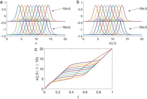
Figure 2. The comparison between the exact solutions evaluated by (24(24) $\begin{array}{rl}& \begin{array}{rl}u\left(\eta \right)& =a_0-\frac{2\mu a_1}{\sqrt{({\lambda }^2-4\mu )}\tanh \left(\frac{1}{2}\sqrt{{\lambda }^2-4\mu }(\eta +k)\right)+\lambda }\\ & +\frac{4{\mu }^2{a}_2}{{\left(\sqrt{({\lambda }^2-4\mu )}\tanh \left(\frac{1}{2}\sqrt{{\lambda }^2-4\mu }(\eta +k)\right)+\lambda \right)}^2},\\ g\left(\eta \right)& =b_0-\frac{2\mu b_1}{\sqrt{({\lambda }^2-4\mu )}\tanh \left(\frac{1}{2}\sqrt{{\lambda }^2-4\mu }(\eta +k)\right)+\lambda }\\ & +\frac{4{\mu }^2{b}_2}{{\left(\sqrt{({\lambda }^2-4\mu )}\tanh \left(\frac{1}{2}\sqrt{{\lambda }^2-4\mu }(\eta +k)\right)+\lambda \right)}^2},\end{array}\end{array}$(24) ) and the numerical results obtained by solving the system (45(45) $\begin{array}{rl}& {\dot{V}}_i=\left(\frac{U_{i+1}-U_{i-1}}{x_{i+1}-x_{i-1}}\right)\\ & \dot{x}-\left(\frac{(U^2/2+G{)}_{i+1}-(U^2/2+G{)}_{i-1}}{x_{i+1}-x_{i-1}}\right),\\ & \dot{G}=\left(\frac{G_{i+1}-G_{i-1}}{x_{i+1}-x_{i-1}}\right)\\ & \dot{x}+\left(\frac{(UG+\text{β}{U}_{xx}{)}_{i+1}-(UG+\text{β}{U}_{xx}{)}_{i-1}}{x_{i+1}-x_{i-1}}\right),\\ & U_{xx,i}=\frac{2}{x_{i+1}-x_{i-1}}\left(\frac{U_{i+1}-U_i}{x_{i+1}-x_i}-\frac{U_i-U_{i-1}}{x_i-x_{i-1}}\right),\\ & i=1,3,\dots ,N-1.\end{array}$(45) ) for U and G at t = 5 and $N=1000.$

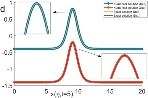
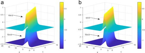
Figure 3. (a) 3D plot for the exact solution (24(24) $\begin{array}{rl}& \begin{array}{rl}u\left(\eta \right)& =a_0-\frac{2\mu a_1}{\sqrt{({\lambda }^2-4\mu )}\tanh \left(\frac{1}{2}\sqrt{{\lambda }^2-4\mu }(\eta +k)\right)+\lambda }\\ & +\frac{4{\mu }^2{a}_2}{{\left(\sqrt{({\lambda }^2-4\mu )}\tanh \left(\frac{1}{2}\sqrt{{\lambda }^2-4\mu }(\eta +k)\right)+\lambda \right)}^2},\\ g\left(\eta \right)& =b_0-\frac{2\mu b_1}{\sqrt{({\lambda }^2-4\mu )}\tanh \left(\frac{1}{2}\sqrt{{\lambda }^2-4\mu }(\eta +k)\right)+\lambda }\\ & +\frac{4{\mu }^2{b}_2}{{\left(\sqrt{({\lambda }^2-4\mu )}\tanh \left(\frac{1}{2}\sqrt{{\lambda }^2-4\mu }(\eta +k)\right)+\lambda \right)}^2},\end{array}\end{array}$(24) ) and (b) the numerical results of the system (45(45) $\begin{array}{rl}& {\dot{V}}_i=\left(\frac{U_{i+1}-U_{i-1}}{x_{i+1}-x_{i-1}}\right)\\ & \dot{x}-\left(\frac{(U^2/2+G{)}_{i+1}-(U^2/2+G{)}_{i-1}}{x_{i+1}-x_{i-1}}\right),\\ & \dot{G}=\left(\frac{G_{i+1}-G_{i-1}}{x_{i+1}-x_{i-1}}\right)\\ & \dot{x}+\left(\frac{(UG+\text{β}{U}_{xx}{)}_{i+1}-(UG+\text{β}{U}_{xx}{)}_{i-1}}{x_{i+1}-x_{i-1}}\right),\\ & U_{xx,i}=\frac{2}{x_{i+1}-x_{i-1}}\left(\frac{U_{i+1}-U_i}{x_{i+1}-x_i}-\frac{U_i-U_{i-1}}{x_i-x_{i-1}}\right),\\ & i=1,3,\dots ,N-1.\end{array}$(45) ) of U and G. The results are taken at time which increases from 0 to 10, and $N=1000.$

6. Conclusions

The discussion of this article concentrates on constructing the travelling wave solutions and the numerical solutions of the variant Boussinseq equations by applying the $\exp (-f(\eta \left)\right)$-expansion and the adaptive mesh approaches, respectively. The given 2D and 3D figures show that the solutions agree and coincide together. As can be seen in Table 1, $L_2$ error for the adaptive mesh scheme vanishes for a very small $\mathrm{\Delta }x.$ The error for the uniform mesh scheme is found larger than the error for the adaptive mesh scheme. The achieved results have been compared to each other and found that the performance of the adaptive scheme is effective and appropriate to be utilized in high-order PDEs.

Figure 4. $L_2$ error obtained of U for both the uniform and adaptive mesh methods against the number of mesh points N. The parameter values are taken by $r_1=10,r_2=10,k=-6,$ $\lambda =2.1,\mu ={10}^{-1},\alpha ={10}^{-1},\text{β}=2\times {10}^{-1},$ w = 1 and $\tau ={10}^{-3}.$

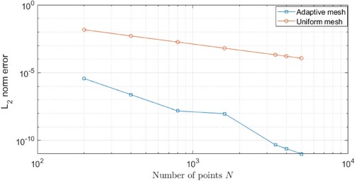
Table 1. $L_2$ error and CPU time taken to arrive t = 5 for both the adaptive and uniform mesh (using MMPDE5 (42(42) $\mathbf{M}\mathbf{M}\mathbf{P}\mathbf{D}\mathbf{E}\mathbf{5}\mathbf{:}\tau \left(I-\gamma {\mathrm{\partial }}_{\zeta \zeta }\right)\dot{x}={\left(\varphi x_{\zeta }\right)}_{\zeta },$(42) ) and the modified monitor function (43(43) $\varphi (U,G,x)=\sqrt{1+r_1(U-U(1){)}^2+r_2(G-G\left(1\right){)}^2},$(43) )) schemes.

	$L_2$ error measured by $U(x,t)$		CPU
N	Adaptive mesh	Uniform mesh	Adaptive mesh	Uniform mesh
200	$3.705\times {10}^{-6}$	$1.460\times {10}^{-2}$	$1.3\times {10}^{-2}$ s	$7.3\times {10}^{-3}$ s
400	$2.400\times {10}^{-7}$	$5.140\times {10}^{-3}$	$2.6\times {10}^{-2}$ s	$1.3\times {10}^{-2}$ s
800	$1.518\times {10}^{-8}$	$1.820\times {10}^{-3}$	$5.5\times {10}^{-2}$ s	$6.5\times {10}^{-2}$ s
1600	$9.540\times {10}^{-9}$	$6.400\times {10}^{-4}$	$2.1\times {10}^{-1}$ s	$7.0\times {10}^{-2}$ s
3400	$4.715\times {10}^{-11}$	$2.080\times {10}^{-4}$	2.1 s	$2.2\times {10}^{-1}$ s
4000	$2.490\times {10}^{-11}$	$1.631\times {10}^{-4}$	2.72 s	$4.0\times {10}^{-1}$ s
5000	$1.040\times {10}^{-11}$	$1.168\times {10}^{-4}$	6.1 s	$5.3\times {10}^{-1}$ s

Disclosure statement

No potential conflict of interest was reported by the author(s).

References

- Inc M, Evans DJ. On traveling wave solutions of some nonlinear evolution equations. Int J Comput Math. 2004;81:191–202. DOI:10.1080/00207160310001603307.
- Ablowitz MJ, Clarkson PA. Solitons, non-linear evolution equations and inverse scattering transformCambridge University Press; 1991. DOI:10.1017/CBO9780511623998.
- Chow KW. A class of exact periodic solutions of nonlinear envelope equation. J Math Phys. 1995;36:4125–4137. DOI:10.1063/1.530951.
- Wazwaz AM. Exact solutions to the double sinh-Gordon equation by the tanh method and a variable separated ODE. method. Comput Math Appl. 2005;50:1685–1696. DOI:10.1016/j.camwa.2005.05.010.
- Wazwaz AM. A sine–cosine method for handling nonlinear wave equations. Math Comput Model. 2004;40:499–508. DOI:10.1016/j.mcm.2003.12.010.
- Zhang JL, Wang ML, Wang YM. The improved F-expansion method and its applications. Phys Lett A. 2006;350:103–109. DOI:10.1016/j.physleta.2005.10.099.
- Malflieta W, Hereman W. The tanh method: exact solutions of nonlinear evolution and wave equations. Phys Scr. 1996;54:563–568. DOI:10.1088/0031-8949/54/6/003.
- Wazwaz AM. The tanh method for travelling wave solutions of nonlinear equations. Appl Math Comput. 2004;154:714–723. DOI:10.1016/S0096-3003(03)00745-8.
- Zhang B, Zhang X, Dai C. Discussions on localized structures based on equivalent solution with different forms of breaking soliton model. Nonlinear Dyn. 2017;87:2385–2393. DOI:10.1007/s11071-016-3197-z.
- Hirota R. Exact envelope soliton solutions of a nonlinear wave equation. J Math Phys. 1973;14:805–810. DOI:10.1063/1.1666399.
- Hirota R, Satsuma J. Soliton solution of a coupled KdV equation. Phys Lett A. 1981;85:407–408. DOI:10.1016/0375-9601.
- Fan E. Extended tanh-function method and its applications to nonlinear equations. Phys Lett A. 2000;277:212–218. DOI:10.1016/S0375-9601(00)00725-8.
- Wazwaz AM. The extended tanh method for abundant solitary wave solutions of nonlinear wave equations. Appl Math Comput. 2007;187:1131–1142. DOI:10.1016/j.amc.2006.09.013.
- Alam MN, Tunc C. An analytical method for solving exact solutions of the nonlinear Bogoyavlenskii equation and the nonlinear diffusive predator–prey system. Alex Eng J. 2016;55:1855–1865. DOI:10.1016/j.aej.2016.04.024.
- Khan K, Akbar MA. Application of Exp(-phi(xi))-expansion method to find the exact solutions of modified Benjamin–Bona–Mahony equation. World Appl Sci J. 2013;24:1373–1377. DOI:10.5829/idosi.wasj.2013.24.10.1130.
- Khan K, Akbar MA. Exact traveling wave solutions of Kadomtsev–Petviashvili equation. J Egyptian Math Soc. 2015;23:278–281. DOI:10.1016/j.joems.2014.03.010.
- Mahmoud A, Hassan S. New-exact-solutions-for-the-Maccari-system. J Phys Math. 2018;9(1):264), DOI:10.4172/2090-0902.1000264.
- Wang ML, Li XZ. Extended F-expansion and periodic wave solutions for the generalized Zakharov equations. Phys Lett A. 2005;343:48–54. DOI:10.1016/j.physleta.2005.05.085.
- Fan E, Zhang H. A note on the homogeneous balance method. Phys Lett A. 1998;246:403–406. DOI:10.1016/S0375-9601.
- Abdelrahman MAE, Sohaly M, Alharbi AR. The new exact solutions for the deterministic and stochastic (2 + 1)-dimensional equations in natural sciences. J Taibah Univ Sci. 2019;13:834–843. DOI:10.1080/16583655.2019.1644832.
- Alam MN, Tunç C. Constructions of the optical solitons and other solitons to the conformable fractional Zakharov–Kuznetsov equation with power law nonlinearity. J Taibah Univ Sci. 2019;14(1):94–100. DOI:10.1080/16583655.2019.1708542.
- Shahida N, Tunç C. Resolution of coincident factors in altering the flow dynamics of an MHD elastoviscous fluid past an unbounded upright channel. J Taibah Univ Sci. 2019;13(1):1022–1034. DOI:10.1080/16583655.2019.1678897.
- Dai C, Fan Y, Wang Y. Three-dimensional optical solitons formed by the balance between different-order nonlinearities and high-order dispersion/diffraction in parity-time symmetric potentials. Nonlinear Dyn. 2019;98:489–499. DOI:10.1007/s11071-019-05206-z.
- Dai C, Wang Y, Fan Y. Interactions between exotic multi-valued solitons of the (2+1)-dimensional Korteweg–de Vries equation describing shallow water wave. Appl Math Mode. 2020;80:506–515. DOI:10.1016/j.apm.2019.11.056.
- Kong L, Liu J, Jin D. Soliton dynamics in the three-spine α -helical protein with inhomogeneous effect. Nonlinear Dyn. 2017;87(1):83–92. DOI:10.1007/s11071-016-3027-3.
- Alharbi AR, Almatrafi MB, Abdelrahman MAE. The extended Jacobian elliptic function expansion approach to the generalized fifth order KdV equation. J Phys Math. 2019;10(4):310). https://www.omicsonline.org/open-access/an-extended-jacobian-elliptic-function-expansion-approach-to-the-generalized-fifth-order-kdv-equation-110076.html.
- Alharbi AR, Almatrafi MB. Numerical investigation of the dispersive long wave equation using an adaptive moving mesh method and its stability. Results Phys. 2020;16: 102870. DOI:10.1016/j.rinp.2019.102870.
- Alharbi AR, Almatrafi MB. Riccati–Bernoulli sub-ODE approach on the partial differential equations and applications. Int J Math Comput Sci. 2020;15(1):367–388. http://ijmcs.future-in-tech.net/15.1/R-Almatrafi.pdf.
- Ding D, Jin D, Dai C. Analytical solutions of differential-difference Sine-Gordon equation. Thermal Sci. 2017;21(4):1701–1705. DOI:10.2298/TSCI160809056D.
- Huang W, Russell RD. The adaptive moving mesh methods. Springer; 2011. DOI:10.1007/978-1-4419-7916-2.
- Budd CJ, Huang W, Russell RD. Adaptivity with moving grids. Acta Numer. 2009;18:111–241. DOI:10.1017/S0962492906400015.
- Zhang HQ. Extended Jacobi elliptic function expansion method and its applications. Commun Nonlinear Sci Numer Simul. 2007;12:627–635. DOI:10.1155/2012/896748.
- Zayed EME, Al-Joudi S. An Improved (G'/G)-expansion Method for Solving Nonlinear PDEs in Mathematical Physics. ICNAAM AIP Conf Proc. 2010;1281:2220–2224. DOI:10.1063/1.3498416.
- Alharbi AR, Naire S. An adaptive moving mesh method for thin film flow equations with surface tension. J Comput Appl Math. 2017;319(4):365–384. DOI:10.1016/j.cam.2017.01.019.
- Alharbi AR, Shailesh N. An adaptive moving mesh method for two-dimensional thin film flow equations with surface tension. J Comput Appl Math. 2019;356:219–230. DOI:10.1016/j.cam.2019.02.010.
- Alharbi AR. 2016. Numerical solution of thin-film flow equations using adaptive moving mesh methods [Ph.D. thesis]. Keele: Keele University.
- Walsh E. Moving mesh methods for problems in meteorology [PhD thesis]. Bath: University of Bath; 2010.
- Ceniceros HD, Hou TY. An efficient dynamically adaptive mesh for potentially singular solutions. J Comput Phys. 2001;172(2):609–639. DOI:10.1006/jcph.2001.6844.