Comprehensive analysis on copper-iron (II, III)/oxide-engine oil Casson nanofluid flowing and thermal features in parabolic trough solar collector

Abstract

Heat is absorbed from radiations of the sun by a solar collector, concentrated, and then transmitted to an active nanofluid. The flow of Casson nanofluid is utilized in Parabolic Trough Solar Collector (PTSC) in the present analysis over an infinite and porous sheet. Ordinary differential equations are derived in nonlinear form and solved using suitable similarity transformation reducing into boundary conditions. Keller box method was employed to solve the system of ODEs. Results for nanofluids of Copper-engine oil (Cu-EO), as well as Iron (II, III) oxide-engine oil (Fe₃O₄-EO), were examined and detailed. With the help of the induced magnetic factor, the rate of heat transfer decreased while the parameter of skin resistance increased prominently. While using Cu/Fe₃O₄-EO as base fluid, the rate of heat transfer is an important factor. Total enhancement in the thermal efficiency of Cu-EO on Fe₃O₄-EO has a minimum value of 2.7% while the maximum value is 18.5%.

KEYWORDS:

• Solar energy
• Parabolic Trough Solar Collector
• steady flow
• Casson-nanofluid
• variable thermal conductivity
• Keller box method

1. Introduction

Solar energy is a luminous light as well as the heat coming from the sun, which is made useful utilizing different ever-growing technologies. Solar thermal energy, solar heating, solar architecture, photovoltaic, artificial photosynthesis, and molten salt power plants are a few of its forms. It is a capital source of energy that can be made renewable using different technologies. It is mainly the best source to generate electricity for having a great amount of magnitude [1]. Mainly there are two types of solar energy. One is photovoltaic and the other is solar thermal energy. Photovoltaic energy is formed utilizing photovoltaic solar technology that changes solar energy directly into electricity with the help of solar panels that are made using cells of semiconductors. Later is obtained with the help of solar thermal technology. Here, heat from the sun's radiation is absorbed to either directly convert it into electricity or first into mechanical energy and then into electricity [2]. The importance of solar energy is undeniable, just like its benefits. As many businessmen and homeowners are using solar panels. As solar energy does not need any fossil fuels, so it is a good choice for the environment. As solar energy has no contribution to global warming, so it is preferable. As fossil fuels usually run out that's why conventional electricity is found expensive. Solar energy is a reliable source of energy as well as cost-effective. Installing solar energy panels needs money just once, but using conventional electricity is an expensive and ongoing way as its rates are always rising. Solar energy saves much of your money. According to a recent census, the solar energy sector employed 17% more jobs than the overall economy of a country. As solar energy is purely sun’ energy, so there is no need for grid stations. It helps in energy independence [3]. Solar energy has wide applications. Solar distillation, solar water heating, solar cooking, solar heating of buildings, solar furnaces, solar greenhouses, solar thermal power production, and solar electric power generation are a few of its applications [4].

Long and parabolic-shaped mirrors are used to make a linear and concentrating system, along with a receiver tube placed in the focal axis of the parabola, called a parabolic trough collector (PTC). The receiver tube is used to focus the DNI where HTF is absorbing the solar energy. It is the most mature technology [5]. Applications of PTSC involve cooling, heat driven-refrigeration, and heat demand having low temperature along with high rates of consumption, like space heating, swimming pool heating, and domestic hot water [6]. Nanofluids are suspended nano-sized particles that make collisions in the fluid. Nanofluids are used in a fluid to increase heat capacity and heat transfer abilities. Major applications of nanofluids focus on their main type known as nano-suspension. Recently, nanotechnology is playing a major role in the process of heat transfer and energy applications. Its best application is the production of nanofluids having high thermal conductivity. When nanofluids are mixed in the working fluids, base fluids show huge enhancement in their thermal features [7]. Sheikhpour et. al [8] worked on nanofluids in the medical field to check the role of nanofluids. In the biomedical field, its applications involve drug delivery systems, antibiotic activities, and imaging. Drug delivery and differential diagnosis are targeted through applying magnetic systems of nanofluids. & Das [9] reviewed the various methods to prepare the nanofluids, their uses, and surfactants used to stabilize them. Wang & De Leon [10] focused on new and recent applications of nanofluids by improving the controllable features of heat transfer and other prominent characteristics. Using Nickel Ferrite (NiFe₂O₄) nanofluid and U-tube as new base fluid and absorbent respectively, Dehaj et. al [11] investigated the efficiency of PTSC. Nickel Ferrite nanofluid was developed using a two-step procedure. Alashkar & Gadalla [12] used Ag/Therminol nanofluids in PTSC to check their impact on the efficiency of the power plant that was based on PTSC. Pressure drops and coefficient of convective heat transfer were observed under the impact of nanofluids. They also studied the pumping power using various shapes and sizes of nanoparticles.

There are mainly two types of slip conditions. One is the no-slip boundary condition while the other is the slip boundary condition. In the no-slip boundary condition, also known as the no-velocity-offset boundary condition, a fluid layer having direct contact with the boundary has the same speed as the velocity of the boundary. As there is no relative motion between the two so no slip. In slip boundary conditions, there is a discontinuity between boundary and layer, hence slip exists. Case with slip boundary condition is rare in the field of microfluidics [13]. A boundary condition that is related to the convection heating on the surface and can be achieved through the balance of surface energy is called the convection boundary condition. Haq et al. [14] used an incompressible and viscous fluid flow having ramped wall temperature and heat transfer, to explore the effect of slip condition of the wall. Sayed et al. [15] used the convective boundary conditions and leaning and asymmetric tunnel to investigate the peristaltic transfer of hyperbolic tangent nanofluid. Srinivasacharya & Himabindu [16] utilized the porous tunnel to represent the influence of velocity slip and convective heating on the flow of an incompressible fluid having micro-polar generation. Acharya et al. [17] made an analysis using a permeable stretching surface to explore the impact of second order slip mechanism on the flow of nanofluid.

Casson fluid is such a shear-thinning fluid that is considered to have zero viscosity at the infinite shear rate but infinite viscosity at zero shear rates. Its examples include honey, jelly, soap, concentrated fruit juices, tomato sauce, as well as human blood. Casson fluid model is for non-Newtonian fluids. Existence of fibrinogen, protein, and globulin in aqueous plasma results in the formation of a chain-like arrangement by red blood cells of a human being, called rouleaux. If it operates as a plastic solid, there can be a presence of yield stress which can be recognized as the constant yield stress of the Casson fluid [18]. The flow of the blood at a low rate of shear that is passing through the small tubes is described by Casson fluid model. The non-linear stretching surface was utilized by Mukjopadhyay [19] to examine the impacts of heat transfer along with the flow of Casson fluid. MHD flow of Casson fluid was used to study the Dufour and Soret impacts over a stretching sheet [20,21]. Chamkha and Aly [22] used Dufour and Soret effects along with various chemical reactions to analyze the mass and heat transfer in the polar fluid flow over a stretching and porous sheet. Non-linear set of Casson constitutive equations was derived by Casson [23] depicting the various characteristics of polymers. Non-Newtonian nanofluids have many technological and industrial applications. Some of them are biological solutions, asphalt, paints, glues, tars, and melts of polymers. Recently, they are of great interest in every field [24–26]. Sivaraj & Banerjee [27] analyzed recent features of non-Newtonian nanofluids to give guidelines to future researchers. Few research works to be noted from the literature are [28–33]. Abdelsalam & Bhatti [34] used the effect of hall currents and magnetic field to examine the motion of non-Newtonian nanofluid that has peristaltic and unsteady nature. They also utilized chemical reactions along with ion slip. Niu et al. [35] used a micro-tube to study the heat transfer and slip flow of non-Newtonian nanofluid, theoretically. Flow features were described using power-law rheology.

Thermal conductivity is the measurability of some substance that how much it can conduct the heat in itself. So it is mainly dependent on temperature. In gasses, the thermal conductivity increases with an increase in temperature but in solid, thermal conductivity decreases. As every material has its thermal conductivity so it is variable significantly. Variable thermal conductivity is a linear function of temperature. Hayat et al. [36] used a stretchable sheet of changeable thickness to analyze the stagnation point flow with temperature depending on thermal conductivity. They utilized Catteneo-Christov theory, chemical reaction, and double stratification. Abel & Mahesha [37] worked on MHD boundary layer flow along with features of heat transfer of non-Newtonian and viscoelastic fluid. They utilized a flat surface under the effect of non-uniform heat source and thermal radiation as well as linear velocity. They also utilized variable thermal conductivity. Sharma & Singh [38] investigated the influence of heat source and variable thermal conductivity on a viscous and incompressible fluid flow with electrical conductance properties. They used variable free stream and uniform transverse magnetic field close to the stagnation point of stretchable surface that is non-conducting. Chiu [39] employed variable thermal conductivity to evaluate the optimal length and competency of the convective and rectangular fin with the help of Adomian decomposition technique. He also determined the distribution of temperature in the fin. Usman et al. [40] used 3D stretching surface to evaluate the prominent effects of time-dependent thermal conductivity and non-linear thermal radiation on the Cu–Al₂O₃–water hybrid nanofluid flow with rotation. They considered the effect of magnetic fields and bouncy forces. Lahmar et al. [41] worked on the special case between two parallel plates when there is the existence of an inclined magnetic field and thermal conductivity is dependent on temperature. They examine the heat transfer and flow of unsteady and squeezing (Fe₃O₄–water) nanofluid. Irfan et al. [42] used a bidirectional stretched sheet to obtain a relation of 3D Carreau nanofluid flow having force convection and unsteadiness. Variable thermal conductivity was employed to inspect heat transfer in Carreau nanofluid.

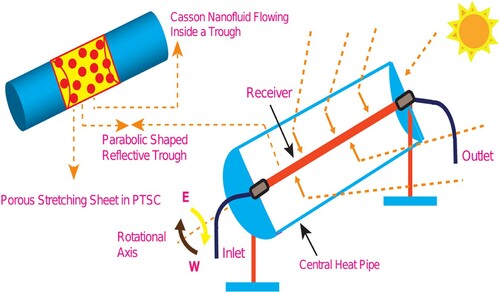
Mahian et al. [43] considered various flow systems and geometries to examine the contribution of heat transfer and flow in nanofluids on entropy generation. Bosca & Pop [44] used the stability of orthogonal shear of the surface to study the heat transfer and flow in hybrid nanofluids that are induced with an absorbable power-law stretching sheet. Selimefendigil & Öztop [45] studied the impact of a partially curved and porous sheet on features of entropy generation and thermal management inside the hybrid nanofluid-filled cavity with the help of finite volume method. Yang et al. [46] proposed a model for thermal conductivity using heat conduction analysis of finite length of cylindrical nanoparticles in the liquid. They obtained the radial and axial thermal conductivities. Figure 1 represents a parabolic trough, solar collector.

Figure 1. PTSC.

Literature mentioned above reveals that researchers had focused on thermal efficiency and entropy analysis of solar collectors and as such, nanofluid application becomes crucial in the analysis of PTSC. Hence, the authors would like to investigate the nanofluid in PTSC and the present research study focuses on entropy formation in PTSC in a MHD Casson nanofluid flow on an infinite horizontal surface. In this work, two tested nanofluid Cu-engine oil and Iron (II, III) oxide-engine oil operational fluids have been used to analyze the thermal efficiency of PTSC. Also, the effect of performance parameters, such as Nusselt number, skin resistance feature, Reynolds number, and Brinkman number on the entropy has been analyzed.

2. Mathematical formulation

Considering the two-dimensional flow of a non-Newtonian nanofluid passed over an extending sheet. It is also considered that the fluid properties are time-invariant while the sheet is extended along the x-axis positive direction with a pace that is non-uniform (1) $\begin{array}{r}{U}_w\left(x,0\right)=nx,\end{array}$(1) In the equation above, $c$ represents the initial stretching rate at the start of the process. The insulated heat of the sheet is ${\mathrm{\Omega }}_w\left(x,t0\right)={\mathrm{\Omega }}_{\mathrm{\infty }}+n^{\ast }x$ and for convenience, an assumption is made that it is fixed at $x=0$, where ${\mathrm{\Omega }}_w$ and ${\mathrm{\Omega }}_{\mathrm{\infty }}$ denote the respective temperatures of wall and environments and $c{n}^{\ast }$ is the temperature rate. It is also assumed that the slip-induced surface is exposed to a temperature gradient. In a direction normal to the flow, there is a uniform magnetic field of strength which is represented by $B_0$ is taken.

2.1. The norms and settings of the model

The following norms and settings are considered for the mathematical model:

• Laminar, two dimensional, steady flow

• Approximation of boundary layer

• Single-phase model (Tiwari and Das)

• Non-Newtonian Casson nanofluids

• MHD

• Porous media

• Thermal radiation and conductivity being variable

• Joule heating

• Nanoparticles shape feature

• Extending sheet being porous

• Convection and non-Newtonian slip boundary conditions.

2.2. Stress tensor for Casson fluid

The shear-weakening property of the Casson fluid makes its viscosity inestimable for the zero she stress. The elementary equalities for the case of Casson fluid are incompressible with isotropic properties [47, 48] (2) $\begin{array}{r}{\tau }_{ij}=\left\{\begin{array}{cc}2\left({\mu }_{nfB}+\frac{p_y}{\sqrt{2\pi }}\right)e_{ij},& \pi >{\pi }_c,\\ & \\ 2\left({\mu }_{nfB}+\frac{p_y}{\sqrt{2{\pi }_c}}\right)e_{ij},& \pi <{\pi }_c.\end{array}\right.\end{array}$(2) where the non-Newtonian fluid is represented by ${\mu }_{nfB}$ denoting its plastic dynamic viscosity and $p_y$ denoting its yield stress. $e_{ij}$ specifies the distortion level corresponding to the $(i,j{)}^{\text{th}}$ element, $\pi =e_{ij}{e}_{ij}$ represents the square of the distortion level element, while ${\pi }_c$. represents a critical value related to the earlier product rendering to the non-Newtonian model.

2.3 Geometry of fluid flow

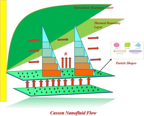
Figure 2 illustrates the inside geometry of the PTSC.

Figure 2. Solar collector in a schematic view.

2.4 Model equations

Impending the boundary layer, the prevailing equations corresponding to the Casson nanofluid flow and those related to heat transfer are derived in [49] (3) $\begin{array}{rl}\frac{\mathrm{\partial }{H}_1}{\mathrm{\partial }x}& +\frac{\mathrm{\partial }{H}_2}{\mathrm{\partial }y}=0,\end{array}$(3) (4) $\begin{array}{rl}{H}_1\frac{\mathrm{\partial }{H}_1}{\mathrm{\partial }x}+H_2\frac{\mathrm{\partial }{H}_1}{\mathrm{\partial }y}& =\frac{{\mu }_{nf}\left(B\right)}{{\rho }_{nf}}\left(1+\frac{1}{{\text{β}}_w}\right)\frac{{\mathrm{\partial }}^2{H}_1}{\mathrm{\partial }{y}^2}\\ & -\frac{{\sigma }_{nf}{B}^2{H}_1}{{\rho }_{nf}}-\frac{{\mu }_{nf}}{{\rho }_{nf}k}{H}_1,\end{array}$(4) (5) $\begin{array}{rl}{H}_1\frac{\mathrm{\partial }\mathrm{\Omega }}{\mathrm{\partial }x}+H_2\frac{\mathrm{\partial }\mathrm{\Omega }}{\mathrm{\partial }y}& =\frac{1}{{\left(\rho C_p\right)}_{nf}}\left[\frac{\mathrm{\partial }}{\mathrm{\partial }y}\left({\kappa }_{nf}^{\ast }\left(\mathrm{\Omega }\right)\frac{\mathrm{\partial }\mathrm{\Omega }}{\mathrm{\partial }y}\right)\right]\\ & +\frac{{\sigma }_{nf}}{{\left(\rho C_p\right)}_{nf}}{B}^2{H_1}^2-\frac{1}{{\left(\rho C_p\right)}_{nf}}\frac{\mathrm{\partial }{q}_r}{\mathrm{\partial }y}.\end{array}$(5)

2.5. Boundary conditions

The subsequent equations signify the boundary situations linked to the present model (for instance, see Jamshed [50]): (6) $\begin{array}{rl}{H}_1\left(x,0\right)& =U_w+N_L\left(1+\frac{1}{{\text{β}}_w}\right)\left(\frac{\mathrm{\partial }{H}_1}{\mathrm{\partial }y}\right),\\ H_2\left(x,0\right)& =V_{\mathrm{\Pi }},-k_{\mathrm{\Pi }}\left(\frac{\mathrm{\partial }\mathrm{\Omega }}{\mathrm{\partial }y}\right)=h_{\mathrm{\Pi }}\left({\mathrm{\Omega }}_w-\mathrm{\Omega }\right),\end{array}$(6) (7) $\begin{array}{rl}{H}_1& \to 0,\mathrm{\Omega }\to {\mathrm{\Omega }}_{\mathrm{\infty }}asy\to \mathrm{\infty }.\end{array}$(7) Here $H_1$ and $H_2$ signify velocities in the corresponding directions of $x$ and $y$, $N_L$ represents the slip length, while ${\rho }_{nf}$, ${\sigma }_{nf}$, and ${\kappa }_{nf}^{\ast }\left(\mathrm{\Omega }\right)$ respectively symbolize the density, electricalonductivity, and variable thermal conductivity associated with nanofluid. $q_r$ is a descriptive of the radiative heat flux while $(C_p{)}_{nf}$ stands for the specific heat capacity possessed by the nanofluid. $V_{\mathrm{\Pi }}$ symbolizes how porous the stretching surface is. $k_{\mathrm{\Pi }}$ is the solid thermal conductivity and $h_{\mathrm{\Pi }}$. represents the convective thermal transmitting factor.

2.6. Thermophysical properties corresponding to Casson nanofluid

In the base engine oil, the nanoparticles were suspended which causes enriched thermophysical properties. The subsequent equations encapsulate the material constraints for the Casson nanofluid [51–53]. (8) $\begin{array}{rl}\left.\begin{array}{c}{\mu }_{nf}={\mu }_f{(1-\varphi )}^{-2.5},\\ {\kappa }_{nf}^{\ast }\left(\mathrm{\Omega }\right)=k_{nf}\left[1+{ϵ}_w\frac{\mathrm{\Omega }-{\mathrm{\Omega }}_{\mathrm{\infty }}}{{\mathrm{\Omega }}_w-{\mathrm{\Omega }}_{\mathrm{\infty }}}\right],\\ {\left(\rho C_p\right)}_{nf}=\left(1-\varphi \right){\left(\rho C_p\right)}_f+\varphi {\left(\rho C_p\right)}_s,\\ \frac{{\rho }_{nf}}{{\rho }_f}=\left(1-\varphi \right)+\varphi \frac{{\rho }_s}{{\rho }_f},\end{array}\right\}& \end{array}$(8) (9) $\begin{array}{rl}\left.\begin{array}{c}\frac{{\sigma }_{nf}}{{\sigma }_f}=\left[1+\frac{3\left({\displaystyle \frac{{\sigma }_s}{{\sigma }_f}}-1\right)\varphi }{\left({\displaystyle \frac{{\sigma }_s}{{\sigma }_f}}+2\right)-\left({\displaystyle \frac{{\sigma }_s}{{\sigma }_f}}-1\right)\varphi }\right],\\ \frac{{\kappa }_{nf}}{{\kappa }_f}=\left[\frac{\left({\kappa }_s+\left(m-1\right){\kappa }_f\right)-\left(m-1\right)\varphi \left({\kappa }_f-{\kappa }_s\right)}{\left({\kappa }_s+\left(m-1\right){\kappa }_f\right)+\varphi \left({\kappa }_f-{\kappa }_s\right)}\right].\end{array}\right\}& \end{array}$(9) Here $\varphi$ is the fractional volume factor of nanoparticles. ${\kappa }_f$, ${\sigma }_f$, ${\mu }_f$, $(C_p{)}_f$, and ${\rho }_f$ are respectively the thermal and electrical conductivity, dynamic viscosity, active heat capacity, and also the density of the base level fluid. However, the same representation with subscript (s) represents the nanoparticle thermophysical characteristics.

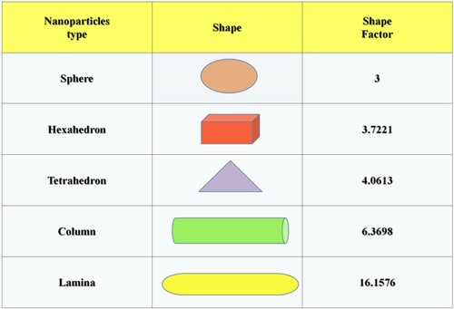
2.7. Nanoparticle shape aspect $\mathit{m}$

The scale of altered nanoparticle forms is acknowledged as the nanoparticle shape aspect. Figure 3 exemplifies the observed shape aspect values obtained for a variety of particle shapes [54].

Figure 3. Shape factor value for different particles shapes.

2.8. Nanoparticles and base fluid properties

The substantial properties of nanofluid with particle and engine oil with two dissimilar nanoparticles that are used in this research are specified in Table 1 [55–59].

Table 1. Substantial properties associated with nanoparticles and base fluid at 293 K.

Thermophysical	$\rho \left(\text{kg}/{\text{m}}^3\right)$	$c_p\left(\text{J}/\text{kgK}\right)$	$k\left(\text{W}/\text{mK}\right)$	$\sigma \left(\text{S}/\text{m}\right)$
Copper (Cu)	8933	385.0	401.00	5.96×10^7
Engine Oil (EO)	884	1910	0.144	0.125×10^−11
Iron (II, III) oxide (Fe3O4)	5180	670	9.7	0.112×10^6

2.9 Roseland approximations

Considering a non-Newtonian Casson nanofluid, only a short distance is travelled by radiation inside the fluid because of its thickness. Owing to this phenomenon, Rosseland approximation for radiative transfer [60] is used in Equation (5) and it is obtained that (10) $\begin{array}{r}{q}_r=-\frac{4{\sigma }^{\ast }}{3k^{\ast }}\frac{\mathrm{\partial }{\mathrm{\Omega }}^4}{\mathrm{\partial }y},\end{array}$(10) In which, ${\sigma }^{\ast }$ is used to represent the Stefan Boltzmann constant (a.k.a. Stefan constant) and $k^{\ast }$ known as absorption coefficient denotes the rate at which there is a decrease in incident radiation when depth increases.

3. Solving the problem

The PDEs system that directs the problem (3)–(7) is resolved by introducing stream functions $\psi$ as below (11) $\begin{array}{r}{H}_1=\frac{\mathrm{\partial }\psi }{\mathrm{\partial }y},H_2=-\frac{\mathrm{\partial }\psi }{\mathrm{\partial }x},\end{array}$(11) $\psi \left(x,y\right)$ signifies the stream function and the subsequent equations define the similarity variables: defined as (12) $\begin{array}{rl}{\ddot{\theta }}^{\ast }\left(x,y\right)& =\sqrt{\frac{n}{{\nu }_f}}y,\psi \left(x,y\right)=\sqrt{{\nu }_{f}n}xf\left({\ddot{\theta }}^{\ast }\right),\\ \theta \left({\ddot{\theta }}^{\ast }\right)& =\frac{\mathrm{\Omega }-{\mathrm{\Omega }}_{\mathrm{\infty }}}{{\mathrm{\Omega }}_w-{\mathrm{\Omega }}_{\mathrm{\infty }}}.\end{array}$(12)

Similarity transformation that is defined in Equations (11) and (12) is then used in Equations (3)–(7). Hence, non-dimensional equations are derived as follows. (13) $\begin{array}{rl}& \frac{1}{{\varphi }_1{\varphi }_2}\left(1+\frac{1}{{\text{β}}_w}\right)f^{\mathrm{\prime }\mathrm{\prime }\mathrm{\prime }}+f{f}^{\mathrm{\prime }\mathrm{\prime }}-f^{{\mathrm{\prime }}^2}\\ & -\frac{{\varphi }_4}{{\varphi }_2}{M}_w{f}^{\mathrm{\prime }}-\frac{1}{{\varphi }_1}{K}_w{f}^{\mathrm{\prime }}=0,\end{array}$(13) (14) $\begin{array}{rl}& {\theta }^{\mathrm{\prime }\mathrm{\prime }}\left(1+{ϵ}_w\theta +\frac{1}{{\varphi }_5}{P}_r{N}_w\right)+{ϵ}_w{\theta }^{{\mathrm{\prime }}^2}\\ & +P_r\frac{{\varphi }_3}{{\varphi }_5}\left[f{\theta }^{\mathrm{\prime }}-f^{\mathrm{\prime }}\theta +\frac{{\varphi }_4}{{\varphi }_3}{M}_w{E}_w{f}^{{\mathrm{\prime }}^2}\right]=0,\end{array}$(14) (15) $\begin{array}{rl}f\left(0\right)& =S,f^{\mathrm{\prime }}\left(0\right)=1+{\mathrm{\Lambda }}_w\left(1+\frac{1}{{\text{β}}_w}\right)f^{\mathrm{\prime }\mathrm{\prime }}\left(0\right),\\ {\theta }^{\mathrm{\prime }}\left(0\right)& =-B_w\left(1-\theta \left(0\right)\right),\end{array}$(15) (16) $\begin{array}{rl}{f}^{\mathrm{\prime }}\left({\ddot{\theta }}^{\ast }\right)& \to 0,\theta \left({\ddot{\theta }}^{\ast }\right)\to 0,\text{ as}{\ddot{\theta }}^{\ast }\to \mathrm{\infty },\end{array}$(16) where (17) $\begin{array}{rl}{\varphi }_1& =(1-\varphi {)}^{2.5},{\varphi }_2=\left(1-\varphi +\varphi \frac{{\rho }_s}{{\rho }_f}\right),\\ {\varphi }_3& =\left(1-\varphi +\varphi \frac{{\left(\rho C_p\right)}_s}{{\left(\rho C_p\right)}_f}\right),\end{array}$(17) (18) $\begin{array}{rl}{\varphi }_4& =\left(1+\frac{3\left(\frac{{\sigma }_s}{{\sigma }_f}-1\right)\varphi }{\left(\frac{{\sigma }_s}{{\sigma }_f}+2\right)-\left(\frac{{\sigma }_s}{{\sigma }_f}-1\right)\varphi }\right),\\ {\varphi }_5& =\left(\frac{\left(k_s+\left(m-1\right)k_f\right)-\left(m-1\right)\varphi \left(k_f-k_s\right)}{\left(k_s+\left(m-1\right)k_f\right)+\varphi \left(k_f-k_s\right)}\right).\end{array}$(18) In the equations above, the differentiation according to ${\ddot{\theta }}^{\ast }$ is represented by prime, the porous media and magnetic parameters are represented by $K_w={\nu }_f/nk$, $M_w={\sigma }_f{B}^2/c{\rho }_f$, respectively. $P_r={\nu }_f/{\alpha }_f$ denotes the Prandtl number, ${\alpha }_f={\kappa }_f/{\left(\rho C_p\right)}_f$ and $N_w=16/3{\sigma }^{\ast }{\mathrm{\Omega }}_{\mathrm{\infty }}^3/{\kappa }^{\ast }{\nu }_f{\left(\rho C_p\right)}_f$ are the heat diffusivity and radiation constraints, respectively. $E_w=U_w^2/{\left(C_p\right)}_f\left(T_w-T_{\mathrm{\infty }}\right)$ represents the Eckert number. $S=-V_w\sqrt{\frac{1}{{\nu }_{f}c}}$ stands for the mass transfer parameter, ${\mathrm{\Lambda }}_w=\sqrt{\frac{n}{{\nu }_f}}{N}_L$ denotes the velocity slip parameter, and $B_w=\frac{h_f}{k_f}\sqrt{\frac{{\nu }_f}{n}}$ represents the Biot number.

4. Numerical practice: Keller box method

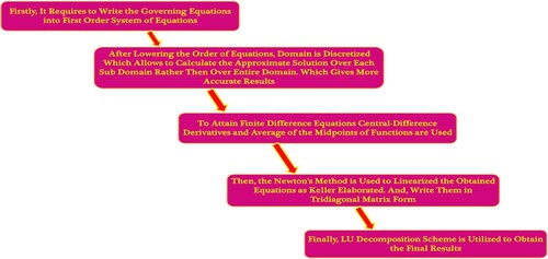
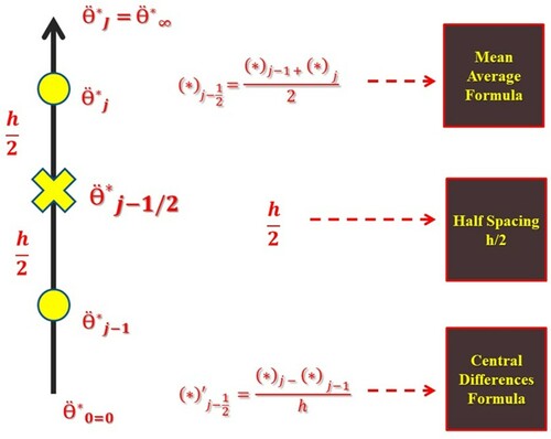
It is complex to analytically solve a set of nonlinear systems of ODEs (13) and (14), arising as an output of mathematical modelling for the given physical system that corresponds to nanofluid flow. Thus, to find the numerical approximate solutions, a Keller box technique [61] scheme is employed. Being also recognized as the inherent finite difference method, this scheme is intrinsically steady, and to elaborate more, it is second-order convergent. The following flow chart explains the procedure of the Keller box method (Figure 4).

Figure 4. Flow chart of Keller box method.

4.1 Step 1: transfiguration of ODEs

There are several steps involved in the completion of the method. The first step involves the conversion of the ODEs (13)–(16) into a completed first-order system of codes. (19) $\begin{array}{rl}& D_1=f^{\mathrm{\prime }},\end{array}$(19) (20) $\begin{array}{rl}& D_2={H_1}^{{}^{\mathrm{\prime }}},\end{array}$(20) (21) $\begin{array}{rl}& D_3={\theta }^{\mathrm{\prime }},\end{array}$(21) (22) $\begin{array}{rl}& \frac{1}{{\varphi }_1{\varphi }_2}\left(1+\frac{1}{{\text{β}}_w}\right)D_2^{{}^{\mathrm{\prime }}}+f{D}_2-D_1^2-\frac{{\varphi }_4}{{\varphi }_2}{M}_w{D}_1\\ & -\frac{1}{{\varphi }_1}{K}_w{D}_1=0,\end{array}$(22) (23) $\begin{array}{rl}& D_3^{{}^{\mathrm{\prime }}}\left(1+{ϵ}_w\theta +\frac{1}{{\varphi }_5}{P}_r{N}_w\right)+{ϵ}_w{D}_3^2\\ & +P_r\frac{{\varphi }_3}{{\varphi }_5}\left[f{D}_3-D_1\theta +\frac{{\varphi }_4}{{\varphi }_3}{M}_w{E}_w{D}_1^2\right]=0.\end{array}$(23) (24) $\begin{array}{rl}f\left(0\right)& =S,D_1\left(0\right)=1+{\mathrm{\Lambda }}_w\left(1+\frac{1}{{\text{β}}_w}\right)D_2\left(0\right),\\ D_3\left(0\right)& =-B_w\left(1-\theta \left(0\right)\right),D_1\left(\mathrm{\infty }\right)\to 0,\theta \left(\mathrm{\infty }\right)\to 0.\end{array}$(24)

4.2 Step 2: discretization of domain

Once the first-order system is obtained, domain discretization must be conducted to determine the approximate solution. To do so, the domain is usually divided into a uniform grid. Highly accurate numerical results can be achieved by a relatively smaller grid (Figure 5). ${{\ddot{\theta }}^{\ast }}_0=0,{{\ddot{\theta }}^{\ast }}_j={{\ddot{\theta }}^{\ast }}_{j-1}+h,j=1,2,3,\dots ,J-1,{{\ddot{\theta }}^{\ast }}_J={{\ddot{\theta }}^{\ast }}_{\mathrm{\infty }}.$In this case, $h=0.01$ is fixed. Afterward, difference equations are derived utilizing central differences. A replacement of functions with their associated mean averages is also conducted. Next, the ordinary differential system (19)–(24) is reduced to the nonlinear algebraic equations as follows. (25) $\begin{array}{rl}& \frac{{\left(D_1\right)}_j+{\left(D_1\right)}_{j-1}}{2}=\frac{f_j-f_{j-1}}{h},\end{array}$(25) (26) $\begin{array}{rl}& \frac{{\left(D\right)}_j+{\left(D_2\right)}_{j-1}}{2}=\frac{{\left(D_1\right)}_j-{\left(D_1\right)}_{j-1}}{h},\end{array}$(26) (27) $\begin{array}{rl}& \frac{{\left(D_3\right)}_j+{\left(D_3\right)}_{j-1}}{2}=\frac{{\theta }_j-{\theta }_{j-1}}{h},\end{array}$(27) (28) $\begin{array}{rl}& \frac{1}{{\varphi }_1{\varphi }_2}\left(1+\frac{1}{{\text{β}}_w}\right)\left(\frac{{\left(D_2\right)}_j-{\left(D_2\right)}_{j-1}}{h}\right)\\ & +\left(\frac{f_j+f_{j-1}}{2}\right)\left(\frac{{\left(D_2\right)}_j+{\left(z_2\right)}_{j-1}}{2}\right)\\ & -{\left(\frac{{\left(D_1\right)}_j+{\left(D_1\right)}_{j-1}}{2}\right)}^2\\ & -\frac{{\varphi }_4}{{\varphi }_3}{M}_w\left(\frac{{\left(D_1\right)}_j+{\left(D_2\right)}_{j-1}}{2}\right)\\ & -K_w\frac{1}{{\varphi }_1}\left(\frac{{\left(D_1\right)}_j+{\left(D_1\right)}_{j-1}}{2}\right)=0\end{array}$(28) (29) $\begin{array}{rl}& \left(\frac{{\left(D_3\right)}_j-{\left(D_3\right)}_{j-1}}{h}\right)\left(1+{ϵ}_w\left(\frac{{\theta }_j+{\theta }_{j-1}}{2}\right)+\frac{1}{{\varphi }_5}{P}_r{N}_w\right)\\ & +{ϵ}_w{\left(\frac{{\left(D_3\right)}_j+{\left(D_3\right)}_{j-1}}{2}\right)}^2\\ & +P_r\frac{{\varphi }_3}{{\varphi }_5}\left[\left(\frac{f_j+f_{j-1}}{2}\right)\left(\frac{{\left(D_3\right)}_j+{\left(D_3\right)}_{j-1}}{2}\right)\right]\\ & +P_r\frac{{\varphi }_3}{{\varphi }_5}\left[\left(\frac{{\left(z_1\right)}_j+{\left(z_1\right)}_{j-1}}{2}\right)\left(\frac{{\theta }_j+{\theta }_{j-1}}{2}\right)\right.\\ & -\left.\frac{{\varphi }_4}{{\varphi }_3}{M}_w{E}_w{\left(\frac{{\left(D_1\right)}_j+{\left(D_1\right)}_{j-1}}{2}\right)}^2\right]=0\end{array}$(29)

Figure 5. Net rectangle for difference approximations

4.3 Step 3: linearized utilizing Newton's method

Now, Newton's method is utilized to linearize the ensuing algebraic equations, i.e: (30) $\begin{array}{r}({)}_j^{\left(i+1\right)}=({)}_j^{\left(i\right)}+\mathrm{{\rm Y}}({)}_j^{\left(i\right)},\end{array}$(30) Hence, by substituting this into Equations (25)–(29) along with ignoring ${\mathrm{{\rm Y}}}_j^i$ in higher terms, the below system is determined as a linear tridiagonal system. (31) $\begin{array}{rl}& \mathrm{{\rm Y}}{f}_j-\mathrm{{\rm Y}}{f}_{j-1}-\frac{1}{2}h\left(\mathrm{{\rm Y}}{D_1}_j+\mathrm{{\rm Y}}{D_1}_{j-1}\right)=(r_1{)}_{j-\frac{1}{2}},\end{array}$(31) (32) $\begin{array}{rl}& \mathrm{{\rm Y}}{D_1}_j-\mathrm{{\rm Y}}{D_1}_{j-1}-\frac{1}{2}h\left(\mathrm{{\rm Y}}{D_2}_j+\mathrm{{\rm Y}}{D_2}_{j-1}\right)=(r_2{)}_{j-\frac{1}{2}},\end{array}$(32) (33) $\begin{array}{rl}& \mathrm{{\rm Y}}{\theta }_j-\mathrm{{\rm Y}}{\theta }_{j-1}-\frac{1}{2}h(\mathrm{{\rm Y}}(D_3{)}_j+\mathrm{{\rm Y}}(D_3{)}_{j-1})=(r_3{)}_{j-\frac{1}{2}},\end{array}$(33) (34) $\begin{array}{rl}& {\left(a_1\right)}_j\mathrm{{\rm Y}}{f}_j+{\left(a_2\right)}_j\mathrm{{\rm Y}}{f}_{j-1}+{\left(a_3\right)}_j\mathrm{{\rm Y}}{D_1}_j+{\left(a_4\right)}_j\mathrm{{\rm Y}}{D_1}_{j-1}\\ & +{\left(a_5\right)}_j\mathrm{{\rm Y}}{D_2}_j+{\left(a_6\right)}_j\mathrm{{\rm Y}}{D_2}_{j-1}\\ & +{\left(a_7\right)}_j\mathrm{{\rm Y}}{\theta }_j+{\left(a_8\right)}_j\mathrm{{\rm Y}}{\theta }_{j-1}+{\left(a_9\right)}_j\mathrm{{\rm Y}}{\left(D_3\right)}_j\\ & +{\left(a_{10}\right)}_j\mathrm{{\rm Y}}{\left(D_3\right)}_{j-1}={\left(r_4\right)}_{j-\frac{1}{2}},\end{array}$(34) (35) $\begin{array}{rl}& {\left(b_1\right)}_j\mathrm{{\rm Y}}{f}_j+{\left(b_2\right)}_j\mathrm{{\rm Y}}{f}_{j-1}+{\left(b_3\right)}_j\mathrm{{\rm Y}}{D_1}_j+{\left(b_4\right)}_j\mathrm{{\rm Y}}{D_1}_{j-1}\\ & +{\left(b_5\right)}_j\mathrm{{\rm Y}}{D_2}_j+{\left(b_6\right)}_j\mathrm{{\rm Y}}{D_2}_{j-1}\\ & +{\left(b_7\right)}_j\mathrm{{\rm Y}}{\theta }_j+{\left(b_8\right)}_j\mathrm{{\rm Y}}{\theta }_{j-1}+{\left(b_9\right)}_j\mathrm{{\rm Y}}{\left(D_3\right)}_j\\ & +{\left(b_{10}\right)}_j\mathrm{{\rm Y}}{\left(D_3\right)}_{j-1}={\left(r_5\right)}_{j-\frac{1}{2}}.\end{array}$(35) where (36) $\begin{array}{rl}(r_1{)}_{j-\frac{1}{2}}& =-f_j+f_{j-1}+\frac{h}{2}\left({D_1}_j+{D_1}_{j-1}\right),\end{array}$(36) (37) $\begin{array}{rl}(r_2{)}_{j-\frac{1}{2}}& =-{D_1}_j+{D_1}_{j-1}+\frac{h}{2}\left({D_2}_j+{D_2}_{j-1}\right),\end{array}$(37) (38) $\begin{array}{rl}(r_3{)}_{j-\frac{1}{2}}& =-{\theta }_j+{\theta }_{j-1}+\frac{h}{2}((D_3{)}_j+(D_3{)}_{j-1}),\end{array}$(38) (39) $\begin{array}{rl}(r_4{)}_{j-\frac{1}{2}}& =-h\left[\left(1+\frac{1}{{\text{β}}_w}\right)\left(\frac{({\left(D_2\right)}_j-(D_2{)}_{j-1})}{{\varphi }_1{\varphi }_{2}h}\right)\right.\\ & +\left(\frac{\left(f_j+f_{j-1}\right)({\left(D_2\right)}_j+(D_2{)}_{j-1})}{4}\right)\\ & -\left.\left(\frac{{\left({\left(D_1\right)}_j+{\left(D_1\right)}_{j-1}\right)}^2}{4}\right)\right]\\ & +h\left[\frac{{\varphi }_4}{{\varphi }_2}{M}_w\left(\frac{\left({\left(D_1\right)}_j+{\left(D_1\right)}_{j-1}\right)}{2}\right)\right.\\ & +\left.K_w\frac{1}{{\varphi }_1}\left(\frac{{\left(D_1\right)}_j+{\left(D_1\right)}_{j-1}}{2}\right)\right],\end{array}$(39) (40) $\begin{array}{rl}(r_5{)}_{j-\frac{1}{2}}& =-h[\frac{\begin{array}{c}\left({\left(D_3\right)}_j-{\left(D_3\right)}_{j-1}\right)\\ \left(1+{ϵ}_w\left(\frac{{\theta }_j+{\theta }_{j-1}}{2}\right)+\frac{1}{{\varphi }_5}{P}_r{N}_r\right)\end{array}}{h}]\\ & -h\left[{ϵ}_w{\left(\frac{{\left(D_3\right)}_j+{\left(D_3\right)}_{j-1}}{2}\right)}^2\right]\\ & -h\frac{{\varphi }_3}{{\varphi }_5}{P}_r\left[\left(\frac{\left({\theta }_j+{\theta }_{j-1}\right)({\left(D_1\right)}_j+(D_1{)}_{j-1})}{4}\right)\right.\\ & -\left.\frac{{\varphi }_4}{{\varphi }_3}{M}_w{E}_w{\left(\frac{{\left(D_1\right)}_j+{\left(D_1\right)}_{j-1}}{2}\right)}^2\right].\end{array}$(40)

Using the similarity process the boundary conditions become (41) $\begin{array}{rl}\mathrm{{\rm Y}}{f}_0& =0,\mathrm{{\rm Y}}(D_1{)}_0=0,\mathrm{{\rm Y}}(D_3{)}_0=0,\mathrm{{\rm Y}}(D_1{)}_J=0,\\ \mathrm{{\rm Y}}{\theta }_J& =0,\end{array}$(41)

4.4 The Block tridiagonal matrix

The linearized differential Equations (30)–(35) have a block tridiagonal structure.

The system is written in a matrix-vector form as follows,

For $j=1;$ (42) $\begin{array}{rl}& \mathrm{{\rm Y}}{f}_1-\mathrm{{\rm Y}}{f}_0-\frac{1}{2}h(\mathrm{{\rm Y}}(D_1{)}_1+\mathrm{{\rm Y}}(D_1{)}_0)=(r_1{)}_{1-\frac{1}{2}},\end{array}$(42) (43) $\begin{array}{rl}& \mathrm{{\rm Y}}(D_1{)}_1-\mathrm{{\rm Y}}(D_1{)}_0-\frac{1}{2}h(\mathrm{{\rm Y}}(D_2{)}_1+\mathrm{{\rm Y}}(D_2{)}_0)\\ & =(r_2{)}_{1-\frac{1}{2}},\end{array}$(43) (44) $\begin{array}{rl}& \mathrm{{\rm Y}}{\theta }_1-\mathrm{{\rm Y}}{\theta }_0-\frac{1}{2}h(\mathrm{{\rm Y}}(D_3{)}_1+\mathrm{{\rm Y}}(D_3{)}_0)=(r_3{)}_{1-\frac{1}{2}},\end{array}$(44) (45) $\begin{array}{rl}& {\left(a_1\right)}_1\mathrm{{\rm Y}}{f}_1+{\left(a_2\right)}_1\mathrm{{\rm Y}}{f}_0+{\left(a_3\right)}_1\mathrm{{\rm Y}}{\left(D_1\right)}_1+{\left(a_4\right)}_1\mathrm{{\rm Y}}{\left(D_1\right)}_0\\ & +{\left(a_5\right)}_1\mathrm{{\rm Y}}{\left(D_2\right)}_1+{\left(a_6\right)}_1\mathrm{{\rm Y}}{\left(D_2\right)}_0+{\left(a_7\right)}_1\mathrm{{\rm Y}}{\theta }_j\\ & +{\left(a_8\right)}_1\mathrm{{\rm Y}}{\theta }_0+{\left(a_9\right)}_1\mathrm{{\rm Y}}{\left(\text{D}\right)}_1+{\left(a_{10}\right)}_1\mathrm{{\rm Y}}{\left(D_3\right)}_0\\ & ={\left(r_4\right)}_{1-\frac{1}{2}},\end{array}$(45) (46) $\begin{array}{rl}& {\left(b_1\right)}_1\mathrm{{\rm Y}}{f}_1+{\left(b_2\right)}_1\mathrm{{\rm Y}}{f}_0+{\left(b_3\right)}_1\mathrm{{\rm Y}}{\left(D_1\right)}_1+{\left(b_4\right)}_1\mathrm{{\rm Y}}{\left(D_1\right)}_0\\ & +{\left(b_5\right)}_1\mathrm{{\rm Y}}{\left(D_2\right)}_1+{\left(b_6\right)}_1\mathrm{{\rm Y}}{\left(z_2\right)}_0+{\left(b_7\right)}_1\mathrm{{\rm Y}}{\theta }_1\\ & +{\left(b_8\right)}_1\mathrm{{\rm Y}}{\theta }_0+{\left(b_9\right)}_1\mathrm{{\rm Y}}{\left(D_3\right)}_1+{\left(b_{10}\right)}_1\mathrm{{\rm Y}}{\left(D_3\right)}_0\\ & ={\left(r_5\right)}_{1-\frac{1}{2}}.\end{array}$(46)

In matrix form, (47) $\begin{array}{rl}& \left[\begin{array}{ccccc}0& 0& 1& 0& 0\\ -h/2& 0& 0& -h/2& 0\\ 0& -h/2& 0& 0& -h/2\\ {\left(a_2\right)}_1& {\left(a_{10}\right)}_1& {\left(a_3\right)}_1& {\left(a_1\right)}_1& {\left(a_9\right)}_1\\ {\left(b_2\right)}_1& {\left(b_{10}\right)}_1& {\left(b_3\right)}_1& {\left(b_1\right)}_1& {\left(b_9\right)}_1\end{array}\right]\left[\begin{array}{l}\mathrm{{\rm Y}}{\left(D_2\right)}_0\\ \mathrm{{\rm Y}}{\left(\theta \right)}_0\\ \mathrm{{\rm Y}}{\left(f\right)}_1\\ \mathrm{{\rm Y}}{\left(D_2\right)}_1\\ \mathrm{{\rm Y}}{\left(D_3\right)}_1\end{array}\right]\\ & +\left[\begin{array}{ccccc}-h/2& 0& 0& 0& 0\\ 1& 0& 0& 0& 0\\ 0& 1& 0& 0& 0\\ {\left(a_5\right)}_1& {\left(a_7\right)}_1& 0& 0& 0\\ {\left(b_5\right)}_1& {\left(b_7\right)}_1& 0& 0& 0\end{array}\right]\left[\begin{array}{l}\mathrm{{\rm Y}}{\left(D_1\right)}_1\\ \mathrm{{\rm Y}}{\left(\theta \right)}_1\\ \mathrm{{\rm Y}}{\left(f\right)}_2\\ \mathrm{{\rm Y}}{\left(D_2\right)}_2\\ \mathrm{{\rm Y}}{\left(D_3\right)}_2\end{array}\right]\\ & =\left[\begin{array}{l}{\left(r_1\right)}_{\frac{1}{2}}\\ {\left(r_2\right)}_{\frac{1}{2}}\\ {\left(r_3\right)}_{\frac{1}{2}}\\ {\left(r_4\right)}_{\frac{1}{2}}\\ {\left(r_5\right)}_{\frac{1}{2}}\end{array}\right]\end{array}$(47)

That is (48) $\begin{array}{r}\left[A_1\right]\left[{\mathrm{{\rm Y}}}_1\right]+\left[C_1\right]\left[{\mathrm{{\rm Y}}}_2\right]=\left[r_1\right].\end{array}$(48)

For $j=2;$ (49) $\begin{array}{rl}& \mathrm{{\rm Y}}{f}_2-\mathrm{{\rm Y}}{f}_1-\frac{1}{2}h(\mathrm{{\rm Y}}(D_1{)}_2+\mathrm{{\rm Y}}(D_1{)}_1)=(r_1{)}_{1-\frac{1}{2}},\end{array}$(49) (50) $\begin{array}{rl}& \mathrm{{\rm Y}}(D_1{)}_2-\mathrm{{\rm Y}}(D_1{)}_1-\frac{1}{2}h(\mathrm{{\rm Y}}(D_2{)}_2+\mathrm{{\rm Y}}(D_2{)}_1)\\ & =(r_2{)}_{1-\frac{1}{2}},\end{array}$(50) (51) $\begin{array}{rl}& \mathrm{{\rm Y}}{\theta }_1-\mathrm{{\rm Y}}{\theta }_0-\frac{1}{2}h(\mathrm{{\rm Y}}(D_3{)}_2+\mathrm{{\rm Y}}(D_3{)}_1)=(r_3{)}_{1-\frac{1}{2}},\end{array}$(51) (52) $\begin{array}{rl}& {\left(a_1\right)}_2\mathrm{{\rm Y}}{f}_2+{\left(a_2\right)}_2\mathrm{{\rm Y}}{f}_1+{\left(a_3\right)}_2\mathrm{{\rm Y}}{\left(D_1\right)}_2+{\left(a_4\right)}_2\mathrm{{\rm Y}}{\left(D_1\right)}_1\\ & +{\left(a_5\right)}_2\mathrm{{\rm Y}}{\left(D_2\right)}_2+{\left(a_6\right)}_2\mathrm{{\rm Y}}{\left(D_2\right)}_1+{\left(a_7\right)}_2\mathrm{{\rm Y}}{\theta }_2\\ & +{\left(a_8\right)}_2\mathrm{{\rm Y}}{\theta }_1+{\left(a_9\right)}_2\mathrm{{\rm Y}}{\left(D_3\right)}_2+{\left(a_{10}\right)}_2\mathrm{{\rm Y}}{\left(D_3\right)}_1\\ & ={\left(r_4\right)}_{2-\frac{1}{2}},\end{array}$(52) (53) $\begin{array}{rl}& {\left(b_1\right)}_2\mathrm{{\rm Y}}{f}_2+{\left(b_2\right)}_2\mathrm{{\rm Y}}{f}_1+{\left(b_3\right)}_2\mathrm{{\rm Y}}{\left(D_1\right)}_2+{\left(b_4\right)}_2\mathrm{{\rm Y}}{\left(D_1\right)}_1\\ & +{\left(b_5\right)}_2\mathrm{{\rm Y}}{\left(D_2\right)}_2+{\left(b_6\right)}_2\mathrm{{\rm Y}}{\left(D_2\right)}_1+{\left(b_7\right)}_2\mathrm{{\rm Y}}{\theta }_2\\ & +{\left(b_8\right)}_2\mathrm{{\rm Y}}{\theta }_1+{\left(b_9\right)}_2\mathrm{{\rm Y}}{\left(D_3\right)}_2+{\left(b_{10}\right)}_2\mathrm{{\rm Y}}{\left(D_3\right)}_1\\ & ={\left(r_5\right)}_{2-\frac{1}{2}}.\end{array}$(53)

In matrix form, (54) $\begin{array}{rl}& \left[\begin{array}{ccccc}0& 0& -1& 0& 0\\ 0& 0& 0& -h/2& 0\\ 0& 0& 0& 0& -h/2\\ 0& 0& {\left(a_4\right)}_2& {\left(a_2\right)}_2& {\left(a_{10}\right)}_2\\ 0& 0& {\left(b_4\right)}_2& {\left(b_2\right)}_2& {\left(b_{10}\right)}_2\end{array}\right]\left[\begin{array}{l}\mathrm{{\rm Y}}{\left(D_2\right)}_0\\ \mathrm{{\rm Y}}{\left(\theta \right)}_0\\ \mathrm{{\rm Y}}{\left(f\right)}_1\\ \mathrm{{\rm Y}}{\left(D_2\right)}_1\\ \mathrm{{\rm Y}}{\left(D_3\right)}_1\end{array}\right]\\ & \times \left[\begin{array}{ccccc}-h/2& 0& 1& 0& 0\\ -1& 0& 0& -h/2& 0\\ 0& -1& 0& 0& -h/2\\ {\left(a_6\right)}_2& {\left(a_8\right)}_2& {\left(a_3\right)}_2& {\left(a_1\right)}_2& {\left(a_9\right)}_2\\ {\left(b_6\right)}_2& {\left(b_8\right)}_2& {\left(b_3\right)}_2& {\left(b_1\right)}_2& {\left(b_9\right)}_2\end{array}\right]\left[\begin{array}{l}\mathrm{{\rm Y}}{\left(D_1\right)}_1\\ \mathrm{{\rm Y}}{\left(\theta \right)}_1\\ \mathrm{{\rm Y}}{\left(f\right)}_2\\ \mathrm{{\rm Y}}{\left(D_2\right)}_2\\ \mathrm{{\rm Y}}{\left(D_3\right)}_2\end{array}\right]\\ & +\left[\begin{array}{ccccc}-h/2& 0& 1& 0& 0\\ 1& 0& 0& -h/2& 0\\ 0& 1& 0& 0& -h/2\\ {\left(a_5\right)}_2& {\left(a_7\right)}_2& 0& 0& 0\\ {\left(b_5\right)}_2& {\left(b_7\right)}_2& 0& 0& 0\end{array}\right]\left[\begin{array}{l}\mathrm{{\rm Y}}{\left(D_1\right)}_1\\ \mathrm{{\rm Y}}{\left(\theta \right)}_1\\ \mathrm{{\rm Y}}{\left(f\right)}_2\\ \mathrm{{\rm Y}}{\left(D_2\right)}_2\\ \mathrm{{\rm Y}}{\left(D_3\right)}_2\end{array}\right]\\ & =\left[\begin{array}{l}{\left(r_1\right)}_{\frac{3}{2}}\\ {\left(r_2\right)}_{\frac{3}{2}}\\ {\left(r_3\right)}_{\frac{3}{2}}\\ {\left(r_4\right)}_{\frac{3}{2}}\\ {\left(r_5\right)}_{\frac{3}{2}}\end{array}\right].\end{array}$(54) That is (55) $\begin{array}{r}\left[B_2\right]\left[{\mathrm{{\rm Y}}}_1\right]+\left[A_2\right]\left[{\mathrm{{\rm Y}}}_2\right]+\left[C_2\right]\left[{\mathrm{{\rm Y}}}_3\right]=\left[r_2\right].\end{array}$(55)

For $j=J-1;$ (56) $\begin{array}{rl}& \mathrm{{\rm Y}}{f}_{J-1}-\mathrm{{\rm Y}}{f}_{J-2}-\frac{1}{2}h\left(\mathrm{{\rm Y}}\right(\text{D}{)}_{J-1}+\mathrm{{\rm Y}}{D_1}_{J-2})\\ & =(r_1{)}_{J-1-\frac{1}{2}},\end{array}$(56) (57) $\begin{array}{rl}& \mathrm{{\rm Y}}(D_1{)}_{J-1}-\mathrm{{\rm Y}}(D_1{)}_{J-2}-\frac{1}{2}h(\mathrm{{\rm Y}}(D_2{)}_{J-1}+\mathrm{{\rm Y}}(D_2{)}_{J-2})\\ & =(r_2{)}_{J-1-\frac{1}{2}},\end{array}$(57) (58) $\begin{array}{rl}& \mathrm{{\rm Y}}{\theta }_{J-1}-\mathrm{{\rm Y}}{\theta }_{J-2}-\frac{1}{2}h(\mathrm{{\rm Y}}(D_3{)}_{J-1}+\mathrm{{\rm Y}}(D_3{)}_{J-2})\\ & =(r_3{)}_{J-1-\frac{1}{2}},\end{array}$(58) (59) $\begin{array}{rl}& {\left(a_1\right)}_{J-1}\mathrm{{\rm Y}}{f}_{J-1}+{\left(a_2\right)}_{J-1}\mathrm{{\rm Y}}{f}_{J-2}+{\left(a_3\right)}_{J-1}\mathrm{{\rm Y}}{\left(D_1\right)}_{J-1}\\ & +{\left(a_4\right)}_{J-1}\mathrm{{\rm Y}}{\left(D_1\right)}_{J-2}+{\left(a_5\right)}_{J-1}\mathrm{{\rm Y}}{\left(D_2\right)}_j\\ & +{\left(a_6\right)}_{J-1}\mathrm{{\rm Y}}{\left(D_2\right)}_{J-2}+{\left(a_7\right)}_{J-1}\mathrm{{\rm Y}}{\theta }_{J-1}\\ & +{\left(a_8\right)}_{J-1}\mathrm{{\rm Y}}{\theta }_{J-2}+{\left(a_9\right)}_{J-1}\mathrm{{\rm Y}}{\left(D_3\right)}_{J-1}\\ & +{\left(a_{10}\right)}_{J-1}\mathrm{{\rm Y}}{\left(D_3\right)}_{J-2}={\left(r_4\right)}_{J-1-\frac{1}{2}},\end{array}$(59) (60) $\begin{array}{rl}& {\left(b_1\right)}_{J-1}\mathrm{{\rm Y}}{f}_{J-1}+{\left(b_2\right)}_{J-1}\mathrm{{\rm Y}}{f}_{J-2}+{\left(b_3\right)}_{J-1}\mathrm{{\rm Y}}{\left(D_1\right)}_{J-1}\\ & +{\left(b_4\right)}_{J-1}\mathrm{{\rm Y}}{\left(z_1\right)}_{J-2}+{\left(b_5\right)}_{J-1}\mathrm{{\rm Y}}{\left(D_2\right)}_{J-1}\\ & +{\left(b_6\right)}_{J-1}\mathrm{{\rm Y}}{\left(D_2\right)}_{J-2}+{\left(b_7\right)}_{J-1}\mathrm{{\rm Y}}{\theta }_{J-1}\\ & +{\left(b_8\right)}_{J-1}\mathrm{{\rm Y}}{\theta }_{J-2}+{\left(b_9\right)}_{J-1}\mathrm{{\rm Y}}{\left(D_3\right)}_{J-1}\\ & +{\left(b_{10}\right)}_{J-1}\mathrm{{\rm Y}}{\left(D_3\right)}_{J-2}={\left(r_5\right)}_{J-1-\frac{1}{2}}.\end{array}$(60)

In matrix form, (61) $\begin{array}{rl}& \left[\begin{array}{ccccc}0& 0& -1& 0& 0\\ 0& 0& 0& -h/2& 0\\ 0& 0& 0& 0& -h/2\\ 0& 0& {\left(a_4\right)}_{J-2}& {\left(a_2\right)}_{J-2}& {\left(a_{10}\right)}_{J/2}\\ 0& 0& {\left(b_4\right)}_{J-2}& {\left(b_2\right)}_{J-2}& {\left(b_{10}\right)}_{J-2}\end{array}\right]\left[\begin{array}{l}\mathrm{{\rm Y}}{\left(D_2\right)}_{J-2}\\ \mathrm{{\rm Y}}{\left(\theta \right)}_{J-2}\\ \mathrm{{\rm Y}}{\left(f\right)}_{J-1}\\ \mathrm{{\rm Y}}{\left(D_2\right)}_{J-1}\\ \mathrm{{\rm Y}}{\left(D_3\right)}_{J-1}\end{array}\right]\\ & +\left[\begin{array}{ccccc}-h/2& 0& 0& 0& 0\\ 1& 0& 0& 0& 0\\ 0& 1& 0& 0& 0\\ {\left(a_5\right)}_{J-2}& {\left(a_9\right)}_{J-2}& 0& 0& 0\\ {\left(b_5\right)}_{J-2}& {\left(b_9\right)}_{J-2}& 0& 0& 0\end{array}\right]\left[\begin{array}{l}\mathrm{{\rm Y}}{\left(D_2\right)}_{J-2}\\ \mathrm{{\rm Y}}{\left(\theta \right)}_{J-2}\\ \mathrm{{\rm Y}}{\left(f\right)}_{J-1}\\ \mathrm{{\rm Y}}{\left(D_2\right)}_{J-1}\\ \mathrm{{\rm Y}}{\left(D_3\right)}_{J-1}\end{array}\right]\\ & +\left[\begin{array}{ccccc}-h/2& 0& 0& 0& 0\\ 1& 0& 0& 0& 0\\ 0& 1& 0& 0& 0\\ {\left(a_5\right)}_{J-2}& {\left(a_9\right)}_{J-2}& 0& 0& 0\\ {\left(b_5\right)}_{J-2}& {\left(b_9\right)}_{J-2}& 0& 0& 0\end{array}\right]\left[\begin{array}{l}\mathrm{{\rm Y}}{\left(D_1\right)}_{J-1}\\ \mathrm{{\rm Y}}{\left(\theta \right)}_{J-1}\\ \mathrm{{\rm Y}}{\left(f\right)}_J\\ \mathrm{{\rm Y}}{\left(D_2\right)}_J\\ \mathrm{{\rm Y}}{\left(D_3\right)}_J\end{array}\right]\\ & =\left[\begin{array}{l}{\left(r_1\right)}_{\left(J-1\right)-\frac{1}{2}}\\ {\left(r_2\right)}_{\left(J-1\right)-\frac{1}{2}}\\ {\left(r_3\right)}_{\left(J-1\right)-\frac{1}{2}}\\ {\left(r_4\right)}_{\left(J-1\right)-\frac{1}{2}}\\ {\left(r_5\right)}_{\left(J-1\right)-\frac{1}{2}}\end{array}\right].\end{array}$(61) That is (62) $\begin{array}{r}\left[B_{J-1}\right]\left[{\mathrm{{\rm Y}}}_{J-2}\right]+\left[A_{J-1}\right]\left[{\mathrm{{\rm Y}}}_{J-1}\right]+\left[C_{J-1}\right]\left[{\mathrm{{\rm Y}}}_J\right]=\left[r_{J-1}\right].\end{array}$(62)

For $j=J;$ (63) $\begin{array}{rl}& \mathrm{{\rm Y}}{f}_J-\mathrm{{\rm Y}}{f}_{J-1}-\frac{1}{2}h(\mathrm{{\rm Y}}(D_1{)}_J+\mathrm{{\rm Y}}(D_1{)}_{J-1})=(r_1{)}_{J-\frac{1}{2}},\end{array}$(63) (64) $\begin{array}{rl}& \mathrm{{\rm Y}}(z_1{)}_J-\mathrm{{\rm Y}}(D_1{)}_{J-1}-\frac{1}{2}h(\mathrm{{\rm Y}}(D_2{)}_J+\mathrm{{\rm Y}}(D_2{)}_{J-1})\\ & =(r_2{)}_{J-\frac{1}{2}},\end{array}$(64) (65) $\begin{array}{rl}& \mathrm{{\rm Y}}{\theta }_J-\mathrm{{\rm Y}}{\theta }_{J-1}-\frac{1}{2}h(\mathrm{{\rm Y}}(D_3{)}_J+\mathrm{{\rm Y}}(D_3{)}_{J-1})=(r_3{)}_{J-\frac{1}{2}},\end{array}$(65) (66) $\begin{array}{rl}& (a_1{)}_J\mathrm{{\rm Y}}{f}_J+(a_2{)}_J\mathrm{{\rm Y}}{f}_{J-1}+(a_3{)}_J\mathrm{{\rm Y}}(D_1{)}_J\\ & +(a_4{)}_J\mathrm{{\rm Y}}(D_1{)}_{J-1}+(a_5{)}_J\mathrm{{\rm Y}}(D_2{)}_J+(a_6{)}_J\mathrm{{\rm Y}}(D_2{)}_{J-1}\\ & +(a_7{)}_J\mathrm{{\rm Y}}{\theta }_J+(a_8{)}_J\mathrm{{\rm Y}}{\theta }_{J-1}+(a_9{)}_J\mathrm{{\rm Y}}(D_3{)}_J\\ & +(a_{10}{)}_J\mathrm{{\rm Y}}(D_3{)}_{J-1}=(r_4{)}_{J-\frac{1}{2}}\end{array}$(66) (67) $\begin{array}{rl}& (b_1{)}_J\mathrm{{\rm Y}}{f}_J+(b_2{)}_J\mathrm{{\rm Y}}{f}_{J-1}+(b_3{)}_J\mathrm{{\rm Y}}(D_1{)}_J\\ & +(b_4{)}_J\mathrm{{\rm Y}}(D_1{)}_{J-1}+(b_5{)}_J\mathrm{{\rm Y}}(D_2{)}_J+(b_6{)}_J\mathrm{{\rm Y}}(D_2{)}_{J-1}\\ & +(b_7{)}_J\mathrm{{\rm Y}}{\theta }_J+(b_8{)}_J\mathrm{{\rm Y}}{\theta }_{J-1}+(b_9{)}_J\mathrm{{\rm Y}}(D_3{)}_J\\ & +(b_{10}{)}_J\mathrm{{\rm Y}}(D_3{)}_{J-1}=(r_5{)}_{J-\frac{1}{2}},\end{array}$(67)

In matrix form, (68) $\begin{array}{rl}& \left[\begin{array}{ccccc}-h/2& 0& 1& 0& 0\\ -1& 0& 0& -h/2& 0\\ 0& -1& 0& 0& -h/2\\ {\left(a_6\right)}_1& {\left(a_8\right)}_1& {\left(a_3\right)}_1& {\left(a_1\right)}_1& {\left(a_9\right)}_1\\ {\left(b_6\right)}_1& {\left(b_8\right)}_1& {\left(b_3\right)}_1& {\left(b_1\right)}_1& {\left(b_9\right)}_1\end{array}\right]\left[\begin{array}{l}\mathrm{{\rm Y}}{\left(D_2\right)}_0\\ \mathrm{{\rm Y}}{\left(\theta \right)}_0\\ \mathrm{{\rm Y}}{\left(f\right)}_1\\ \mathrm{{\rm Y}}{\left(D_2\right)}_1\\ \mathrm{{\rm Y}}{\left(D_3\right)}_1\end{array}\right]\\ & +\left[\begin{array}{ccccc}-h/2& 0& 1& 0& 0\\ -1& 0& 0& -h/2& 0\\ 0& -1& 0& 0& -h/2\\ {\left(a_6\right)}_{J-2}& {\left(a_8\right)}_{J-2}& {\left(a_3\right)}_{J-2}& {\left(a_1\right)}_{J-2}& {\left(a_9\right)}_{J-2}\\ {\left(b_6\right)}_{J-2}& {\left(b_8\right)}_{J-2}& {\left(b_3\right)}_{J-2}& {\left(b_1\right)}_{J-2}& {\left(b_9\right)}_{J-2}\end{array}\right]\\ & \times \left[\begin{array}{l}\mathrm{{\rm Y}}{\left(D_2\right)}_{J-2}\\ \mathrm{{\rm Y}}{\left(\theta \right)}_{J-2}\\ \mathrm{{\rm Y}}{\left(f\right)}_{J-1}\\ \mathrm{{\rm Y}}{\left(D_2\right)}_{J-1}\\ \mathrm{{\rm Y}}{\left(D_3\right)}_{J-1}\end{array}\right]=\left[\begin{array}{l}{\left(r_1\right)}_{\frac{1}{2}}\\ {\left(r_2\right)}_{\frac{1}{2}}\\ {\left(r_3\right)}_{\frac{1}{2}}\\ {\left(r_4\right)}_{\frac{1}{2}}\\ {\left(r_5\right)}_{\frac{1}{2}}\end{array}\right]\end{array}$(68) That is (69) $\begin{array}{r}\left[B_J\right]\left[{\mathrm{{\rm Y}}}_{J-1}\right]+\left[A_J\right]\left[{\mathrm{{\rm Y}}}_J\right]=\left[r_J\right].\end{array}$(69)

4.5 The Block elimination method

Eventually, the matrix form of the linear equations (30)–(35) is elaborated as (70) $\begin{array}{rl}R\mathrm{{\rm Y}}& =E,\end{array}$(70) (71) $\begin{array}{rl}R& =\left[\begin{array}{cccccc}{A}_1& C_1& & & & \\ B_2& A_2& C_2& & & \\ & \ddots & \ddots & \ddots & & \\ & & \ddots & \ddots & \ddots & \\ & & & B_{J-1}& A_{J-1}& C_{J-1}\\ & & & & B_J& A_J\end{array}\right],\\ \mathrm{{\rm Y}}& =\left[\begin{array}{c}{\mathrm{{\rm Y}}}_1\\ {\mathrm{{\rm Y}}}_2\\ ⋮\\ {\mathrm{{\rm Y}}}_{j-1}\\ {\mathrm{{\rm Y}}}_j\end{array}\right],E=\left[\begin{array}{c}{\left(r_1\right)}_{j-\frac{1}{2}}\\ {\left(r_2\right)}_{j-\frac{1}{2}}\\ ⋮\\ {\left(r_{J-1}\right)}_{j-\frac{1}{2}}\\ {\left(r_J\right)}_{j-\frac{1}{2}}\end{array}\right].\end{array}$(71) Here $R$ represents the $J\times J$ block which is a tridiagonal matrix and the size of each block is 5×5, whereas, $\mathrm{{\rm Y}}$ and $p$ are column vectors of order $J\times 1$. The LU factorization technique is engaged to condense $\mathrm{{\rm Y}}$ in a simple form. Where $R\mathrm{{\rm Y}}=E$, the block tridiagonal matrix R acts on vector $\mathrm{{\rm Y}}$ to output another vector $p$. In LU factorization block, tridiagonal matrix R is further split into lower and upper triangular matrices, i.e. $R=LU$ can be further written as $LU\mathrm{{\rm Y}}=E$, then letting $U\mathrm{{\rm Y}}=y$ yields $Ly=E$ which gives a solution of $y$ that is again plunged into $U\mathrm{{\rm Y}}=y$ to solve for $\mathrm{{\rm Y}}$. Since triangular matrices are being dealt with, reverse-substitution is the way to go.

4.6 Physical concern parameters

The skin resistance $\left(C_f\right)$ alongside the local Nusselt number $\left(N{u}_x\right)$ govern the flow and as the physical quantities of interest, they can be specified as [62] (72) $\begin{array}{r}{C}_f=\frac{{\tau }_w}{{\rho }_f{U}_w^2},N{u}_x=\frac{x{q}_w}{k_f\left(T_w-T_{\mathrm{\infty }}\right)}\end{array}$(72) wherein ${\tau }_w$ and $q_w$ signify the heat flux resolute by (73) $\begin{array}{rl}{\tau }_w& ={\mu }_{nfB}\left(1+\frac{1}{{\text{β}}_w}\right){\left(\frac{\mathrm{\partial }{H}_1}{\mathrm{\partial }y}\right)}_{y=0},\\ q_w& =-k_{nf}\left(1+\frac{16}{3}\frac{{\sigma }^{\ast }{T}_{\mathrm{\infty }}^3}{{\kappa }^{\ast }{\nu }_f{\left(\rho C_p\right)}_f}\right){\left(\frac{\mathrm{\partial }\mathrm{\Omega }}{\mathrm{\partial }y}\right)}_{y=0}\end{array}$(73)

If the non-dimensional makeovers (12) are employed, it is gained as (74) $\begin{array}{rl}{C}_{f}R{e}_x^{\frac{1}{2}}& =\left(1+\frac{1}{{\text{β}}_w}\right)\frac{f^{\mathrm{\prime }\mathrm{\prime }}\left(0\right)}{{(1-\varphi )}^{2.5}},\\ N{u}_{x}R{e}_x^{-\frac{1}{2}}& =-\frac{k_{nf}}{k_f}\left(1+N_w\right){\theta }^{\mathrm{\prime }}\left(0\right)\end{array}$(74) where $N{u}_x$ represents Nusselt number and $C_f$ designates the condensed skin resistance. $R{e}_x=\frac{u_{w}x}{{\nu }_f}$ is local Re depend upon the extending velocity $\left(u_w\left(x\right)\right)$.

4.7 Investigation of the entropy formation

Energy wastage management were being one of the primary goals for eminent experts and engineers. So, it is vital to demeanour a study of system entropy formation that is the cause of destruction in available energy. A non-ideal consequence that tends to gain in entropy is MHD. In this case, nanofluids entropy generation can be derived as (for example, see Asif et al. [63]) (75) $\begin{array}{rl}{E}_G& =\frac{k_{nf}}{{\mathrm{\Omega }}_{\mathrm{\infty }}^2}\left\{{\left(\frac{\mathrm{\partial }\mathrm{\Omega }}{\mathrm{\partial }y}\right)}^2+\frac{16}{3}\frac{{\sigma }^{\ast }{\mathrm{\Omega }}_{\mathrm{\infty }}^3}{{\kappa }^{\ast }{\nu }_f{\left(\rho C_p\right)}_f}{\left(\frac{\mathrm{\partial }\mathrm{\Omega }}{\mathrm{\partial }y}\right)}^2\right\}\\ & +\frac{{\mu }_{nf}}{T_{\mathrm{\infty }}}{\left(\frac{\mathrm{\partial }{H}_1}{\mathrm{\partial }y}\right)}^2\left(1+\frac{1}{{\text{β}}_w}\right)+\frac{{\sigma }_{nf}{B}^2{H_1}^2}{{\mathrm{\Omega }}_{\mathrm{\infty }}}\\ & +\frac{{\mu }_{nf}{H_1}^2}{k{\mathrm{\Omega }}_{\mathrm{\infty }}},\end{array}$(75) The foremost in the above equation is the representative of irreversibility resulting from the thermal transmission, and the next term denotes the fluid resistance and later considers MHD & porous media effects, respectively. The entropy generation as a dimensionless factor is indicated as $N_G$ while being defined as [64]: (76) $\begin{array}{r}{N}_G=\frac{{{\mathrm{\Omega }}_{\mathrm{\infty }}}^2{n}^2{E}_G}{k_f{\left({\mathrm{\Omega }}_w-{\mathrm{\Omega }}_{\mathrm{\infty }}\right)}^2}.\end{array}$(76)

Based on Equation (12), the dimensionless equation of entropy generation can be obtained as follows (77) $\begin{array}{rl}{N}_G& =R_e\left({\varphi }_5\left(1+N_w\right){\theta }^{{\mathrm{\prime }}^2}+\frac{1}{{\varphi }_1}\frac{B_r}{\gamma }\left(f^{\mathrm{\prime }\mathrm{\prime }2}\left(1+\frac{1}{{\text{β}}_w}\right)\right.\right.\\ & +\left.\left.{\varphi }_1{\varphi }_4{M}_w{f}^{\mathrm{\prime }2}+K_w{f}^{\mathrm{\prime }2}\right)\right),\end{array}$(77) Here $R_e$ is the Reynolds number, $B_r$ is the Brinkman number, and $\gamma$ is the dimensionless temperature gradient.

5. Verification of numerical results

In addition, the validity of the numerical technique was evaluated by matching the outcomes of thermal transmission obtained from the current technique with prevailing fallouts obtainable in the literature [65–68]. Table 2 shows that the evaluation of reliabilities all over the studies. However, the outcomes presented by this study are highly accurate.

Table 2. Evaluation of $-{\theta }^{{}^{\mathrm{\prime }}}\left(0\right)$ with varied Prandtl number, and considering$\varphi =0$, ${\mathrm{\Lambda }}_w=0$, $N_w=0$, $M_w$=0, ${ϵ}_w=0$, $S=0,E_w=0$ and $B_w\to \mathrm{\infty }$.

$P_r$	Ref. [65]	Ref. [66]	Ref. [67]	Ref. [68]	Present results
0.72	0.8086	0.8086	0.80863135	0.80876122	0.80876181
1.0	1.0000	1.0000	1.00000000	1.00000000	1.00000000
3.0	1.9237	1.9236	1.92368259	1.92357431	1.92357420
7.0	3.0723	3.0723	3.07225021	3.07314679	3.07314651
10	3.7207	3.7006	3.72067390	3.72055436	3.72055429

6. Numerical fallouts and review

Owing to the better thermal efficiency, Engine oil-based Casson nanofluid combinations with Copper and Ferro oxide suspensions over the Parabolic Trough Solar Collector. Curious about exploring the facts of Fluid flow, thermal dispersion, and irreversible energy loss along with the frictional and heat transference aspects the outcomes were drawn for the parametrical impacts.

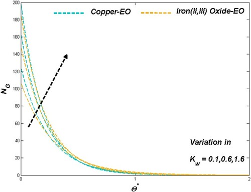
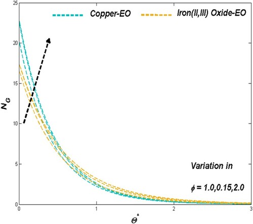
6.1. The effect of porous media parameter ${\mathit{K}}_{\mathit{w}}$

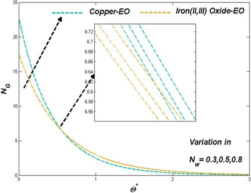
Porous media parameter $K_w$ sets the physical situation in favour of flow speed and thermal transport through the improving porosity nature of the medium employed in the modelled PTSC. Graphical presentations of Figures 6 and 7 proved the above-mentioned claim as the Darcian force acts behind as a key factor in such cases of Fe₃O₄-EO and Cu-EO combinations. Regarding thermal aspects of heat transfer rate along with the thermal boundary behaviour, the previous combination stays ahead of the other combination mentioned later may be due to its increased resistance from density hike for higher values of $K_w$. In these situations, the Cu-EO nanofluid seems more effective than Fe₃O₄-EO nanofluid (Figures 6 and 7). Drafts in Figure 8 disclosed the fact of entropy raise concerning the improved permeability which leads the heat transfer rate to decrease.

Figure 6. Velocity discrepancy versus $K_w$.

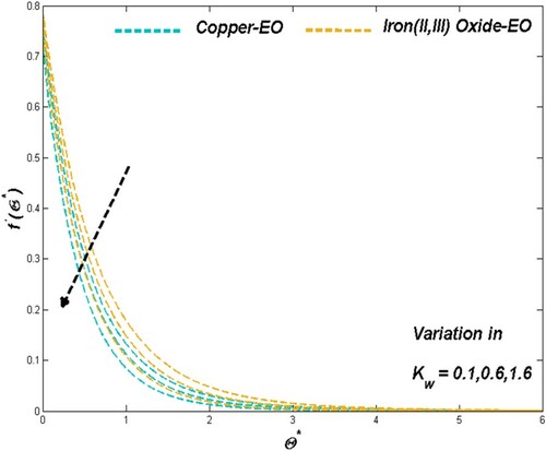
Figure 7. Temperature discrepancy versus $K_w$.

Figure 8. Entropy discrepancy versus $K_w$.

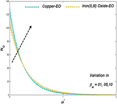
6.2 The effects of radiative parameter ${\mathit{N}}_{\mathit{w}}$ as well as variant thermal conductivity parameter $ϵ$

Figures 9 and 10 depict the complimenting fact of supplementary radiation heat towards the thermal dissemination and entropy formation for both Cu-EO and Fe₃O₄-EO nanofluids. As the add-on heat from the radiation provides the elevated workload to the fluid to drive away more from the system, it reflects in thermal dispersion and irreversible energy loss especially more for Cu-EO when compared to Fe₃O₄-EO nanofluids.

Figure 9. Temperature discrepancy versus $N_w$.

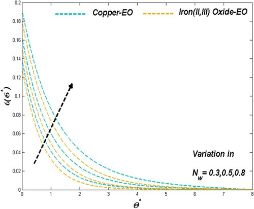
Figure 10. Entropy generation discrepancy versus $N_w$.

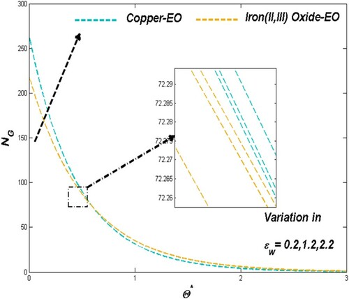
As the porosity constrain ϵ regulates the particle motion across the system, which acts in favour of thermal dispersion of Cu-EO nanofluid than that of Fe₃O₄-EO which can be evident through Figure 11. Figure 12 portrays the nominal but assisting contribution of porosity towards the irreversible energy loss.

Figure 11. Temperature discrepancy versus ${ϵ}_w$.

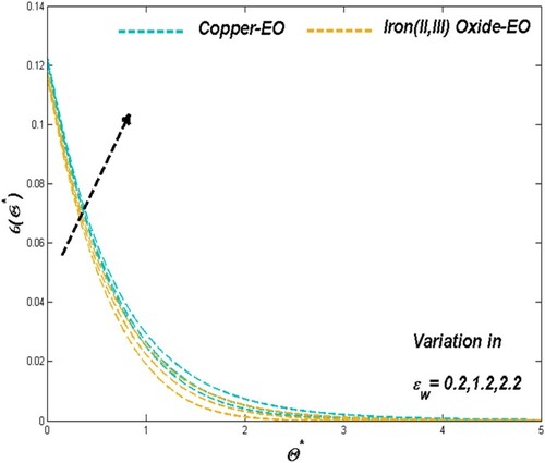
Figure 12. Entropy generation discrepancy versus ${ϵ}_w$.

6.3 The effect of Casson parameter ${\text{β}}_w$

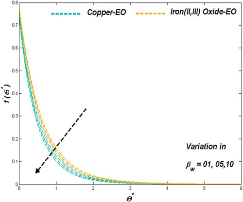
Improving Casson parameter ${\text{β}}_w$ represents the enhanced resistance towards the fluidity which reflects in the reduction of a velocity profile for both Cu-EO and Fe₃O₄-EO combination of fluids can be evident through Figure 13. Interestingly Cu-EO experienced more resistive effects than compared to the Fe₃O₄-EO nanofluid.

Figure 13. Velocity discrepancy versus ${\text{β}}_w$.

Corresponding to the resistive impact, the thermal dispersion by the slower fluid flow was in better form to drive away more heat from the surface. Figure 14 showcases the fact that the sluggish Cu-EO Casson nanoliquid combination drives more heat than the Fe₃O₄-EO combination.

Figure 14. Temperature discrepancy versus ${\text{β}}_w$.

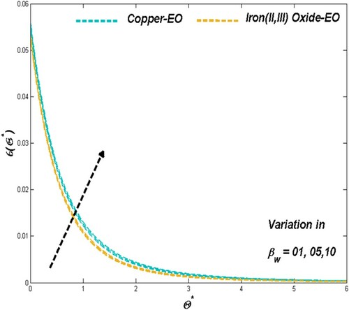
Figure 15 portrays the irreversible energy loss in the system for improving Casson constrain (${\text{β}}_w$). Though the impact seems nominal, the raising thermal transfer triggers to assist energy loss from it. Corresponding to the thermal transference the Fe₃O₄-EO Casson nanoliquid combination exerts more irreversible energy when compared to Cu-EO nanofluid.

Figure 15. Entropy discrepancy versus ${\text{β}}_w$.

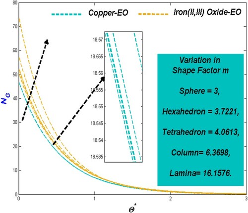
6.4 The effect of variation in nanoparticle shapes constraint m

As the shape of the suspending particle ranges from a sphere, hexahedron, tetrahedron, column to Lamina, the optimal choice has to be picked with respective flow situations. Figure 16 showcases the fact that the lamina particles exert better thermal disperse when compared to the hexahedron and spherical particles. Simultaneous escalation in the irreversible energy drain for particle shape variations can be observed from Figure 17 for both Cu-EO and Fe₃O₄-EO nanofluids.

Figure 16. Temperature discrepancies versus $m$.

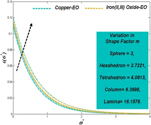
Figure 17. Entropy discrepancies versus $m$.

6.5 The consequence of nanoparticle size $\varphi$

Particle fraction reflects in the strength of the nanofluid towards its heat transference ability. As the improved particle suspension resists the fluidity, it provides the dual advantage for prompt thermal transference situations along with its thermal driving efficiency. Reduced fluidity and enhanced thermal dispersion from Figures 18 and 19 for both Cu-EO and Fe₃O₄-EO nanofluid justify the above claim. Thermal drive from the system simultaneously escalates the entropy formation for improved values of particle fraction can be observed in Figure 20.

Figure 18. Velocity Discrepancy Versus $\varphi$.

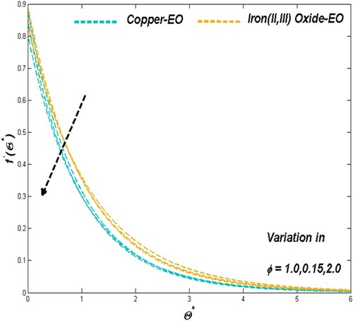
Figure 19. Temperature discrepancy versus $\varphi$.

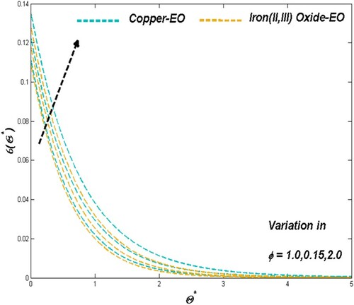
Figure 20. Entropy discrepancy versus $\varphi$.

6.6 The consequence of velocity slip ${\mathit{\Lambda }}_{\mathit{w}}$

Velocity slip constrain ${\mathrm{\Lambda }}_w$ acts against the fluidity of both Cu-EO and Fe₃O₄-EO nanofluid. Figure 21 reveals the fact that the fluid flow experienced some resistance through the particle suspension. As seen in the previous plots, Figure 22 is apparent the fact of slower fluidity and corresponding boost in the thermal dispersion. Interestingly, the irreversible energy loss gets reduced due to the nominal particle surface interaction which can be observed in Figure 23 for both Cu and Fe₃O₄ suspended engine oil-based nanofluids.

Figure 21. Velocity discrepancy versus ${\mathrm{\Lambda }}_w$.

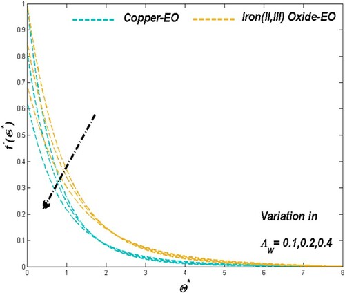
Figure 22. Temperature discrepancy versus ${\mathrm{\Lambda }}_w$.

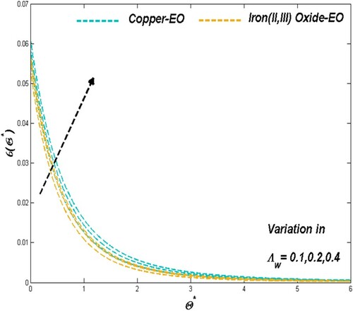
Figure 23. Entropy discrepancy versus ${\mathrm{\Lambda }}_w$.

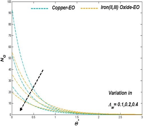
Figure 24. Temperature discrepancies versus $E_w$.

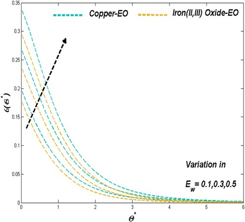
Figure 25. Entropy generation discrepancy versus $E_w$.

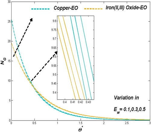
6.7 Impact of Eckert number ${\mathit{E}}_{\mathit{w}}$

For the Fe₃O₄-EO and the Cu-EO nanofluids, changes in the thermal and entropy for the Eckert numbers ($E_c$) have been reported in Figures 24 and Figure 25 correspondingly. The number of Eckert acts for thermal fluctuation and entropy in both circumstances. The fluid's internal friction combined with the platform's temperature improves the thermal condition of the liquids.

6.8 The parametrical influences on skin frictional factor

Among the two classes of nanofluids, the Cu-EO combination exerts more skin resistance than Fe₃O₄-EO nanofluids. From Table 3, it can be observed that the factors of Casson parameter and slip constrain tends to reduce the skin resistance by slows down the fluidity in the system. On other hand, parameters like magnetic constrain and fractional volume exhibits favourable situations for the particles to perform which elevates the frictional skin resistance.

Table 3. The value of skin resistance $=C_{f}R{e}_x^{\frac{1}{2}}$ and Nusselt number $=N_{u}R{e}_x^{\frac{-1}{2}}$ for $Pr=6450$.

${\text{β}}_w$	$M_w$	$K_w$	$\varphi$	${ϵ}_w$	${\mathrm{\Lambda }}_w$	$B_w$	$N_w$	$S$	$E_w$	$C_{f}R{e}_x^{\frac{1}{2}}$ Cu-EO	$C_{f}R{e}_x^{\frac{1}{2}}$ Fe3O4-EO	$N_{u}R{e}_x^{\frac{-1}{2}}$ Cu-EO	$N_{u}R{e}_x^{\frac{-1}{2}}$ Fe3O4-EO	Relative $\frac{N{u}_{\left(Cu\right)}-N{u}_{\left(F{e}_3{O}_4\right)}}{N{u}_{\left(Cu\right)}}\times 100$%
1.0	1.6	1.6	0.2	0.2	0.1	0.2	0.3	0.1	0.3	3.1100	2.7307	0.1442	0.1304	9.5%
5.0										2.3002	2.0315	0.1390	0.1293	6.9%
10.0										2.1831	1.9300	0.1350	0.1188	12.0%
	0.6									2.7898	2.3382	0.1502	0.1340	10.7%
	1.6									3.1100	2.7307	0.1442	0.1304	9.5%
	2.6									3.6288	3.3420	0.1332	0.1296	2.7%
		0.6								3.0820	2.5163	0.1512	0.1439	4.8%
		1.6								3.1100	2.7307	0.1442	0.1304	9.5%
		2.6								3.1415	3.7854	0.1217	0.1023	15.9%
			0.1							2.3877	2.1783	0.1824	0.1732	5.0%
			0.1							3.1100	2.7307	0.1442	0.1304	9.5%
			0.2							4.9206	4.2751	0.0906	0.0738	18.5%
				0.2						3.1100	2.7307	0.1442	0.1304	9.5%
				2.1						3.1100	2.7307	0.1420	0.1302	8.3%
				2.2						3.1100	2.7307	0.1380	0.1299	5.8%
					0.1					3.1100	2.7307	0.1442	0.1304	9.5%
					0.2					2.6164	2.3497	0.1410	0.1295	8.1%
					0.4					2.0063	1.8492	0.1330	0.1279	3.8%
						0.3				3.1100	2.7307	0.1442	0.1304	9.5%
						0.5				3.1100	2.7307	0.1388	0.1265	8.8%
						0.8				3.1100	2.7307	0.1207	0.1119	7.2%
							0.1			3.1100	2.7307	0.1371	0.1260	8.0%
							0.3			3.1100	2.7307	0.1442	0.1304	9.5%
							0.5			3.1100	2.7307	0.1625	0.1469	9.6%
								0.1		3.1100	2.7307	0.1442	0.1304	9.5%
								0.3		3.2947	2.8541	0.1578	0.1409	10.7%
								0.5		3.4868	2.9814	0.1622	0.1428	11.9%
									0.1	3.1100	2.7307	0.1284	0.1260	1.8%
									0.3	3.1100	2.7307	0.1442	0.1304	9.5%
									0.5	3.1100	2.7307	0.1798	0.1597	11.1%

6.9 Rate of thermal transference owing to the parametrical influences

Table 3 also displays the thermal transference rate in terms of Nusselt number for the parametrical impacts. Apart from the thermal radiation and S which creates the optimal thermal transference rate, all other constraints were looks to be against it. Comparatively, Cu suspended nanofluid exerts more thermal transference rate than the Fe₃O₄-EO nanofluid. Relative thermal transference gets hiked around 3% for Casson parameter and S constrain, 13% increase for particle fraction proportion. Nearly around 2% to 4% reduction in relative thermal transference rate can be evident for the parameters like a magnetic parameter, porosity, and Biot number.

7. Conclusions

Exploring the flow, thermal, and entropy formation aspects of Cu-EO and Fe₃O₄-EO Casson nanofluids over the Parabolic trough Solar Collector incorporated with the Magnetic influence with convective heated slippery flow under thermally radiation environment is considered. Results were plotted and reviewed in the form of graphs and tables. Some Key factors observed with the parametrical studies were listed below:

• Comparatively, Fe₃O₄-EO Casson nanofluid flows with better fluidity than the Cu-EO combination fluid

• Opposing nature towards the fluidity of the flow fluids was triggered by the factors of viscoelasticity, Lorentz force, particle fraction strength, and slip regime.

• In addition to the above-mentioned factors which set a favourable situation for thermal dispersion, the elements of thermal radiation heat and particle shape also exhibit improved thermal distribution in the system.

• Irreversible energy loss from the system can be regulated to a minimum with the physical aspects of viscoelasticity, magnetic influence, particle fraction, radiated heat, shape alterations of particle, convective heat, and Reynolds number. Interestingly, the slip factor stays a direct impact on screening the irreversibility.

• With the additional advantage of magnetic and particle fraction impacts, Cu-EO Casson nanofluid experiencing more skin resistance than the Fe₃O₄-EO class of fluid.

• Better thermal transference in terms of Nusselt number was found to be significant in Cu-EO than the Fe₃O₄-EO combination.

• As the magnetic parameter and Biot number around 3% of deduction in thermal transference rate, the nanoparticle fraction exerts around 13% on the favourable side.

Disclosure statement

No potential conflict of interest was reported by the author(s).

References

- Kreider JF, Kreith F. Solar energy handbook; 1981.
- Granqvist CG. Solar energy materials. Adv Mater. 2003;15(21):1789–1803.
- Ugli TJT. The importance of alternative solar energy sources and the advantages and disadvantages of using solar panels in this process. Int J Eng Inf Syst (IJEAIS). 2019;3(4):70–79.
- Tyagi H, Agarwal AK, Chakraborty PR, et al. Introduction to applications of solar energy. In: Applications of solar energy. Singapore: Springer; 2018. p. 3–10.
- Manikandan GK, Iniyan S, Goic R. Enhancing the optical and thermal efficiency of a parabolic trough collector–a review. Appl Energy. 2019;235:1524–1540.
- Fernández-García A, Zarza E, Valenzuela L, et al. Parabolic-trough solar collectors and their applications. Renew Sustain Energy Rev. 2010;14(7):1695–1721.
- Ahmed MS. Nanofluid: new fluids by nanotechnology. In: Thermophysical properties of complex materials. IntechOpen; 2019.
- Sheikhpour M, Arabi M, Kasaeian A, et al. Role of nanofluids in drug delivery and biomedical technology: methods and applications. Nanotechnol Sci Appl. 2020;13:47.
- Majumder SD, Das A. A short review of organic nanofluids: preparation, surfactants, and applications. Front Mater. 2021;8:1–8. Article No. 630182.
- Wong KV, De Leon O. Applications of nanofluids: current and future. Adv Mech Eng. 2010;2:519659.
- Dehaj MS, Rezaeian M, Mousavi D, et al. Efficiency of the parabolic through solar collector using NiFe2O4/water nanofluid and U-tube. J Taiwan Inst Chem Eng. 2021;120:136–149.
- Alashkar A, Gadalla M. Investigation of using ag/therminol nanofluids as heating fluids in PTSC-based power plants. In: ASME International Mechanical Engineering Congress and Exposition. American Society of Mechanical Engineers; 2017, November; Vol. 58417, p. V006T08A099.
- Richardson S. On the no-slip boundary condition. J Fluid Mech. 1973;59(4):707–719.
- Haq SU, Khan I, Ali F, et al. Influence of slip condition on unsteady free convection flow of viscous fluid with ramped wall temperature. In Abstract and applied analysis, Hindawi; 2015, August; Vol. 2015.
- Sayed HM, Aly EH, Vajravelu K. Influence of slip and convective boundary conditions on peristaltic transport of non-Newtonian nanofluids in an inclined asymmetric channel. Alexandria Eng J. 2016;55(3):2209–2220.
- Srinivasacharya D, Himabindu K. Effect of slip and convective boundary conditions on entropy generation in a porous channel due to micropolar fluid flow. Int J Nonlinear Sci Numer Simul. 2018;19(1):11–24.
- Acharya N, Das K, Kundu PK. Outlining the impact of second-order slip and multiple convective condition on nanofluid flow: a new statistical layout. Can J Phys. 2018;96(1):104–111.
- Siddiqui A, Shankar B. MHD flow and heat transfer of Casson nanofluid through a porous media over a stretching sheet. In: Kandelousi MS, Ameen S, Akhtar MS, et al., editors. Nanofluid flow in porous media. IntechOpen; 2019.
- Mukhopadhyay S. Casson fluid flow and heat transfer over a nonlinearly stretching surface. Chin Phys B. 2013;22(7):074701.
- Hayat T, Shehzad SA, Alsaedi A, et al. Mixed convection stagnation point flow of Casson fluid with convective boundary conditions. Chin Phys Lett. 2012;29(11):114704.
- Nawaz M, Hayat T, Alsaedi A. Dufour and Soret effects on MHD flow of viscous fluid between radially stretching sheets in porous medium. Appl Math Mech. 2012;33(11):1403–1418.
- Chamkha AJ, Aly AM. Heat and mass transfer in stagnation-point flow of a polar fluid towards a stretching surface in porous media in the presence of soret, Dufour and chemical reaction effects. Chem Eng Commun. 2010;198(2):214–234.
- Casson N. A flow equation for pigment-oil suspensions of the printing ink type. Rheology of disperse systems; 1959.
- Eid MR, Makinde OD. Solar radiation effect on a magneto nanofluid flow in a porous medium with chemically reactive species. Int J Chem Reactor Eng. 2018;16(9):1–14. Article No. 20170212.
- Mahanthesh B, Gireesha BJ, Gorla RS, et al. Magnetohydrodynamic three-dimensional flow of nanofluids with slip and thermal radiation over a nonlinear stretching sheet: a numerical study. Neural Comput Appl. 2018;30(5):1557–1567.
- Sekhar KR, Reddy GV, Raju CS, et al. Multiple slip effects on magnetohydrodynamic boundary layer flow over a stretching sheet embedded in a porous medium with radiation and joule heating. Spec Top Rev Porous Media: Int J. 2018;9(2):117–132.
- Sivaraj R, Banerjee S. Transport properties of non-Newtonian nanofluids and applications; 2021.
- Khater AH, Callebaut DK, Malfliet W, et al. Nonlinear dispersive Rayleigh–Taylor instabilities in magnetohydrodynamic flows. Phys Scr. 2001;64(6):533.
- Khater AH, Callebaut DK, Seadawy AR. Nonlinear dispersive instabilities in Kelvin–Helmholtz magnetohydrodynamic flows. Phys Scr. 2003;67(4):340.
- Khater AH, Callebaut DK, Helal MA, et al. Variational method for the nonlinear dynamics of an elliptic magnetic stagnation line. Eur Phys J D-At Mol Opt Plasma Phys. 2006;39(2):237–245.
- Seadawy AR. Stability analysis for two-dimensional ion-acoustic waves in quantum plasmas. Phys Plasmas. 2014;21(5):052107.
- Seadawy AR. Fractional solitary wave solutions of the nonlinear higher-order extended KdV equation in a stratified shear flow: part I. Comput Math Appl. 2015;70(4):345–352.
- Thumma T, Wakif A, Animasaun IL. Generalized differential quadrature analysis of unsteady three-dimensional MHD radiating dissipative Casson fluid conveying tiny particles. Heat Transfer. 2020;49(5):2595–2626.
- Abdelsalam SI, Bhatti MM. The study of non-Newtonian nanofluid with Hall and ion slip effects on peristaltically induced motion in a non-uniform channel. RSC Adv. 2018;8(15):7904–7915.
- Niu J, Fu C, Tan W. Slip-flow and heat transfer of a non-Newtonian nanofluid in a microtube. Plos one. 2012;7(5):e37274.
- Hayat T, Khan MI, Farooq M, et al. Impact of Cattaneo–Christov heat flux model in flow of variable thermal conductivity fluid over a variable thicked surface. Int J Heat Mass Transf. 2016;99:702–710.
- Abel MS, Mahesha N. Heat transfer in MHD viscoelastic fluid flow over a stretching sheet with variable thermal conductivity, non-uniform heat source and radiation. Appl Math Model. 2008;32(10):1965–1983.
- Sharma PR, Singh G. Effects of variable thermal conductivity and heat source/sink on MHD flow near a stagnation point on a linearly stretching sheet; 2009.
- Chiu CH. A decomposition method for solving the convective longitudinal fins with variable thermal conductivity. Int J Heat Mass Transf. 2002;45(10):2067–2075.
- Usman M, Hamid M, Zubair T, et al. Cu-Al2O3/Water hybrid nanofluid through a permeable surface in the presence of nonlinear radiation and variable thermal conductivity via LSM. Int J Heat Mass Transf. 2018;126:1347–1356.
- Lahmar S, Kezzar M, Eid MR, et al. Heat transfer of squeezing unsteady nanofluid flow under the effects of an inclined magnetic field and variable thermal conductivity. Physica A. 2020;540:123138.
- Irfan M, Khan M, Khan WA. Numerical analysis of unsteady 3D flow of Carreau nanofluid with variable thermal conductivity and heat source/sink. Results Phys. 2017;7:3315–3324.
- Mahian O, Kianifar A, Kleinstreuer C, et al. A review of entropy generation in nanofluid flow. Int J Heat Mass Transf. 2013;65:514–532.
- Roşca NC, Pop I. Hybrid nanofluids flows determined by a permeable power-Law stretching/shrinking sheet modulated by orthogonal surface shear. Entropy . 2021;23(7):813.
- Selimefendigil F, Öztop HF. Thermal management and modeling of forced convection and entropy generation in a vented cavity by simultaneous use of a curved porous layer and magnetic field. Entropy . 2021;23(2):152.
- Yang L, Du K, Zhang X. A theoretical investigation of thermal conductivity of nanofluids with particles in cylindrical shape by anisotropy analysis. Powder Technol. 2017;314:328–338.
- Oyelakin IS, Mondal S, Sibanda P. Unsteady Casson nanofluid flow over a stretching sheet with thermal radiation, convective and slip boundary conditions. Alex Eng J. 2016;55:1025–1035.
- Mukhopadhyay S, Vajravelu K, Gorder RAV. Casson fluid flow and heat transfer at an exponentially stretching permeable surface. J Appl Mech. 2013;80:054502–054502.
- Mustafa M, Khan JA. Model for flow of Casson nanofluid past a non-linearly stretching sheet considering magnetic field effects. AIP Adv. 2015;5:077148.
- Jamshed W. Numerical investigation of MHD impact on Maxwell nanofluid. Int Commun Heat Mass Transf. 2021;120:104973.
- Bhaskar N, Reddy P, Sreenivasulu P. Influence of variable thermal conductivity on MHD boundary layar slip flow of ethylene-glycol based CU nanofluids over a stretching sheet with convective boundary condition. J Eng Math. 2014: 1–10. Article No. 905158.
- Arunachalam R, Rajappa NR. Forced convection in liquid metals with variable thermal conductivityand capacity. ACTA MECH. 1978;31:25–31.
- Maxwell J. A treatise on electricity and magnesium. 2nd ed. Oxford: Clarendon Press; 1881.
- Xu X, Chen S. Cattaneo–Christov heat flux model for heat transfer of Marangoni boundary layer flow in a copper–water nanofluid. Heat Transfer Res. 2017;46:1281–1293.
- Jamshed W, Nisar KS, Ibrahim RW, et al. Computational frame work of Cattaneo-Christov heat flux effects on Engine Oil based williamson hybrid nanofluids: a thermal case study. Case Stud. Therm. Eng. 2021;26:101179.
- Jamshed W. Thermal augmentation in solar aircraft using tangent hyperbolic hybrid nanofluid: a solar energy application. Energy Environ. 2021;1–44. Article in press.
- Al-Hossainy AF, Eid MR. Combined theoretical and experimental DFT-TDDFT and thermal characteristics of 3-D flow in rotating tube of [PEG + H2O/SiO2-Fe3O4]C hybrid nanofluid to enhancing oil extraction. Waves Random Complex. 2021: 1–26. doi:https://doi.org/10.1080/17455030.2021.1948631.
- Jamshed W, Aziz A. A comparative entropy based analysis of Cu and Fe3O4 /methanol Powell-Eyring nanofluid in solar thermal collectors subjected to thermal radiation variable thermal conductivity and impact of different nanoparticles shape. Results Phys. 2018;9:195–205.
- Shahzad F, Jamshed W, Ibrahim RW, et al. Comparative numerical study of thermal features analysis between Oldroyd-B copper and molybdenum disulfide nanoparticles in engine-oil-based nanofluids flow. Coatings. 2021;11(10):1196.
- Brewster MQ. Thermal radiative transfer and properties. Hoboken (NJ): John Wiley and Sons; 1992.
- Keller HB. A New difference scheme for Parabolic problems. In: Hubbard B, editor. Numerical solutions of partial differential equations. New York: Academic Press; 1971. (vol. 2), p. 327–350.
- Sumalatha C, Bandari S. Effects of radiations and heat source/sink on a Casson fluid flow over nonlinear stretching sheet. WJM. 2015;5:257–265.
- Asif M, Jamshed W, Aziz A. Entropy and heat transfer analysis using Cattaneo-Christov heat flux model for a boundary layer flow of Casson nanofluid. Results Phys 2018;10:640–649.
- Jamshed W, Kumar V, Kumar V. Computational examination of Casson nanofluid due to a nonlinear stretching sheet subjected to particle shape factor: Tiwari and Das model. Numer Methods Partial Differ Equ. 2020; doi:https://doi.org/10.1002/num.22705.
- Ishak A, Nazar R, Pop I. Mixed convection on the stagnation point flow towards a vertical, continuously stretching sheet. J Heat Transf. 2007;129:1087–1090.
- Ishak A, Nazar R, Pop I. Boundary layer flow and heat transfer over an unsteady stretching vertical surface. Meccanica. 2009;44:369–375.
- Abolbashari MH, Freidoonimehr N, Nazari F, et al. Entropy analysis for an unsteady MHD flow past a stretching permeable surface in nanofluid. Adv Powder Tech. 2014;267:256–267.
- Das S, Chakraborty S, Jana RN, et al. Entropy analysis of unsteady magneto-nanofluid flow past accelerating stretching sheet with convective boundary condition. Appl Math Mech. 2015;36(2):1593–1610.