Interdecadal change in the South Asian summer monsoon rainfall in 2000 and contributions from regional tropical SST

ABSTRACT

The drying trend in the South Asian summer monsoon (SASM) area has been a focus of monsoon rainfall studies in the last two decades. However, this study reveals that a significant interdecadal change in the SASM rainfall occurred in approximately the year 2000. Obvious spatial inhomogeneity was a feature of this change, with increased rainfall over the southern part of the India–Pakistan border area that extends from the Arabian Sea, as well as in the western Bay of Bengal. Furthermore, there was decreased rainfall over the southern SASM and the western coast of the Indian Peninsula. Numerical experiments using CAM4 show that global SST changes can induce general changes in the SASM circulation consistent with observations. The tropical Pacific/Indian Ocean SST anomalies dominated the Walker and the regional Hadley circulation changes, respectively, while the descending motion anomalies over the southern SASM were further enhanced by the warmer tropical Atlantic SSTs. Moreover, the spatial inhomogeneity of this interdecadal change in the SASM rainfall needs further study.

Graphical abstract

摘要

本研究揭示，南亚夏季风降水在2000年左右发生了显著的年代际变化，主要表现为：印巴边境南部至阿拉伯海、孟加拉湾西部降水增加，而南部季风区和印度半岛西海岸降水减少。利用CAM4开展的海温敏感性试验显示，全球海温变化引起的季风环流变化与观测基本一致。热带太平洋和印度洋海温信号分别主导了Walker环流和局地Hadley环流变化，而热带大西洋海温则进一步增强了季风区南部的下沉运动异常。

KEYWORDS:

• South Asian summer monsoon
• Atlantic Multidecadal Oscillation
• Pacific Decadal Oscillation
• Indian Ocean SST
• summer rainfall

关键词:

• 南亚夏季风
• 大西洋多年代际涛动
• 太平洋年代际振荡
• 印度洋海温
• 夏季降水

1. Introduction

More than two billion people live in South Asia (5°–30°N, 60°–110°E), which is more than a quarter of the world’s population. Water resources management, agricultural production, and local economies greatly depend on the summer rainfall, which is dominated by the South Asian summer monsoon (SASM). The drying trend over India in the late twentieth century has been the focus of recent SASM studies. The increased concentrations of anthropogenic aerosols has been proposed to have played a prominent role in the weakening of the SASM in the past several decades (e.g. Bollasina, Ming, and Ramaswamy 2011). Although the all-India summer rainfall significantly decreased after the 1950s, century-long data reveal robust multidecadal variation (Turner and Annamalai 2012), with more rainfall during the 1880s–1890s, less during the 1900s–1920s, more during the 1930s–1950s, and less again since the 1950s.

The interdecadal variations in monsoon rainfall are robustly influenced by the SSTs in different regions. The Pacific Decadal Oscillation (PDO) can modulate the SASM and the monsoon–ENSO relationship (Krishnamurthy and Krishnamurthy 2014a, 2014b; Chakravorty, Gnanaseelan, and Pillai 2016). The warm/cold phase of the PDO is associated with a deficit/excess in rainfall over India. During warm PDO phases, the impact of El Niño/La Niña on rainfall is enhanced/reduced (Krishnamurthy and Krishnamurthy 2014b). The Atlantic Multidecadal Oscillation also modulates the SASM (e.g. Goswami et al. 2006; Luo, Li, and Furevik 2011; Luo et al. 2018) in combination with the PDO (e.g. Chakravorty, Gnanaseelan, and Pillai 2016; Malik et al. 2017). The tropical Indian Ocean SST can interact with the PDO and affect the monsoon rainfall (Chakravorty, Gnanaseelan, and Pillai 2016). At interannual timescales, ENSO is a major controlling mode (Shukla et al. 2011; Shukla and Kinter 2015). Warmer SST in the central-eastern tropical Pacific alters both the Walker and the regional Hadley circulation and influences the intensity and timing of monsoon activity. However, the ENSO–monsoon relationship is not stable (e.g. Krishnamurthy and Goswami 2000; Krishnamurthy and Krishnamurthy 2014b). The local SSTs, including the SSTs in the Arabian Sea and the Indian Ocean, also have an impact on the Indian summer monsoon (ISM) (e.g. Clark, Cole, and Webster 2000; Ashok, Guan, and Yamagata 2001; Konwar, Parekh, and Goswami 2012). Although previous studies have shown that SST changes in the Indian, Pacific and Atlantic oceans influence the SASM rainfall, the combined and independent contributions of these three regions are unclear.

Since the late 1990s, the PDO has transitioned from a positive to a negative phase (Zhu et al. 2011). At the same time, the East Asian summer monsoon, which significantly interacts with the SASM (e.g. Ding et al. 2013; Wu 2017; Wu, Hu, and Lin 2018), experienced interdecadal change with decreased and increased rainfall over the lower Yangtze River and the Huang–Huai River valley, respectively (e.g. Zhu et al. 2011, 2015; Liu et al. 2012). Therefore, it is natural to ask whether significant changes also occurred simultaneously in the SASM. To answer this question, we first examine the spatiotemporal characteristics of the ISM rainfall and find significant interdecadal changes appear in the SASM rainfall pattern after approximately the year 2000. Numerical experiments are then carried out using an atmospheric general circulation model (AGCM) to determine the possible impact of global SST changes.

2. Datasets and model experiments

The major datasets used in this study include the Global Precipitation Climatology Project (retrieved from https://www.esrl.noaa.gov/psd/), the National Centers for Environmental Prediction–National Center for Atmospheric Research reanalysis data on a 2.5° × 2.5° grid for the 39-yr period from 1979 to 2017 (Kalnay et al. 1996), and monthly mean SST data from the HadISST dataset from 1979 to 2017 with a horizontal resolution of 1° in both latitude and longitude (Rayner et al. 2003). Empirical orthogonal function (EOF) analyses were performed to extract the spatiotemporal structure of the South Asian rainfall.

In this study, we used the Community Atmosphere Model, version 4 (CAM4), with a horizontal resolution of 1° × 1° and 26 vertical hybrid levels. CAM4 is a widely used AGCM for diagnosing climate variations, and its ability to depict global and regional atmospheric circulation has been validated (e.g. Neale et al. 2013). Six sets of experiments were conducted: the control experiment (CTL simulation), in which the boundary condition was set as the model’s climatological monthly SST and sea ice, and five sensitivity experiments, in which the boundary condition was set as the SST anomalies between 2001–2017 and 1979–2000 (Figure S1) over the global/tropical/tropical Indian/tropical Pacific/tropical Atlantic Ocean (GA/TA/TIA/TPA/TAA simulation) imposed on the CTL simulation. A 30-year integration was run for each simulation. We analyzed the output data for the last 20 years, treating the first 10 years as the model’s spin-up period. The differences between the sensitivity and control simulations were compared with the observed changes to investigate the possible contributions of SST anomalies in different regions to the interdecadal shift in the SASM summer rainfall around the year 2000.

3. Results

Two kinds of indices are usually used to study the SASM: the regional mean monsoon rainfall and the regional mean circulation index (e.g. Webster and Yang 1992; Goswami, Krishnamurthy, and Annamalai 1999). The all-Indian summer rainfall is usually used to represent activity in the SASM. The simple regional mean index can represent the climate variation well if a strong regional homogeneity in the variable studied exists. However, the deficiency of the regional mean index is also obvious when robust spatial inhomogeneity is present at specific time scales because important information could be offset by calculating the regional mean. Therefore, we first investigate the spatiotemporal features of the SASM rainfall using EOF analysis.

3.1. Spatiotemporal features of the SASM rainfall

The EOF analysis was performed using the standardized monthly rainfall from South Asia (5°–30°N, 60°–110°E) from 1979 to 2017. The first three principal components explain 19.7%, 13.7%, and 10.4% of the total variance, respectively. The leading EOF mode (EOF1) exhibits a northwest–southeast-tilted dipole pattern, with positive anomalies over the Indian Peninsula centered over the western coast and negative anomalies over the northern Bay of Bengal (BOB) and the Indochina Peninsula. The time coefficients of EOF1 show strong interannual variability. The second EOF mode (EOF2) indicates a pattern with positive centers over the northern Indian Peninsula, the western Indian coast and the entire Indochina Peninsula, and negative anomalies over the northern Indian Ocean and the land area to the north of the BOB. The time coefficients also present robust interannual variations. The third EOF mode (EOF3) seems to exhibit a more complex spatial distribution, with negative anomalies over most areas in the Indian Peninsula and the eastern Arabian Sea, centered near the southern India–Pakistan border and the western BOB. Positive anomalies appear over the southern west coast of the Indian Peninsula, the southern edge of the Tibetan Plateau, and the western Indochina Peninsula. This pattern exhibits clear interdecadal variability and enters into a negative phase after approximately the year 2000 (Figure 1(f)).

Figure 1. The (a–c) spatial structures and (d–f) time coefficients of the first three EOF modes for the SASM rainfall during 1979–2017.

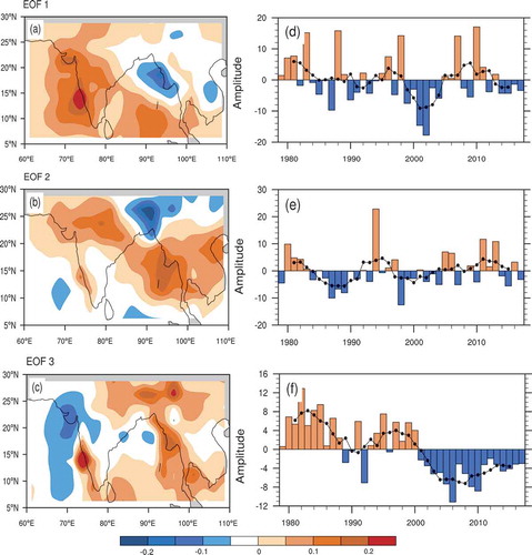
From the above EOF analyses, we can see distinct spatial inhomogeneity of the SASM rainfall. Therefore, we conclude that only weak or an absence of interdecadal variation can be obtained by evaluating the regional mean rainfall index from recent decades. The time series of EOF3, which explains 10.4% of the rainfall variance, shows a robust interdecadal change in approximately the year 2000 (deemed significant by a Mann–Kendall test). Therefore, we divided the whole period into 2001–2017 and 1979–2000 to explore the SASM-related changes to the regional and large-scale atmospheric circulation patterns and SSTs.

3.2. Interdecadal change in the regional atmospheric circulation after 2000

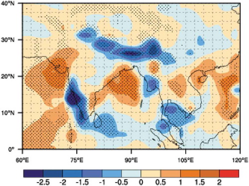
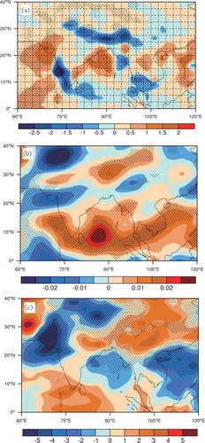
The difference in the summer mean rainfall between 1979–2000 and 2001–2017 shows a spatially heterogeneous pattern (Figure 2(a)). Positive anomalies are observed centered over the southern part of the India–Pakistan border, which extends over the eastern Arabian Sea and the Indian Ocean, as well as in the western BOB. Rainfall is mostly reduced over the ocean, with centers over the western Indian Peninsula and the southern tip of Southeast Asia. The strongest rainfall reduction mostly occurs over the Kerala along the western coast of India, where the monsoon onset is set as the arrival of the SASM (e.g. Taraphdar et al. 2018). The southern edge of the Tibetan Plateau is also occupied by depressed rainfall, which may be because the enhanced rainfall over the BOB leads to less moisture transport to the southern Tibetan Plateau. The vertical velocity at the 500 hPa level (Figure 2(b)) and outgoing longwave radiation (OLR, Figure 2(c)) show an overall pattern consistent with the changes in rainfall. Descending motion anomalies, represented by a positive vertical velocity, and OLR anomalies are revealed in the southern part of South Asia, mostly over the ocean. In addition, negative anomalies in the vertical motion and OLR are present in the northwestern Indian Peninsula and in the northeastern Arabian Sea, consistent with the ascending motion anomalies and increased rainfall observed in these regions. Although the OLR may represent ascending motion anomalies over the northern BOB, it cannot be captured by the vertical velocity in the reanalysis.

Figure 2. Difference in the (a) rainfall (units: mm) in south Asia, (b) 500-hPa omega (units: Pa s⁻¹), and (c) OLR (units: W m⁻²) between 2001–2017 and 1979–2000. Negative values in (b, c) represent ascending motion anomalies. Dotted areas are significant at the 90% confidence level based on the Student’s t-test.

3.3. Contributions of the global SST anomalies

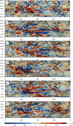
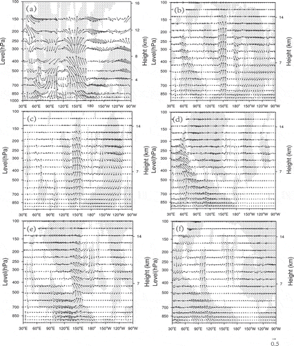
Observations of large-scale differences in the upper-level wind (Figures S2a and 3a) include strong westerly anomalies that appear over southern South Asia, which are related to the cyclonic anomalies over South Asia and the northwestern Pacific. These westerly anomalies appear to branch from the anticyclonic anomalies over northwestern Europe, which is part of the anomalous wave train pattern across Eurasia (e.g. Deng et al. 2018). In addition, strong westerly anomalies exist over the equatorial Pacific Ocean, with two anomalous cyclones in its south and north regions, reflecting a typical ENSO-related circulation pattern. However, in the lower-level circulation, the anomalous convergence was seen over the western coast of India and the Arabian Sea (Figure S2b), inconsistent with the dipole rainfall pattern (Figure 2(a)), which may suggest that the changes in the upper-level circulation could be major causes for this interdecadal change in the SASM rainfall. Therefore, we focus on the upper-level circulation in the following analysis.

The GA simulation (Figure 3b) can generally capture the westerly anomalies in the equatorial Pacific and the westerly anomalies over southern South Asia, which are related to the anomalous cyclones in that region. The increased rainfall over the Arabian Sea and the tropical Indian Ocean can also be reproduced. The largest discrepancy happens over the BOB and over southern East Asia: the simulated rainfall is negative in contrast to the observed positive rainfall anomalies. The TA simulation (Figure 3(c)) resembles the GA simulation. The TIA simulation (Figure 3(d)) can induce strong westerly anomalies over the eastern tropical Indian Ocean and cyclonic anomalies over the SASM and the northwestern Pacific. The TPA simulation (Figure 3(e)), however, has results in an overall rainfall pattern that are opposite to the TIA simulation, with increased rainfall over the southern SASM. The southerly anomalies in the TAA simulation (Figure 3(f)) over the eastern tropical Indian Ocean indicate anomalous local meridional circulation, with descending motion anomalies over SASM. Therefore, the tropical Indian Ocean SST dominates the rainfall and circulation changes in the SASM, which are strengthened by the tropical Atlantic SST and partly counteracted by the tropical Pacific SST.

Figure 3. (a) Difference in the large-scale wind at 200 hPa and precipitation (shading) in the observation between 1979–2000 and 2001–2017, and (b–f) difference in the model output between the GA/TA/TIA/TPA/TAA and CTL simulations. Dotted areas represent significant values in the precipitation at the 90% confidence level based on the Student’s t-test.

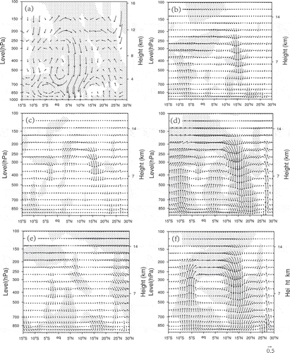
The Walker and regional Hadley circulation patterns are suggested to be important processes linking SSTs to the SASM (e.g. Krishnamurthy and Goswami 2000). We thus examine the changes in the Walker (averaged over 10°S–10°N) and regional Hadley (averaged over 75°–110°E) circulation in the observation and model results. In the Walker circulation after 2000 (Figure 4(a)), significant ascending motion anomalies appear over the western tropical Pacific and descending motion anomalies appear over the tropical eastern Pacific, although the latter are rather weak, which may be due to the relatively weak negative SST anomalies over the eastern tropical Pacific. Significant descending motion anomalies occur over the southern SASM and the eastern tropical Indian Ocean (approximately 75°–110°E), consistent with decreased rainfall in these regions. Ascending motion anomalies appear over the Arabian Sea and the eastern tropical Indian Ocean (approximately 60°–70°E), corresponding to the increased rainfall in these regions. The GA simulation (Figure 4(b)) can induce significant ascending motion anomalies over the western equatorial Pacific and weaker ones over the Arabian Sea and the western tropical Indian Ocean, along with weak descending motion anomalies over eastern tropical Indian Ocean (approximately 90°–110°E). The GA simulation is dominated by the TA simulation (Figure 4(c)). The ascending motion anomalies over the western tropical Pacific and descending motion anomalies over the eastern tropical Indian Ocean and the SASM are mostly captured by the TPA simulation (Figure 4(e)), while the ascending motion anomalies over the western tropical Indian Ocean are mostly captured in the TIA simulation (Figure 4(d)).

Figure 4. (a) Difference in the Walker circulation averaged over 10°S–10°N in the observation between 1979–2000 and 2001–2017, and (b–f) difference in the model output between the GA/TA/TIA/TPA/TAA and CTL simulations. Dotted areas represent significant values in the vertical or zonal wind velocity at the 90% confidence level based on the Student’s t-test.

Significant changes also occur in the regional Hadley circulation after 2000 (Figure 5(a)), including ascending motion anomalies near the equator and descending motion anomalies over 5°–15°N (consistent with the decreased rainfall in this region) and its southern counterpart. In the GA simulation (Figure 5(b)), ascending motion anomalies appear near the equator and descending motion anomalies appear over 5°–20°N, both of which are located more poleward than the observations. The signals in the TA (Figure 5(c)) simulation resemble those of the GA simulation quite closely, which are dominated by the TIA simulation (Figure 5(d)) and further strengthened by the TAA simulation (Figure 5(f)). The TPA simulation (Figure 5(e)) only contributes weakly to the regional Hadley circulation changes, opposite to the results of the TIA/TAA simulation.

Figure 5. (a) Difference in the regional Hadley circulation averaged over 75°–110°E in the observation between 1979–2000 and 2001–2017, and (b–f) difference in the model output between the GA/TA/TIA/TPA/TAA and CTL simulations. Dotted areas represent significant values in the vertical or meridional wind velocity at the 90% confidence level based on the Student’s t-test.

4. Summary

To investigate the decadal variation in the SASM, EOF analysis was performed to reveal the spatiotemporal structure of the monsoon rainfall. The third EOF mode shows significant interdecadal change after approximately the year 2000, with obvious spatial inhomogeneity, while the first two modes exhibit large interannual variation. The robust inhomogeneity of the SASM rainfall suggests the regional mean index is insufficient for studying variations in the SASM when used alone, which has long been practiced. The difference in the SASM rainfall and related circulation was then calculated to study the features of the interdecadal change after 2000. The results showed that, after 2000, the SASM rainfall exhibits significant spatially inhomogeneous changes, with negative anomalies over the southern SASM and the western coast of the Indian Peninsula, and positive anomalies over the Arabian Sea and the western tropical Indian Ocean, as well as in the BOB. An anomalous cyclone appears over South Asia at the upper level, with westerlies and easterlies dominating the southern and northern part.

An AGCM (CAM4) was used to diagnose the possible effect of global and regional SST changes in different tropical oceans on changes in the SASM. The global SST changes can capture the general features in the large-scale circulation over South Asia, especially the anomalous cyclone that is related to the westerly and easterly wind anomalies present in the southern and northern part in the upper level, respectively. The tropical SST forcing dominates the global SST effect, but with a somewhat weaker overall amplitude. In addition, the tropical Indian Ocean SST controls the tropical SST effect on the SASM, which is partly offset by the Pacific SST and strengthened by the Atlantic SST. For the Walker and regional Hadley circulation patterns, which are important in linking the tropical SST and the SASM, the tropical Pacific and Indian Ocean SSTs dominate the changes. It should be noted that calculations of regional Hadley circulation, which covers both positive and negative rainfall anomalies centers, can only depict the large-scale circulation, omitting signals at a finer scale.

Although CAM4 is somewhat capable of reproducing the overall circulation changes forced by SST changes, it is obviously deficient at simulating the spatial inhomogeneity of the SASM rainfall changes. Dynamical downscaling using regional climate models could be an effective way to reproduce such spatially inhomogeneous features of monsoon rainfall. Specifically, CAM4 cannot capture the increased rainfall over the BOB after 2000. This might be partly because the model cannot represent the monsoon depression activity well, and this activity greatly contributes to the rainfall over the BOB (e.g. Vishnu et al. 2016). Such an incapability in reproducing the monsoon rainfall is well known for state-of-the-art models, due to the models’ shortcomings in the cloud parameterization schemes (e.g. Sabeerali et al. 2015) and moisture transport (Sahana et al. 2019). Therefore, perfecting the models’ physical processes in depicting the rainfall formation should improve the models’ ability to portray monsoon precipitation. In addition, although we revealed the interdecadal change of the SASM rainfall around the year 2000, the reason for the spatial inhomogeneity is not yet clear and needs further study.

Disclosure statement

No potential conflict of interest was reported by the authors.

Supplementary material

Supplemental data for this article can be accessed here.

Additional information

Funding

This work was jointly supported by the National Key Research and Development Program of China [grant number 2017YFC1502304], the National Natural Science Foundation of China [grant numbers 41675083 and 41522503], and the Chinese Academy of Sciences–Peking University Joint Research Program.

References

- Ashok, K., Z. Guan, and T. Yamagata. 2001. “Impact of the Indian Ocean Dipole on the Relationship between the Indian Monsoon Rainfall and ENSO.” Geophysical Research Letters 28 (23): 4499–4502. doi:10.1029/2001gl013294.
- Bollasina, M. A., Y. Ming, and V. Ramaswamy. 2011. “Anthropogenic Aerosols and the Weakening of the South Asian Summer Monsoon.” Science 334 (6055): 502–505. doi:10.1126/science.1204994.
- Chakravorty, S., C. Gnanaseelan, and P. A. Pillai. 2016. “Combined Influence of Remote and Local SST Forcing on Indian Summer Monsoon Rainfall Variability.” Climate Dynamics 47 (9–10): 2817–2831. doi:10.1007/s00382-016-2999-5.
- Clark, C. O., J. E. Cole, and P. J. Webster. 2000. “Indian Ocean SST and Indian Summer Rainfall: Predictive Relationships and Their Decadal Variability.” Journal of Climate 13 (14): 2503–2519. doi:10.1175/1520-0442(2000)013<2503:Iosais>2.0.Co;2.
- Deng, K., S. Yang, M. Ting, A. Lin, and Z. Wang. 2018. “An Intensified Mode of Variability Modulating the Summer Heat Waves in Eastern Europe and Northern China.” Geophysical Research Letters 45 (20): 11361–11369. doi:10.1029/2018gl079836.
- Ding, Y., Y. Sun, Y. Liu, D. Si, Z. Wang, Y. Zhu, Y. Liu, et al. 2013. “Interdecadal and Interannual Variabilities of the Asian Summer Monsoon and Its Projection of Future Change.” Chinese Journal of Atmospheric Sciences 37 (2): 253–280.
- Goswami, B. N., V. Krishnamurthy, and H. Annamalai. 1999. “A Broad-scale Circulation Index for the Interannual Variability of the Indian Summer Monsoon.” Quarterly Journal of the Royal Meteorological Society 125 (554): 611–633. doi:10.1002/qj.49712555412.
- Goswami, B. N., M. S. Madhusoodanan, C. P. Neema, and D. Sengupta. 2006. “A Physical Mechanism for North Atlantic SST Influence on the Indian Summer Monsoon.” Geophysical Research Letters 33 (2): L02706. doi:10.1029/2005gl024803.
- Kalnay, E., M. Kanamitsu, R. Kistler, W. Collins, D. Deaven, L. Gandin, M. Iredell, et al. 1996. “The NCEP/NCAR 40-year Reanalysis Project.” Bulletin of the American Meteorological Society 77 (3): 437–471. doi:10.1175/1520-0477(1996)077<0437:tnyrp>2.0.co;2.
- Konwar, M., A. Parekh, and B. N. Goswami. 2012. “Dynamics of East-West Asymmetry of Indian Summer Monsoon Rainfall Trends in Recent Decades.” Geophysical Research Letters 39 (10): L10708. doi:10.1029/2012GL052018.
- Krishnamurthy, L., and V. Krishnamurthy. 2014a. “Decadal Scale Oscillations and Trend in the Indian Monsoon Rainfall.” Climate Dynamics 43 (1–2): 319–331. doi:10.1007/s00382-013-1870-1.
- Krishnamurthy, L., and V. Krishnamurthy. 2014b. “Influence of PDO on South Asian Summer Monsoon and Monsoon-ENSO Relation.” Climate Dynamics 42 (9–10): 2397–2410. doi:10.1007/s00382-013-1856-z.
- Krishnamurthy, V., and B. N. Goswami. 2000. “Indian Monsoon-ENSO Relationship on Interdecadal Timescale.” Journal of Climate 13 (3): 579–595. doi:10.1175/1520-0442(2000)013<0579:IMEROI>2.0.CO;2.
- Liu, H. W., T. J. Zhou, Y. X. Zhu, and Y. H. Lin. 2012. “The Strengthening East Asia Summer Monsoon since the Early 1990s.” Chinese Science Bulletin 57 (13): 1553–1558. doi:10.1007/s11434-012-4991-8.
- Luo, F., S. Li, and T. Furevik. 2011. “The Connection between the Atlantic Multidecadal Oscillation and the Indian Summer Monsoon in Bergen Climate Model Version 2.0.” Journal of Geophysical Research-Atmospheres 116: D19117. doi:10.1029/2011jd015848.
- Luo, F., S. Li, Y. Gao, L. Svendsen, T. Furevik, and N. Keenlyside. 2018. “The Connection between the Atlantic Multidecadal Oscillation and the Indian Summer Monsoon since the Industrial Revolution Is Intrinsic to the Climate System.” Environmental Research Letters 13 (9): 094020. doi:10.1088/1748-9326/aade11.
- Malik, A., S. Bronnimann, A. Stickler, C. C. Raible, S. Muthers, J. G. Anet, E. Rozanov, and W. Schmutz. 2017. “Decadal to Multi-decadal Scale Variability of Indian Summer Monsoon Rainfall in the Coupled Ocean-atmosphere-chemistry Climate Model SOCOL-MPIOM.” Climate Dynamics 49: 3551–3572. doi:10.1007/s00382-017-3529-9.
- Neale, R. B., J. Richter, S. Park, P. H. Lauritzen, S. J. Vavrus, P. J. Rasch, and M. Zhang. 2013. “The Mean Climate of the Community Atmosphere Model (CAM4) in Forced SST and Fully Coupled Experiments.” Journal of Climate 26 (14): 5150–5168. doi:10.1175/jcli-d-12-00236.1.
- Rayner, N. A., D. E. Parker, E. B. Horton, C. K. Folland, L. V. Alexander, D. P. Rowell, E. C. Kent, et al. 2003. “Global Analyses of Sea Surface Temperature, Sea Ice, and Night Marine Air Temperature since the Late Nineteenth Century.” Journal of Geophysical Research-Atmospheres 108 (D14): 4407. doi:10.1029/2002jd002670.
- Sabeerali, C. T., S. A. Rao, A. R. Dhakate, K. Salunke, and B. N. Goswami. 2015. “Why Ensemble Mean Projection of South Asian Monsoon Rainfall by CMIP5 Models Is Not Reliable?” Climate Dynamics 45 (1–2): 161–174. doi:10.1007/s00382-014-2269-3.
- Sahana, A. S., A. Pathak, M. K. Roxy, and S. Ghosh. 2019. “Understanding the Role of Moisture Transport on the Dry Bias in Indian Monsoon Simulations by CFSv2.” Climate Dynamics 52: 637–651. doi:10.1007/s00382-018-4154-y.
- Shukla, R. P., and J. L. Kinter. 2015. “Simulations of the Asian Monsoon Using a Regionally Coupled-global Model.” Climate Dynamics 44 (3–4): 827–843. doi:10.1007/s00382-014-2188-3.
- Shukla, R. P., K. C. Tripathi, A. C. Pandey, and I. M. L. Das. 2011. “Prediction of Indian Summer Monsoon Rainfall Using Nino Indices: A Neural Network Approach.” Atmospheric Research 102 (1–2): 99–109. doi:10.1016/j.atmosres.2011.06.013.
- Taraphdar, S., F. Zhang, L. R. Leung, X. Chen, and O. M. Pauluis. 2018. “MJO Affects the Monsoon Onset Timing over the Indian Region.” Geophysical Research Letters 45 (18): 10011–10018. doi:10.1029/2018gl078804.
- Turner, A. G., and H. Annamalai. 2012. “Climate Change and the South Asian Summer Monsoon.” Nature Climate Change 2: 587–595. doi:10.1038/nclimate1495.
- Vishnu, S., P. A. Francis, S. S. C. Shenoi, and S. S. V. S. Ramakrishna. 2016. “On the Decreasing Trend of the Number of Monsoon Depressions in the Bay of Bengal.” Environmental Research Letters 11 (1): 014011. doi:10.1088/1748-9326/11/1/014011.
- Webster, P. J., and S. Yang. 1992. “Monsoon and ENSO-Selectively Iteractive Systems.” Quarterly Journal of the Royal Meteorological Society 118 (507): 877–926. doi:10.1256/smsqj.50704.
- Wu, R. 2017. “Relationship between Indian and East Asian Summer Rainfall Variations.” Advances in Atmospheric Sciences 34 (1): 4–15. doi:10.1007/s00376-016-6216-6.
- Wu, R.-G., K.-M. Hu, and Z.-D. Lin. 2018. “Perspectives on the Non-stationarity of the Relationship between Indian and East Asian Summer Rainfall Variations.” Atmospheric and Oceanic Science Letters 11 (2): 104–111. doi:10.1080/16742834.2018.1387758.
- Zhu, Y., H. Wang, J. Ma, T. Wang, and J. Sun. 2015. “Contribution of the Phase Transition of Pacific Decadal Oscillation to the Late 1990s’ Shift in East China Summer Rainfall.” Journal of Geophysical Research-Atmospheres 120 (17): 8817–8827. doi:10.1002/2015jd023545.
- Zhu, Y., H. Wang, W. Zhou, and J. Ma. 2011. “Recent Changes in the Summer Precipitation Pattern in East China and the Background Circulation.” Climate Dynamics 36 (7–8): 1463–1473. doi:10.1007/s00382-010-0852-9.