Comparison of aircraft observations with ensemble forecast model results in terms of the microphysical characteristics of stratiform precipitation

ABSTRACT

The prediction of the particle number concentration and liquid/ice water content of cloud is significant for many aspects of atmospheric science. However, given the uncertainties in the initial and boundary conditions and imperfections of microphysical schemes, the accurate prediction of these microphysical properties of cloud is still a big challenge. The ensemble approach may be a viable way to reduce forecast uncertainties. In this paper, a large-scale stratiform cloud precipitation process is studied by comparing results of a 10-member ensemble forecast model with aircraft observation data. By means of the ensemble average, the prediction of bulk parameters such as liquid water content and ice water content can be improved in comparison with the control member, but the particle number concentrations are still one to two orders of magnitude less than those from observations. Intercomparison of raindrop size spectra reveals a big distinction between observations and predictions for particles with a diameter less than 1000 μm.

Graphical Abstract

摘要

云中的液态含水量, 冰水含量以及粒子数浓度在大气科学领域有着重要的作用。由于初边界条件的不确定性以及微物理方案的内在缺陷, 云中微物理特征的准确预报仍然是一大挑战。集合预报方法是减少预报不确定性的有效途径。本文使用10个集合成员与飞机观测资料进行对比研究太行山东麓一次大范围层状云降水过程。研究结果发现:与控制预报相比, 集合平均对液态含水量和冰水含量的预报能力有所提高, 然而粒子数浓度的预报与观测相比存在低估, 主要是因为模式低估了小于1000微米的降水粒子。

KEYWORDS:

• Aircraft observation
• ensemble forecast model
• particle number concentration
• liquid/ice water content

关键词:

• 飞机观测
• 集合模式
• 粒子数浓度
• 液态含水量/冰水含量

1. Introduction

Cloud properties, including cloud depth, liquid water content (LWC), ice water content (IWC), and particle number concentration, play important roles in climate change, large-scale synoptic systems, and local weather conditions due to their impacts on atmospheric radiation, energy balance, and precipitation efficiency (e.g., Sun and Shine 1995; Lohmann and Feichter 2005; Gettelman et al. 2012). Additionally, the vertical and horizontal distributions of LWC/IWC are also critical for cloud seeding (e.g., Dennis 1980).

Cloud observation using airborne instruments is an effective means to obtain the microphysical structure of clouds (e.g., McFarquhar and Black 2004; Lawson and Zuidema 2009). During recent decades, many field campaigns have been conducted in order to reveal the vertical structures of precipitation (e.g., Heymsfield et al. 2002; Field et al. 2005; Taylor et al. 2016). Vaillancourt et al. (2003) compared the 21 flights from the Canadian Freezing Drizzle Experiments with a mixed-phase cloud scheme model to evaluate the ability of the forecast system in terms of cloud phase and cloud water content. It was found that, in general, the model predicted ice clouds better than water clouds. Meanwhile, the model tended to overpredict the presence and quantities of IWC, and underpredict the supercooled liquid water. Zhang et al. (2007) compared the LWC from the Global Environmental Multiscale Model (GEM) with aircraft observations, and reported that although GEM reproduced the variation of LWC, the ‘in-cloud’ LWC values were generally overpredicted by the model using different resolutions. Hou et al. (2013) also found that the IWC simulated by the WRF model was larger than aircraft observations because of the predominant riming process.

However, these studies mentioned above are all based on single deterministic model results, which generally vary dramatically in terms of their initial and boundary conditions as well as parameterization schemes. Past research (e.g., Wolff and McDonough 2010; Thompson, Politovich, and Rasmussen 2017) has shown that cloudy regions predicted by single deterministic models tend to be smaller than observations. The uncertainties in the model’s initial and boundary conditions and imperfections in the model’s microphysical parameterizations will significantly influence the model results, and ensemble forecast modeling may improve the forecast capacity beyond any single forecast (Xu et al. 2019). Ensemble forecasts show great potential for quantitative precipitation forecasting. However, there are few studies on the prediction of cloud microphysics, such as LWC/IWC and number concentration, using ensemble forecasting. Furthermore, comparative studies between aircraft observations and ensemble numerical model results are even rarer.

In this paper, we utilize the Advanced Research version of the WRF model (ARW), version 3.6, including one control member and nine perturbation members, to simulate the process of stratiform precipitation induced by a cold front associated with an upper-level low-pressure trough that occurred on 21 May 2018 in Hebei Province, China. The LWC, IWC, and particle number concentrations obtained during two ascending and one horizontal flight at different altitudes are compared to the ensemble model results. The data are from the ‘Precipitation Enhancement and Hail Suppression in the Eastern Foothills of the Taihang Mountains’ experiment. The main purpose of the study is to expand the application of ensemble forecasting and evaluate the prediction ability of ensemble modeling to simulate cloud microphysical properties.

2. Data and model

2.1. Airborne instruments and flight track

On 21 May 2018, a large-scale stratiform precipitation event induced by a cold front associated with an upper-level low-pressure trough occurred in central and southern Hebei Province, China. Moderate to heavy rain appeared at the eastern foothills of the Taihang Mountains. In order to investigate the microphysical properties of this mesoscale precipitation system and evaluate the effects of cloud seeding, an aircraft observation experiment was conducted in this region. The airborne particle measurement system used in our study consisted of a cloud imaging probe (CIP), a high-volume precipitation spectrometer (HVPS), a cloud particle imager probe (CPI), a Nevzorov liquid water content probe (LWC), a Nevzorov total water content probe (TWC), and an aircraft-integrated meteorological measurement system (AIMMS20). Detailed information on each probe is provided in Table 1. Specially designed tips on the arms of the 2D probes were utilized to avoid the particle shattering issue (Korolev and Isaac 2005), while only particles greater than 100 μm were taken into account because of the inaccuracy of the depth of field for diameters less than 100 μm in size (Baumgardner and Korolev 1997). In order to include all small and large particles with diameters from submillimeters to centimeters, the cutoff size between CIP and HVPS was set to 900 μm. The particle number concentrations measured by CIP and HVPS did not include the contribution from cloud droplets because the range of the instruments was 100–8700 μm. The IWC value was calculated by total water content (TWC) minus LWC. The Nevzorov TWC probe measurements were calculated from the measurements of power used for the melting and evaporation of ice particles impacting the surface of a heated hot-wire sensor, but some of the ice particles—especially large particles—may rebound off the TWC cone into the airstream and be swept away, which may result in an underestimated measurement of the IWC, with the errors ranging from 10% to 20% (e.g., Korolev et al. 2013). At 1937 LST, the aircraft departed from Shijiazhuang airport, experienced a spiral ascent and horizontal flight, and then landed at 2337 LST.

Table 1. Summary of instruments and parameters used in this study.

Instrument	Manufacturer	Range	Resolution	Application
CIP	DMT	25–1550 μm	25 μm	Cloud droplets
HVPS	SPEC	150–8700 μm	150–750 μm	Precipitation particles
CPI	SPEC	10–2000 μm	2.3 μm	Images of cloud droplets, ice crystals, raindrops
LWC	Nevzorov	0–3 g m^−3		Liquid water content
TWC	Nevzorov	0–3 g m^−3		Total water content
AIMMS-20	DMT			Temperature, pressure, humidity, wind velocity

2.2. Model configuration

In this study, an ensemble forecast with 10 members was utilized to simulate this precipitation event. For the control member (C00), the initial and boundary conditions were provided by the high-resolution predictions of the National Centers for Environmental Prediction (NCEP) Global Forecast System, while for the nine members (C01–C09), the perturbations of the initial and boundary conditions were extracted from the high-resolution predictions of the NCEP Global Ensemble Forecast System (GEFS). GEFS attempts to quantify the amount of uncertainty in a forecast by generating an ensemble of multiple forecasts, with each perturbation from EnKF analysis (Zhou et al. 2016, 2017). The physical parameterization schemes used in each member are summarized in Table 2. The ensemble forecast with 10 members used different initial and boundary conditions, surface layer schemes, and planetary boundary layer physics schemes, and all members used the Morrison cloud microphysics scheme, which predicts the bulk parameters and size distributions of different particles (e.g., rain, ice, snow, and graupel) simultaneously. We chose this cloud microphysics scheme because it has been extensively tested and compared with both idealized and real case studies covering a wide range of conditions. RRTMG longwave and shortwave radiation schemes were used (Iacono et al. 2008), while the cumulus convection parameterization schemes were turned off. The simulation time was from 0600 UTC to 1800 UTC 21 May 2018 and the number of grids was 300 × 300, with a 3-km horizontal resolution and 50 eta (η) levels used in the vertical direction.

Table 2. Model configuration.

Member	Surface layer scheme	Planetary boundary layer physics scheme
C00	CLM4	YSU
C01	CLM4	MYNN2
C02	NOAH	YSU
C03	RUC	YSU
C04	NOAH	YSU
C05	CLM4	MYNN2
C06	NOAH	MYNN2
C07	RUC	MYNN2
C08	CLM4	YSU
C09	NOAH	YSU

3. Results

3.1. Six-hour cumulative precipitation and flight track of the aircraft

The 6-h cumulative precipitation from 1200 to 1800 UTC, which was also the flight time of the observation, of the control member (C00) and observation is shown in Figure 1(a,b). The results illustrate that the simulated precipitation band overlaps over Shanxi Province, Hebei Province, and Beijing from west to east, and the precipitation distribution is very similar with the observation. The precipitation in the eastern foothills of the Taihang Mountains is larger than that in the surrounding region due to the influence of topography. Moreover, although the 6-h cumulative precipitation of the control member is less than that of the observation, the main structure of this surface precipitation is roughly reproduced by the control member.

Figure 1. Six-hour accumulated precipitation of (a) the control member (C00) and (b) the observation; six-hour accumulated precipitation (c) in the aircraft observation region of the control member (C00) and (d) in the flight track region of the observation. The red line represents the flight track of the aircraft. The black rectangle represents three regions: AB, CD, and EF. The black annotations in (c, d) are the times of the flight observation. The hourly 0.1° gridded precipitation dataset resulting from the fusion of China’s automated stations and CMORPH is used as the observation data.

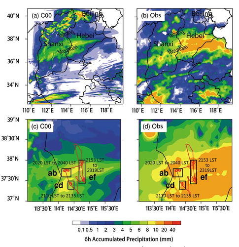
Figure 1(c,d) demonstrates the regions of the aircraft observations and flight path. The aircraft performed two processes of spiral observation, AB and CD, during 2020–2040 LST and 2110–2135 LST, respectively. A horizontal flight performed at different altitudes, EF, during 2153–2319 LST, was also performed.

The model results are averaged over three regions, where the aircraft observations were performed, as indicated by the black rectangle in Figure 1(c,d). The observation data are divided into two stages: the spiral ascent stage and horizontal flight stage. The average and median values of every 500 m are taken in the spiral ascent stage, and the average and median values of each altitude layer are taken in the horizontal flight stage to reduce random errors due to the small sample volume of airborne probes (Fleishauer, Larson, and Vonder Haar 2002). In this paper, we compare the observational and predicted cloud microphysical characteristics in the AB, CD, and EF regions.

3.2. Microphysical characteristics of region AB

Figure 2 demonstrates the vertical distributions of LWC, IWC, and particle number concentration from the observation and ensemble model in region AB. It shows that the results of the average values (every 500 m) are slightly larger than or similar to the results of the median values (every 500 m). The observation values below are taken as the average values. It can be seen that the observed LWC has a value of 0.07 g m⁻³ at 4350 m, while the value of LWC simulated by the ensemble average and control member is 0.12 g m⁻³ at 4063 m and 0.17 g m⁻³ at 3578 m, respectively (Figure 2(a)). The height of the peak value of LWC is near the height of the 0°C isotherm (about 4400 m), regardless of observation or model simulation. The simulation result of the ensemble-averaged LWC is closer to the observation compared with the control member. Similarly, the simulation result of the ensemble average is better than the control member for IWC (Figure 2(b)). It can be seen that the observed IWC has a value of 0.22 g m⁻³ at 4350 m, while the value of IWC simulated by the ensemble average is 0.3 g m⁻³ at 4590 m. However, the IWC simulated by the control member is larger, with a value of 0.65 g m⁻³ at 4550 m. The height of the peak value of IWC is also near the height of the 0°C isotherm. The ice particles falling from the upper layer are not completely melted in this height layer, and the habits of the particles are predominated by needles, aggregates, and irregular small ice particles (Figure 2(d)). The processes of riming and melting may result in the peak value of LWC/IWC. It should be noted that the TWC probe is very sensitive, so the partly melted ice particles are classified into IWCs below the melting layer. This may result in observational uncertainty within the melting layer and may carry some errors.

Figure 2. (a) Vertical distributions of LWC in region AB. The blue line represents the LWC from the control member (C00). The light gray line represents the LWC from the nine perturbation members (C01–C09). The red line is the ensemble average. The black line represents the result of the observation (average values of every 500 m) and the standard deviations at both ends. The green line represents the result of the observation (median values of every 500 m) and the standard deviations at both ends. (b) As in (a) but for IWC. (c) As in (a) but for ice and rain particle number concentration. (d) High-resolution particle image from CPI at different heights.

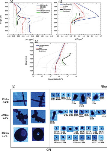
Overall, although the simulation results of the nine perturbation members (C01–C09) are quite different, reflecting the effects of uncertainty in the initial field on the cloud microphysics, the ensemble-average results are better than those of the control member, and the simulation ability for IWC is better than that for LWC.

Figure 2(c) reveals the vertical distributions of particle number concentration from the observation and ensemble model in region AB. Regardless of whether for the ensemble average or control member, the simulated particle number concentrations are one to two orders of magnitude less than those from observations. The possible reasons are as follows: The cloud microphysical scheme adopted by the ensemble forecast model is the Morrison scheme (Morrison, Thompson, and Tatarskii 2009), which has a constant droplet number concentration. The uncertainty of the cloud microphysical scheme (e.g., the method of setting the constant droplet number concentration and the nucleation scheme for ice crystals) may result in inaccurate prediction of the number concentration.

3.3. Microphysical characteristics of region CD

The vertical distributions of the LWC, IWC, and particle number concentration from the observation and ensemble model in region CD are demonstrated in Figure 3. The results show that the observed LWC has a value of 0.06 g m⁻³ at 4550 m, while the value of LWC simulated by the ensemble average and control member is 0.2 g m⁻³ at 3856 m and 0.33 g m⁻³ at 3856 m (Figure 3(a)), respectively. The model overestimates LWC compared with observations. The value of IWC in region CD is smaller than that in region AB, whether in the observation or simulation. The vertical distributions of IWC in CD from the Nevzorov IWC probe and model are very similar. For instance, the observed IWC reaches a value of 0.19 g m⁻³ at 4531 m, while the value of IWC simulated by the ensemble average and control member is 0.2 g m⁻³ at 4837 m and 0.27 g m⁻³ at 4345 m, respectively (Figure 3(b)). Compared with the control member, the result of the ensemble average is closer to the observation, and the simulation result for IWC is better than for LWC based on the ensemble average.

Figure 3. (a) Vertical distributions of LWC in region CD. The blue line represents the LWC from the control member (C00). The light gray line represents the LWC from the nine perturbation members (C01–C09). The red line is the ensemble average. The black line represents the result of the observation (average values of every 500 m) and the standard deviations at both ends. The green line represents the result of the observation (median values of every 500 m) and the standard deviations at both ends. (b) As in (a) but for IWC. (c) As in (a) but for ice and rain particle number concentration. (d) High-resolution particle image from CPI at different heights.

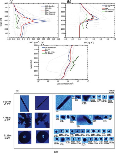
From the CPI particle image (Figure 3(d)), it can be seen that the ice particles in the colder part of the cloud are mainly small-scale ice particles produced by the deposition process, compared with region AB. Similar to region AB, the habits of the particles are predominated by aggregates and some lightly rimed ice particles at about the height of the 0°C isotherm (Figure 3(d)), and the ensemble model underestimates the particle number concentration regardless of whether the ensemble average or control member (Figure 3(c)).

3.4. Microphysical characteristics of region EF

Figure 4 shows the vertical distributions of cloud microphysical characteristics from the horizontal flight (EF), in which observations were performed at altitudes of 5600, 5100, 4800, 4300, 3600, 3000, 2400, and 2100 m. The results demonstrate that the averages in a wide range of temporal and spatial scales of region EF are better than those of the ascent spiral stage (regions AB and CD).

Figure 4. (a) Vertical distributions of LWC in region EF. The blue line represents the LWC from the control member (C00). The light gray line represents the LWC from the nine perturbation members (C01–C09). The red line is the ensemble average. The black line represents the result of the observation (average values at altitudes of 5600, 5100, 4800, 4300, 3600, 3000, 2400, and 2100 m) and the standard deviations at both ends. The green line represents the result of the observation (median values at altitudes of 5600, 5100, 4800, 4300, 3600, 3000, 2400, and 2100 m) and the standard deviations at both ends. (b) As in (a) but for IWC. (c) As in (a) but for ice and rain particle number concentration. (d) High-resolution particle image from CPI at different heights.

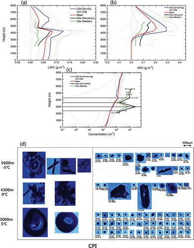
Compared with the control member, the result of the ensemble average is much better. The observed and ensemble-average value of LWC is 0.07 and 0.08 g m⁻³ at about 4300 m, respectively (Figure 4(a)). The ensemble-average results of IWC are also better in comparison with the control member, especially at the height above the 0°C isotherm. The observed and ensemble-average simulated value of IWC is 0.15 and 0.2 g m⁻³ at 4800 m, respectively (Figure 4(b)). Similar to Figures 2 and 3, regardless of whether for the ensemble average or control member, the simulated particle number concentrations are one or two orders of magnitude less than those from observations (Figure 4(c)).

During the EF stage, the habits of the particles are related to the temperature (Figure 4(d)). For instance, column and plate ice crystals dominate the colder part of the cloud (approximately −5°C) and the warmer layer (approximately 0°C) is dominated by aggregates and some lightly rimed ice particles.

3.5. Particle size distributions of raindrops

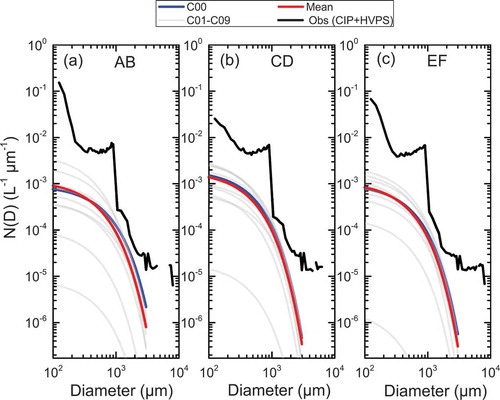
Figure 5 demonstrates the particle size distributions of raindrops from the model results and airborne instruments in regions AB, CD, and EF in the lower parts of the cloud (2400 m, 6.3°C). The results show that the number concentrations of raindrops with diameters greater than 1000 μm are close to the observations, and the control member and ensemble average are similar to each other. The predictions of the particle number concentrations of raindrops with diameters below 1000 μm are one to two orders of magnitude less than in the observations. The inaccurate prediction of the number concentration of small particles may be due to the uncertainties of the cloud microphysical scheme, including the method of assuming a constant droplet number concentration, as well as the ice nucleation scheme without consideration of the aerosol process, which can both lead to underestimation of the number concentration.

Figure 5. (a) Particle size distribution of raindrops for AB region (2400 m, 6.3°C). The blue line represents the control member (C00). The light gray line represents nine perturbation members (C01–C09). The red line represents the ensemble average. The black line represents the observation. (b) The same as (a), but for CD region. (c) The same as (a), but for EF region.

4. Conclusions

This paper compares the observed LWC, IWC, and particle number concentration of two ascending and one horizontal flight to ensemble model results, in order to evaluate the prediction ability of the ensemble model. The findings can be summarized as follows:

1. By disturbing the initial and boundary conditions without changing the cloud microphysics scheme, the simulation result of the ensemble average is much better than that of the control forecast in terms of bulk parameters (i.e., IWC, LWC, and number concentration). However, it should be noted that the prediction of particle number concentration is still one to two orders of magnitude less than observed due to the uncertainty of the cloud microphysical scheme (e.g., the constant droplet number concentration and the ice nucleation scheme), which result in a big distinction between observations and predictions for particles with diameters less than 1000 μm.

2. In general, although the ensemble-average approach is more accurate for the simulation of bulk parameters in terms of IWC and LWC in spiral ascent stages, the simulation results from the horizontal flight stage are even better, indicating that the average of model results over larger temporal and spatial scales can be closer to the observation.

3. In this case, high-resolution images from the CPI probe demonstrate that the habits of particles are closely related to the temperature. For instance, needle, column, and plate ice crystals dominate the colder part of the cloud (approximately −5°C), and the supercooled water layer in the warmer parts of the cloud (approximately 0°C) is dominated by aggregates and lightly rimed ice particles due to the riming process.

We also note that, due to the uncertainties of the cloud microphysical processes, more detailed schemes, such as spectral bin microphysics scheme, as well as aerosol-aware models, need to be tested using the ensemble approach for comparison with observations in the future. Moreover, aircraft observations only cover a small portion of the clouds due to the limitation of flight altitude, so more data obtained in deeply developed weather systems should also be utilized to compare with ensemble forecast models. Besides, all the conclusions reached in this paper are based on a single case study; more studies are needed in the future to better evaluate the capability of ensemble forecasting in modeling cloud microphysics.

Disclosure statement

No potential conflict of interest was reported by the authors.

Supplementary material

Supplemental data for this article can be accessed here.

Additional information

Funding

This work was supported by the National Key R&D Program of China [grant number 2018YFC1507900] and the Demonstration Project of Artificial Precipitation Enhancement and Hail Suppression Operation Technology at the Eastern Side of the Taihang Mountains [grant number hbrywcsy-2017-2], and was sponsored by the National Natural Science Foundation of China [grant numbers 41530427 and 41875172].

References

- Baumgardner, D., and A. Korolev. 1997. “Airspeed Corrections for Optical Array Probe Sample Volumes.” Journal of Atmospheric and Oceanic Technology 14 (5): 1224–1229. doi:10.1175/1520-0426(1997)014<1224:ACFOAP>2.0.CO;2.
- Dennis, A. S. 1980. Weather Modification by Cloud Seeding. London: Academic Press.
- Field, P. R., R. J. Hogan, P. R. A. Brown, A. J. Illingworth, T. W. Choularton, and R. J. Cotton. 2005. “Parametrization of Ice-particle Size Distributions for Mid-latitude Stratiform Cloud.” Quarterly Journal of the Royal Meteorological Society: A Journal of the Atmospheric Sciences, Applied Meteorology and Physical Oceanography 131 (609): 1997–2017. doi:10.1256/qj.04.134.
- Fleishauer, R. P., V. E. Larson, and T. H. Vonder Haar. 2002. “Observed Microphysical Structure of Midlevel, Mixed-phase Clouds.” Journal of the Atmospheric Sciences 59 (11): 1779–1804. doi:10.1175/1520-0469(2002)059<1779:OMSOMM>2.0.CO;2.
- Gettelman, A., X. Liu, D. Barahona, U. Lohmann, and C. Chen. 2012. “Climate Impacts of Ice Nucleation.” Journal of Geophysical Research: Atmospheres 117 (D20). doi:10.1029/2012JD017950.
- Heymsfield, A. J., A. Bansemer, P. R. Field, S. L. Durden, J. L. Stith, J. E. Dye, W. Hall, et al. 2002. “Observations and Parameterizations of Particle Size Distributions in Deep Tropical Cirrus and Stratiform Precipitating Clouds: Results from in Situ Observations in TRMM Field Campaigns.” Journal of the Atmospheric Sciences 59 (24): 3457–3491. DOI:10.1175/1520-0469(2002)059<3457:OAPOPS>2.0.CO;2.
- Hou, T. J., H. C. Lei, Z. X. Hu, and Q. J. Feng. 2013. “Observations and Modeling of Ice Water Content in a Mixed-phase Cloud System.” Atmospheric and Oceanic Science Letters 6 (4): 210–215. doi:10.3878/j.issn.1674-2834.13.0020.
- Iacono, M. J., J. S. Delamere, E. J. Mlawer, M. W. Shephard, S. A. Clough, and W. D. Collins. 2008. “Radiative Forcing by Long‐lived Greenhouse Gases: Calculations with the AER Radiative Transfer Models.” Journal of Geophysical Research: Atmospheres 113 (D13). doi:10.1029/2008JD009944.
- Korolev, A., and G. A. Isaac. 2005. “Shattering during Sampling by OAPs and HVPS. Part I: Snow Particles.” Journal of Atmospheric and Oceanic Technology 22 (5): 528–542. doi:10.1175/JTECH1720.1.
- Korolev, A., J. W. Strapp, G. A. Isaac, and E. Emery. 2013. “Improved Airborne Hot-wire Measurements of Ice Water Content in Clouds.” Journal of Atmospheric and Oceanic Technology 30 (9): 2121–2131. doi:10.1175/JTECH-D-13-00007.1.
- Lawson, R. P., and P. Zuidema. 2009. “Aircraft Microphysical and Surface-based Radar Observations of Summertime Arctic Clouds.” Journal of the Atmospheric Sciences 66 (12): 3505–3529. doi:10.1175/2009JAS3177.1.
- Lohmann, U., and J. Feichter. 2005. “Global Indirect Aerosol Effects: A Review.” Atmospheric Chemistry and Physics 5 (3): 715–737. doi:10.5194/acp-5-715-2005.
- McFarquhar, G. M., and R. A. Black. 2004. “Observations of Particle Size and Phase in Tropical Cyclones: Implications for Mesoscale Modeling of Microphysical Processes.” Journal of the Atmospheric Sciences 61 (4): 422–439. doi:10.1175/1520-0469(2004)061<0422:OOPSAP>2.0.CO;2.
- Morrison, H., G. Thompson, and V. Tatarskii. 2009. “Impact of Cloud Microphysics on the Development of Trailing Stratiform Precipitation in a Simulated Squall Line: Comparison of One-and Two-moment Schemes.” Monthly Weather Review 137 (3): 991–1007. doi:10.1175/2008MWR2556.1.
- Sun, Z., and K. P. Shine. 1995. “Parameterization of Ice Cloud Radiative Properties and Its Application to the Potential Climatic Importance of Mixed-phase Clouds.” Journal of Climate 8 (7): 1874–1888. doi:10.1175/1520-0442(1995)008<1874:POICRP>2.0.CO;2.
- Taylor, J. W., T. W. Choularton, A. M. Blyth, Z. Liu, K. N. Bower, J. Crosier, M. W. Gallagher, et al. 2016. “Observations of Cloud Microphysics and Ice Formation during COPE.” Atmospheric Chemistry and Physics 16 (2): 799–826. DOI:10.5194/acp-16-799-2016.
- Thompson, G., M. K. Politovich, and R. M. Rasmussen. 2017. “A Numerical Weather Model’s Ability to Predict Characteristics of Aircraft Icing Environments.” Weather and Forecasting 32 (1): 207–221. doi:10.1175/WAF-D-16-0125.1.
- Vaillancourt, P. A., A. Tremblay, S. G. Cober, and G. A. Isaac. 2003. “Comparison of Aircraft Observations with Mixed-phase Cloud Simulations.” Monthly Weather Review 131 (4): 656–671. doi:10.1175/1520-0493(2003)131<0656:COAOWM>2.0.CO;2.
- Wolff, C., and F. McDonough. 2010. “A Comparison of WRF-RR and RUC Forecasts of Aircraft Icing Conditions.” 14th Conference on Aviation, Range, and Aerospace Meteorology. Atlanta, GA: America Meteor.
- Xu, M., G. Thompson, D. R. Adriaansen, and S. D. Landolt. 2019. “On the Value of Time-Lag-Ensemble Averaging to Improve Numerical Model Predictions of Aircraft Icing Conditions.” Weather and Forecasting 34 (3): 507–519. doi:10.1175/WAF-D-18-0087.1.
- Zhang, J., W. Gong, W. R. Leaitch, and J. W. Strapp. 2007. “Evaluation of Modeled Cloud Properties against Aircraft Observations for Air Quality Applications.” Journal of Geophysical Research: Atmospheres 112 (D10). doi:10.1029/2006JD007596.
- Zhou, X., Y. Zhu, D. Hou, and D. Kleist. 2016. “A Comparison of Perturbations from an Ensemble Transform and an Ensemble Kalman Filter for the NCEP Global Ensemble Forecast System.” Weather and Forecasting 31 (6): 2057–2074. doi:10.1175/WAF-D-16-0109.1.
- Zhou, X., Y. Zhu, D. Hou, Y. Luo, J. Peng, and R. Wobus. 2017. “Performance of the New NCEP Global Ensemble Forecast System in a parallel Experiment.” Weather and Forecasting 32 (5): 1989–2004. doi:10.1175/WAF-D-17-0023.1.