Inverse thermal problems in computational modelling of the paper vacuum drying process

Abstract

In this article, a mathematical model of the vacuum paper drying process was developed utilizing Fluent, a commercial Computational Fluid Dynamic software. Paper is treated as a porous medium, which is in thermodynamic equilibrium with humid air. Water distribution within paper is resolved by solving a so-called lumped diffusion equation. A developed model requires numerous experimental data and unknown/uncertain parameters. The latter ones are subjects of inverse thermal analysis. This analysis is based on the Levenberg–Marquardt method.

Keywords:

• vacuum paper drying
• inverse thermal problems
• sorption curves
• diffusion coefficient
• radial bases functions

AMS Subject Classifications:

• 34A12
• 34K29
• 76M12
• 76T3

1. Introduction

Although electric conductors carrying electric current through transmission lines play a key role in all modern power transmission systems, equally important are also insulators, supports, switching equipment and protective appliances. All these auxiliary devices are used to safely provide the transmission lines with an appropriate power supply. In this context the high-voltage bushing can be seen as an element absolutely crucial to carrying current at high potential (by means of capacity-controlled electric field) through a grounded barrier 1.

One of the best insulation material commonly used to produce such elements like bushings, transformer windings and many others is paper of a special type (crepe paper, pressboard, etc.). Unfortunately, its insulating properties strongly depend on the moisture content. It occurs, for instance, that when the moisture content within the paper exceeds the value of 3% the dielectric breakdown strength of the paper weakens drastically. Similarly, the dissipation factor increases rapidly when the moisture content within the paper exceeds the value of 0.5%, e.g. 2. In addition, the presence of water in the insulator has negative influence on the manufacturing process of the product. The exemplary phenomena related to these kind of problems are: uncontrolled water evaporation during manufacturing process and the presence of vapour, decrease in the dielectric strength of transformer oil, overheating of the product due to high values of dielectric losses and many others. Hence, it is strongly recommended to decrease the water content in the insulation material below 1% or even lower if it is possible. That is why special attention should be paid to the proper planning and carrying out of the drying stage of the production process.

The bushing production begins in a specialized computer-controlled winding machine where crepe paper together with aluminium foil is wrapped onto a conduction solid mandrel rod or a central tube. Once the paper coil is precisely formed on the conductor a series of heating and vacuum cycles is applied to obtain satisfactory drying speed. During each heating cycle buoyancy flow of hot air increases the temperature of the paper. After that stage vacuum is applied to speed up water evaporation and its evacuation.

The vacuum drying is generally time-consuming and consequently energy-consuming technology. One can even say that the drying stage is often the most crucial part of the bushing manufacturing process. Although it is certain that the drying time is dependent on the product geometry, initial water content within the paper and process parameters, it is still not obvious how these relationships function. Therefore it is very desirable to develop a precise and validated mathematical model of the process, capable of improving or even optimizing it. This is a long-term aim of this work.

To the authors' knowledge, a complete model of the paper coil vacuum drying is not available in the literature. Nevertheless, all conjugate unit operations occurring within the paper coil and surrounding wet air have been studied by many researchers. Detailed analysis of drying kinetics can be found in 3–5 where drying process is characterized by the set of experimental curves, i.e. drying curves, sorption/desorption curves and sorption isotherms. Influence of material properties on drying kinetics for instance is discussed in 6.

Analyses of the paper drying process is a common practice when treating paper as a porous medium. The most popular way of deriving governing equations of mass, momentum and heat transfer for fluid entrapped in pores and solid matrix entails spatial averaging over volume containing many pores. Comprehensive coverage of this topic can be found for instance in 7. Properties of the porous media together with fundamentals of convection within the porous media can be found in 8.

In the literature one can also find some works devoted to simulations of the heat and moisture transfer in the fibrous material, for instance 9,10. The authors of 10 consider water phase change phenomenon together with mobile condensates, applying the so-called Hertz–Knudsen equation. Alternative models of the mass transfer rate of water which evaporates or condensates are examined in 11,12. Nevertheless, all three models require many quantities which are individual for a particular configuration or even for particular cycle. Therefore an extensive mathematical model of the paper coil vacuum drying process together with necessary measurements has been proposed. Initial versions of the model were described in 13,14 while its final version is discussed in 15. Essentially the model consists of equations describing the multiphase flow. They are solved using commercial Computational Fluid Dynamic (CFD) software, Fluent 16. Since this software is not capable of solving the considered problem directly, its capability has been extended using User Defined Functions (UDFs) 17.

Fundamental equations of the model are listed in Section 2. It requires numerous experimental data and unknown/uncertain parameters. From the sensitivity analysis it is found that the most important of them is the evaporation constant in the model of water evaporation/condensation model. Therefore, its value for a given crepe paper was searched making use of the inverse thermal analysis, see Section 3. For this purpose the temperature at selected locations were recorded during the vacuum period of the vacuum drying experiment. During those measurements it turned out that the moisture distribution at the beginning of the vacuum stage was also unknown. That is why the initial moisture field had to be also simultaneously estimated with the evaporation constant. Hence, the presented inverse problem is a coupling of the parameter estimation and initial inverse problem. An initial version of such analysis is discussed in 18.

2. Governing equations of the model

A formulated mathematical model of the vacuum paper drying process utilizes the concept of porous medium, which is in thermodynamic equilibrium with humid air. As a consequence only one energy equation, common for both phases, is solved. Water is treated as a one phase regardless its state, i.e. no matter if it is free or bounded water. Its distribution within the paper is resolved by considering the so-called ‘lumped diffusion equation’ containing the effective diffusion coefficient of water D_eff within porous material (crepe paper). This coefficient, dependent on the water content and temperature, is calculated based on the sorption/desorption curves using the method of slopes 19,20. Such curves have been determined experimentally within the course of the project 14.

The developed mathematical model of the vacuum paper drying process consists of the following governing equations:

•	Continuity equation for humid air (1) where ϱa is the density of air (in kg m−3), wa is the air velocity vector (in m s−1) and is the vapour mass source or sink due to water evaporation/condensation (in kg s−1 m−3). Density of the humid air mixture depends on the densities of mixture constituents ϱi (in kg m−3) and its mass fraction (dimensionless).
•	Diffusion equations for air constituents Air is treated as a mixture of three components: oxygen, water vapour and nitrogen. For two of them, namely oxygen and water vapour, diffusion equations read: (2) (3) Mass fraction of the nitrogen, for which mass fraction at the beginning of process is the highest one, is obtained by summing up all fractions to one. In the above equations, Da,i is the diffusion coefficient of i-th constituent in humid air (in m2 s−1).
•	Momentum equation for humid air (4) where p is the pressure shared by all the phases (in Pa), τ is the stress tensor (in Pa), g is the gravitational acceleration (in m s−2) and S is the momentum source term due to the flow through the porous media (in kg m−2 s2). It is calculated using the following formula 8,16: (5) where D is the viscous resistance tensor (in 1 m−2), and C is the inertial resistance tensor (in 1 m−1). Here the paper is treated as an anisotropic medium with different flow resistances in the radial, angular and axial directions determined by the Ergun equation 21.
•	Turbulence model equations – the standard k−ϵ model was adopted: (6) (7) where k is the turbulence kinetic energy (in m2 s−2), ϵ refers to the turbulence dissipation rate (in m2 s−3) and Gk stands for the generation of the turbulence kinetic energy due to the mean velocity gradients (in kg s−3 m−1). Model parameters were equal, Cϵ1 = 1.44 (dimensionless) and Cϵ2 = 1.92 (dimensionless).
•	Water diffusion equation within porous material (8) where γ is the porosity of the porous material (dimensionless), ϱs is the density of the paper, X is the water content in the dry material (dimensionless) and Deff is the water effective diffusion coefficient within the porous material (in m2 s−1) 9,19. Although the value of this coefficient depends considerably on the liquid water content and temperature of the porous material, its mean value has been measured and utilized in the next stages of the project.
•	Interphase mass transfer – the modified Hertz–Knudsen equation 10,22 (9) where pv is the vapour pressure (in Pa) and T is the temperature of the porous material (in K) (temperature of water–dry paper composition), peq is the vapour equilibrium pressure at the porous material surface (in Pa) and Cmt stands for the evaporation constant (dimensionless). It is a function of the temperature T and the local water content X: (10) where psat(T) is the saturation pressure (in Pa) of the water for a given temperature T while ϕ(X, T) is the equilibrium air humidity (dimensionless) at the porous material surface and it is determined by the sorption isotherm. In this work the modified Henderson model, for which the model parameters given in Table 1 were determined, fitted the measurements: (11) The above model for the calculation of the evaporation/condensation rate within the paper, leading to Equation (11), was incorporated into the Fluent code through the use of the UDF. Table 1. Values of parameters in modified Henderson sorption isotherm model. n A (1/K) B 1.9126 1.3792 1555.6
•	Energy equation for the system consisted of the humid air and the porous material (12) where h is the specific enthalpy of the material (in J kg−1), index a stands for air and s for solid, Δh is the latent heat of evaporation (in J kg−1) (or heat of moisture adsorption in solid), keff is the effective heat conduction coefficient (in W m−1 K−1) accounting for both axial and radial directions. The volumetric heat source (in W m−3) accounts for radiative heat transfer through participating media. Details on determining both latter quantities can be found in 15.

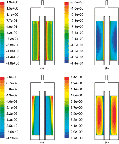
To solve the above system of governing equations, the appropriate boundary and initial conditions as well as physical properties of all materials have to be prescribed. Properties of the air as well as the liquid and gaseous water were assumed based on the well-known literature 23,24. For the dry paper only very little data is available in the literature. Moreover paper properties may vary depending on its internal structure. Values of the specific heat capacity, the heat conduction coefficient and density were prescribed to be equal to the values for pure cellulose, i.e. the specific heat capacity is 1340 J kg⁻¹ K⁻¹), the heat conduction coefficient is 0.335 W m⁻¹ K⁻¹ and the density is 1550 kg m⁻³ 25. As already mentioned, the value of the lumped diffusion coefficient of water in the analysed paper was measured experimentally and a value equal to 10⁻⁹ m² s⁻¹ was obtained. Nevertheless, all the above values together with the evaporation constant (but except the density) were considered to be uncertain and undergone sensitivity analysis. In Figure 1, the values of the relative sensitivity coefficients of the temperature field inside the paper with respect to the heat conduction coefficient (a), the evaporation constant (b), the lumped diffusion coefficient of water in paper (c) and the specific heat capacity (d) are shown. Relative sensitivity coefficients Z_r,P (dimensionless) of the temperature T with respect to the parameter P is defined as (13) At the same time, to increase the credibility of the featured mathematical model of the vacuum drying process, a special experiment was carried out. During this experiment temperatures have been recorded and then used in an inverse analysis. The evaporation constant C_mt in Hertz–Knudsen equation (9) and the initial moisture concentration within the bushing X(x, 0) at the beginning of the vacuum period of the process were selected for the inverse analysis. The sensitivity analysis results showed that the model is very sensitive to the value of the evaporation constant, see Figure 1. Fairly high values of the sensitivity coefficients were obtained also for the specific heat capacity of the dry paper. Nevertheless, the initial moisture field and the evaporation constant were considered as significantly more uncertain in the whole model than all other parameters.

Figure 1. Relative sensitivity coefficients of temperature field after 100 s after beginning of the vacuum period with respect to heat conduction coefficient (a), evaporation constant (b), lumped diffusion coefficient of water in paper (c) and specific heat capacity (d).

3. Experiments and inverse analysis

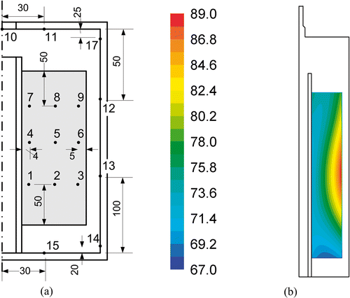
The most important element of the special experimental stand was a vacuum chamber with bushing (paper coil), as shown in Figure 2. The stand allows one to carry out one heating-vacuum cycle of the process. The heating period lasts about 6 h after which the vacuum is applied for about half an hour. Temperatures are recorded at the walls of the vacuum chamber as well as inside the paper coil (representing bushing) by the set of thermocouples. The location of thermocouples within half of the coil vertical cross-section is shown in cf. Figure 3(a). The measurements collected by thermocouples 1–9 are divided into two sets: ‘teaching data’ and ‘testing data’. It is obvious that the longer the sampling time for ‘teaching data’, the more accurate calculations are. On the other hand, the long sampling time lengthens the computation time. Therefore the length of sampling time needs to be a compromise between accuracy and CPU time. In this work 50 s of measurements to collect ‘teaching data’ are chosen.

Figure 2. Parts of the paper vacuum drying experimental stand: (a) vacuum chamber and (b) paper coil with thermocouples.

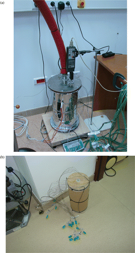
Figure 3. Thermocouples arrangement within (a) the paper coil and (b) initial temperature field. Dimensions are in millimetres and temperatures are in degrees Celsius.

As already mentioned the aim of the inverse analysis is to retrieve the value of selected quantities – the evaporation constant and the moisture distribution within the paper coil at the beginning of the sucking out stage of the process utilizing temperature measurements at nine points located inside the paper coil, cf. Figure 3(a). The objective function typically consists 26,27 of a sum of squares of deviation between temperature measured during the experiment and that predicted by the mathematical model discussed in Section 2, i.e. (14) where T(P) and T * are the vectors of predicted and measured temperatures, respectively. The vector P contains the unknown model parameters which are to be computed through the inverse procedure. It consists of the evaporation constant C_mt (see Equation (9)) and either approximation coefficients of the initial moisture distribution field or initial moisture content in the collocation points (temperature measurement points), cf. Section 3.2. Since all sensors used for temperature measurements are of the same type, the covariance matrix 26 is omitted in Equation (14).

The complexity of the featured inverse problem arises from the fact that model parameters and initial condition are being estimated simultaneously. To solve this problem the Levenberg–Marquardt (L–M) method 27,28 is used to update in an iterative procedure unknown parameters values collected in vector P^k+1 (15) where Z(P) is the sensitivity matrix calculated here by central final differences, e.g. 26,27. Parameter λ is the damping parameter while E is the diagonal matrix. To some extend it is arbitrary how E matrix is determined but most commonly it is just a main diagonal of the matrix Z^T(P^k)Z(P^k) (16)

Although the L–M method is well-known to be very efficient for solving the least square problems, its performance significantly depends on the initial guess. In an analyzed problem, this initial guess is even more important than usual, because to reduce the CPU time, the sensitivity matrix for the L–M algorithm will be determined only once (just for guess solution). Thus, due to the fact that the resulting algorithm may fail to converge, the initial guess cannot be completely arbitrary. Proper determination of the initial guess requires approximation of the initial temperature field as well as the initial moisture distribution within the paper coil.

3.1. Approximation of the initial temperature field

The initial temperature field T₀(x) at an arbitrary spatial point x was approximated with a linear combination of nine (equal to the number of measuring points in the paper coil) two-dimensional multiquadrics radial basis functions (MQ RBFs): (17) where α_i is the approximation coefficient, xⁱ is the RBFs collocation vector and φ(‖x − xⁱ‖) is the i-th MQ RBF. RBFs are commonly used approximation functions whose arguments are distances from function base point, defined as an Euclidean norm. MQ RBF 29 is defined as (18) where x_j is the j-th component of the position vector x, is the j-th component of the i-th RBFs collocation point and c is the function shape parameter. Coefficients of the approximation function (17) were found as a solution of the following set of equations (19) The first nine equations reflect the condition that the estimated temperature (17) at the measurement points must be equal to the measured value. The following equations impose the constraint that temperature derivatives within the aluminium rod with respect to vertical coordinate are negligible, due to very high thermal conductivity of that material. These equations add extra five collocation points located along the aluminium rod (not shown in Figure 3a).

The set of equations (19) is certainly overdetermined – it contains 14 equations and only nine unknown coefficients. Its least square solution produced the resulting temperature field which is shown in Figure 3(b).

3.2. Approximation of the initial moisture distribution

When approximating the initial moisture distribution it was assumed that the moisture diffusion within the paper is negligible and thermodynamic equilibrium between humid air and moisture within the paper at the end of heating period was achieved. Utilizing the definition of the sorption isotherms, water content at nine measuring points is determined. Based on these values three approaches to approximate the initial moisture distribution within the paper coil have been proposed and tested.

In the first approach, the initial moisture field was approximated by the linear combination of inverse multiquadrics radial basis functions (IMQ RBFs) φ(‖x − xⁱ‖) (20) The IMQ function reads (21) where c is the function shape parameter. At the collocation point IMQ RBF reaches a value equal to 1 and it decreases towards 0 when the distance from the collocation point is being increased. In this approach, the values of approximation coefficients α_i are sought utilizing the inverse algorithm, as already discussed in Section 3.1. A disadvantage of this approach is the very high sensitivity of the resulting moisture field on the approximation coefficients.

In the second approach, the initial moisture field is also approximated with the linear combination of IMQ RBFs (Equation (20)). However, this time inverse algorithm does not seek the values of the approximation coefficients but rather the values of moisture content at the collocation points.

In the third approach, the two-dimensional second-order polynomial was proposed as the approximation function, i.e. (22) Higher order polynomial cannot be used since there were nine temperature sampling points during the experiment. Six unknown coefficients α₀, … , α₅ are found as a least square solution of nine equations formulated for nine collocation points.

4. Selected results and discussion

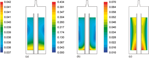
The key results of the inverse analysis are presented in Table 2. The objective function values gathered in this table suggest that the best solution was obtained with the second approach, in which the initial moisture field was approximated with the IMQ RBFs. However, the initial moisture distribution must fulfill the constrain that the total moisture content at the beginning of the sucking out stage has to be lower than its value before experiment. Total moisture content within the bushing before the experiment was equal to 0.0334 kg. It can be seen that only in both first and third approaches did the approximated initial moisture fields give the lower value of the total moisture content, and this is correct. In the second approach the situation is opposite.

Table 2. Results of the inverse analysis.

Quantity	First approach	Second approach	Third approach
Evaporation	0.5493	0.0391	0.2979
constant, 1 m^−1
α1/X2	6.2858E+00	0.0583	0.0547
α2/X3	5.6129E+00	0.1550	0.1549
α3/X4	−1.1762E+01	0.0848	−0.0758
α4/X5	−1.1433E+01	0.0427	0.0736
α5/X5	−1.0183E+01	0.1220	−0.0623
α6/X6	2.1365E+01	0.0784	0.1062
α7/X7	5.9675E+00	0.0662	−0.0449
α8/X8	5.3273E+00	0.1048	0.0621
α9/X9	−1.1166E+01	0.0795	0.1037
Initial moisture	0.0193	0.0551	0.0204
content (kg)
Objective	1.399E+03	3.187E+02	3.755E+02
function value

Since all the three tested approaches produced different values of the initial moisture content, the remaining values presented in Table 2 should not be compared directly. They should rather be perceived through the moisture field that they produce. Based on the above data the initial moisture distribution obtained with the first, the second and the third approximation approach is shown in Figure 4.

Figure 4. Initial moisture distribution obtained with: (a) the first approximation approach, (b) the second approximation approach and (c) the third approximation approach.

Closer examination of the temperature records at the sampling points (where thermocouples were placed) shows that although objective function is the lowest one in the second approach, better behaviour is revealed in the third approach. Firstly, the condition imposed on the total moisture content is fulfilled, secondly, results obtained with this approach predict better temperature readings for a process time that is greater than 50 s. The second approach gives a very good fitting in the time interval which underwent inverse analysis and it fails for times higher than 50 s. A possible reason is the overestimated value of the evaporation constant obtained from the inverse analysis. It should also be mentioned that this approach is characterized by the best conditioning.

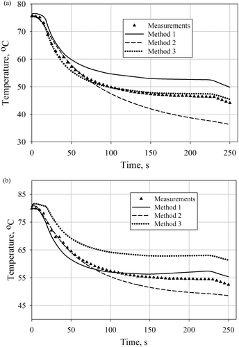
Exemplary comparison of temperature histories obtained for the first, second and the third approximation approach with the measurements is shown in Figure 5.

Figure 5. Comparison of temperature histories obtained for the first, the second and the third approximation approach with the measurements at points no 2: (a) the best fitting and 3 (b) the worst fitting.

5. Conclusions

Although all inverse problems are thought to be ill-posed, estimation of the unknown/uncertain model parameters and/or some fields through inverse analysis was successfully applied to compute evaporation constant and moisture field at the beginning of the sucking out period of experiment. From all the three developed approaches the best results were obtained with the third one. It satisfied the condition imposed on the total moisture content within the bushing and predicted satisfactorily course of the process after 50 s measurements used by the inverse analysis. The second approach gave a fairly good matching of the model to the experimental results but only within a time period which underwent inverse analysis. Results for times higher than 50 s, significantly diverged from the experimental results. The first approach definitely performed worse, being at the same time strongly ill-conditioned. Hence, it cannot be recommended.

To conclude, the second approach and third approach are both promising for further development, although they both need some improvement. First of all, the first-order regularization technique seems to be appropriate for determination of the evaporation constant. Although the value of this constant is not exactly known, analyses carried out brought some information on its order. Utilization of this information should limit possibilities of diverging off this value, as happened in the case of the second approach. Second, sampling (i.e. collocation) points should be positioned closer to the external surface of the bushing domain. Finally, experimental information on the total amount of water at the beginning of the sucking out period could considerably help to stabilize the inverse problem solution.

References

- Getson, DM, 2002. High Voltage Bushings. Germany: ABB Materials; 2002.
- Russek, RM, 1967. Drying and impregnation of paper-insulated power cables, IEEE Trans. Power Apparatus Syst. PAS-86(1) (1967), pp. 34–52.
- Kowalski, SJ, 2003. Thermomechanics of Drying Processes, . Berlin, Heidelberg: Springer-Verlag; 2003.
- Strumiłło, Cz, 1975. Fundamentals of Drying Theory. Warsaw: WNT; 1975, (in Polish).
- Coumans, WJ, 2000. Models for drying kinetics based on drying curves of slabs, Chem. Eng. Process. 39 (2000), pp. 53–68.
- Kroes, B, 1999. "Influence of material properties on drying kinetics". In: Ph.D. Thesis. Eindhoven: Technical University of Eindhoven; 1999.
- Bear, J, and Bachmat, Y, 1990. Introduction to Modeling of Transport Phenomena in Porous Media. Dordrecht: Kluwer Academic; 1990.
- Nield, DA, and Bejan, A, 1999. Convection in Porous Media. New York: Springer-Verlag; 1999.
- Coumans, WJ, and Kruf, WMA, 1995. Mechanistic and lump approach of internal transport phenomena during drying of paper sheet, Drying Technol. 13 (4) (1995), pp. 985–998.
- Cheng, X, and Fan, J, 2004. Simulation of heat and moisture transfer with phase change and mobile condensates in fibrous insulation, Int. J. Thermal Sci. 43 (2004), pp. 665–676.
- Singhal, AK, Athavale, MM, Li, H, and Jiang, Y, 2002. Mathematical basis and validation of the full cavitation model, J. Fluids Eng. 124 (2002), pp. 617–624.
- Karlsson, M, and Stenström, S, 2005. Static and dynamic modeling of cardboard drying, Part 1: Theoretical model, Drying Technol. 23 (2005), pp. 143–163.
- Nowak, AJ, Buliński, ZP, Kasza, K, and Matysiak, Ł, 2008. "Thermodynamic Analysis of the Paper Vacuum Drying Process and the Experimental Validation of Its Computational Model". In: Proceedings of the XX Jubileuszowy Zjazd Termodynamików. Wrocław, Poland: Tom II; 2008. pp. 115–121.
- Nowak, AJ, Buliński, Z, Kasza, K, and Matysiak, Ł, Experimntal Analysis of Vacuum Drying of the High Voltage Bushing. Presented at Proceedings of the World Conference on Experimental Heat Transfer, Fluid Flow and Thermodynamics, ExHFT-7. Cracow, Poland, 2009, (invited paper).
- Nowak, AJ, Buliński, Z, and Kasza, K, , Ł Matysiak, Computational model and experimental validation of the paper vacuum drying process, Int. J. Heat Mass Transfer (submitted for publication).
- FLUENT 6.3 User's Guide, Fluent.Inc, Lebanon, USA, 2006.
- FLUENT 6.3 User Defined Function Manual, Fluent.Inc, Lebanon, USA, 2006.
- Buliński, ZP, Nowak, AJ, Kasza, K, and Matysiak, Ł, 2008. "Initial Inverse Problem in the Vacuum Paper Drying Process". In: Proceedings of the 8th World Congress on Computational Mechanics (WCCM8) and 5th European Congress on Computational Methods in Applied Sciences and Engineering (ECCOMAS 2008). Venice, Italy. 2008.
- Chemkhi, S, and Zagroubba, F, 2005. Water diffusion coefficient in clay material from drying data, Dessalination 185 (2005), pp. 491–498.
- Hamdami, N, Monteau, JY, and Le Bail, A, 2004. Transport properties of a high porosity model food at above and sub-freezing temperatures: Part 2. Evaluation of the effective moisture diffusivity from drying data, J. Food Engin. 62 (2004), pp. 385–392.
- Ergun, S, and Orning, AA, 1952. "Fluid Flow Through Packed Columns". In: Chemical Engineering Progress. Vol. 48. New York: American Institute of Chemical Engineers; 1952. pp. 89–94.
- Clayton, CT, 2006. Multiphase Flow Handbook. Boca Raton, FL: CRC Press Taylor & Francis; 2006.
- Lemmon, EW, Jacobsen, RT, Penoncello, SG, and Friend, D, 2000. Thermodynamic properties of air and mixtures of nitrogen, argon, and oxygen from 60 to 2000 K at pressures to 2000 MPa, J. Phys. Chem. Ref. Data 29 (2000), pp. 331–386.
- Kestin, J, Sengers, JV, Kangmar-Parsi, B, and Levelt Sengers, JMH, 1984. Thermophysical Properties of Fluid H2O, J. Phys. Chem. Ref. Data 13 (1984), pp. 175–183.
- Nilson, J, and Stenetröm, S, 2001. Modelling of heat transfer in hot pressing and impulse drying of paper, Drying Technol. 19 (10) (2001), pp. 2469–2485.
- Kurpisz, K, and Nowak, AJ, 1995. "Inverse Thermal Problems". In: International Series on Computational Engineering. Southampton: Computational Mechanics Publications; 1995.
- Özisik, MN, and Orlande, HRB, 2000. Inverse Heat Transfer: Fundamentals and Application, . New York: Taylor & Francis; 2000.
- Press, WH, Flannery, BF, Teukolsky, SA, and Wetterling, WT, 1989. Numerical Recipes, . New York: Cambridge University Press; 1989.
- Kansa, EJ, and Hon, YC, 2000. Circumventing the ill-conditioning problem with multiquadrics radial basis functions: Applications to elliptic partial differential equations, Comput. Math. Appl. 39 (7–8) (2000), pp. 123–137.