Identification of materials in a hyperbolic annular fin for a given temperature requirement

Abstract

This article deals with the prediction of parameters in an annular hyperbolic fin with temperature-dependent thermal conductivity. Three parameters such as thermal conductivity, variable conductivity coefficient and the surface heat transfer coefficient have been predicted for satisfying a prescribed temperature distribution on the surface of fin. This is achieved by a hybrid differential evolution-nonlinear programming optimization method. The effect of random measurement errors is also considered. It is observed from the present inverse analysis that many feasible materials exist satisfying the given temperature distribution, thereby providing engineering flexibility in selecting any material from the available choices. For a given material, this is possible by regulating the surface heat transfer coefficient.

Keywords:

• inverse prediction
• hyperbolic annular fin
• material identification
• variable conductivity
• hybrid method

Introduction

The analysis of fins is one of the important fields of research in the area of energy and heat transfer.[1,2] The temperature distribution in a fin invariably depends on several factors such as boundary conditions, thermo-physical parameters such as thermal conductivity, dimensions and heat transfer coefficient. Considerable amount of studies can be found in the available literatures mainly addressing the methodology of calculating the steady-state temperature distributions from the knowledge of thermo-physical properties and boundary conditions.[3–8] One of the ways of obtaining the temperature profile is to conduct an experiment by maintaining proper conditions. However, it is well known that for saving the time, money and manpower, a computational study is preferable. In order to computationally obtain the result, the heat transfer equation needs to be solved by a suitable method using known thermo-physical properties and boundary conditions. But, the solution of the governing equation may not be always easy due to difficulties such as nonlinearities and singularities. Due to this, many analytical and numerical methods have been developed for evaluating the performance of different fins. The procedure of computing the desired performance parameter such as temperature distribution is known as well-posed forward method.[9,10] However, the situation becomes complex and more interesting when the objective is to search for unknown thermo-physical parameters which can satisfy a particular temperature field. Such cases fall under the purview of inverse prediction problems [11–13] and their solution is not necessarily unique. In other words, several possible combinations of unknowns satisfying a given requirement may exist,[14] and thus, the inverse problems are relevant for designing an engineering system [15] and are pertinent to industrial processes.[16]

It is observed that for fins, the study of inverse problems is relatively new. Nevertheless, details of few significant inverse problems in fins can be found in literature. For example, using a least squares method (LSM), the estimation of the heat flux at the base of a pin fin was done by Chang et al. [17]. Huang and Hsiao [18] used the conjugate gradient method (CGM) for estimating the shape of spine and longitudinal fins. Using CGM, Lee et al. [19] estimated the heat flux in pin fins. Chen and Hsu [20] used LSM for estimating the heat transfer coefficient in annular finned-tube heat exchangers. Chen et al. [21] have estimated the convective heat transfer coefficient of an annular fin using CGM, whereas Peng et al. [22] have used the particle swarm algorithm for studying plate-fin heat exchangers. Das in [23,24] respectively, used the genetic algorithm (GA) and the simplex search method for inverse heat transfer analyses of cylindrical fin. For rectangular fin geometry, the application of the simulated annealing and the differential evolution (DE) has been done by Das and Ooi [25] and Bhowmik et al. [26], respectively. For a rectangular wet fin, the application of homotopy analysis method along with GA was demonstrated by Panda et al. [27]. For a rectangular moving fin, the decomposition method in conjunction with GA was used by Singla and Das [28]. For inverse problems other than fins, many optimization methods working on different nonlinear programming (NLP) are available in the literature.[29,30]

It is apparent that for solving inverse problems, a suitable optimization algorithm is required for regularisation. The optimization methods are broadly classified as deterministic (gradient-based) and probabilistic (stochastic/evolutionary) possessing separate advantages and disadvantages. For example, gradient-based algorithms are relatively faster [31] but many times get confined to local minima. However, evolutionary algorithms are resistant to local minima but these consume more time.[32] It is observed that compared to other evolutionary optimization algorithms, the DE [33] possesses few advantages such as robustness, fast convergence, compact structure, ease of implementation and its efficacy for optimising nonlinear search domains.[34–37] For combining the benefits of deterministic methods and stochastic methods, recently the usage of hybrid optimization methods is becoming popular.[38]

Based on the above, the focus of the present work is to predict parameters such as the thermal conductivity of the fin material, the coefficient of its variation and the surface heat transfer coefficient for satisfying a prescribed temperature in a hyperbolic annular fin with temperature-dependent thermal conductivity.[39] For optimization, a hybrid DE-NLP algorithm is used due to various advantages of DE and NLP methods as discussed earlier. It is expected that many viable combinations of the unknowns can meet the given desired requirement, which will offer flexibility in selecting any combination among the available alternatives. This in turn enables in identifying potential materials for fabrication of the fin geometry. The following section discusses the formulation and the solution methodology.

Formulation

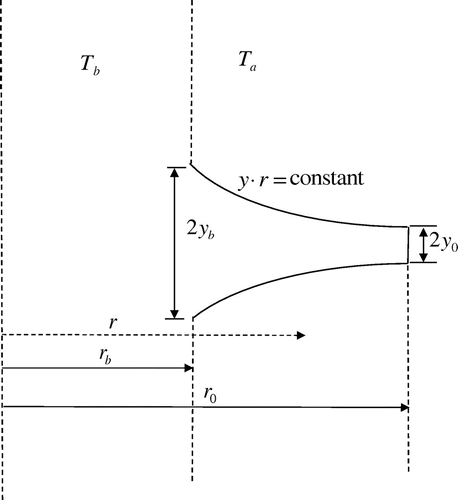
Let us consider a concentric annular fin geometry having hyperbolic profile (obeying y_r = constant) as shown in Figure 1 for which the relevant energy equation is expressed below,[39](1) $$\frac{\text{d}}{\text{d}r}\left(k{A}_{\text{r}}\frac{\text{d}T}{\text{d}r}\right)\text{d}r-A_{\text{s}}h\left(T-T_{\text{a}}\right)=0$$(1)

Figure 1. Geometry of the hyperbolic fin.

where A_r= 2πry_r and A_s= 2πrds are the cross-sectional and lateral surface areas, respectively. For solving Equation (1(1) $$\frac{\text{d}}{\text{d}r}\left(k{A}_{\text{r}}\frac{\text{d}T}{\text{d}r}\right)\text{d}r-A_{\text{s}}h\left(T-T_{\text{a}}\right)=0$$(1) ), the relevant boundary conditions are mentioned below,(2) $$\begin{array}{c}T=T_{\text{b}};r=r_{\text{b}}\hfill \\ \frac{\text{d}T}{\text{d}r}=0;r=r_0\hfill \end{array}$$(2)

In Equation (1(1) $$\frac{\text{d}}{\text{d}r}\left(k{A}_{\text{r}}\frac{\text{d}T}{\text{d}r}\right)\text{d}r-A_{\text{s}}h\left(T-T_{\text{a}}\right)=0$$(1) ), the thermal conductivity is considered to be linearly dependent upon the temperature as mentioned below,(3) $$k=k_{\text{a}}\left\{1+\mathit{\beta }\left(T-T_{\text{a}}\right)\right\}$$(3)

where β is the coefficient of variable thermal conductivity which may be either positive, negative or even zero. Next, assuming the elemental lengths to be equal (i.e. ds = dr), Equation (1(1) $$\frac{\text{d}}{\text{d}r}\left(k{A}_{\text{r}}\frac{\text{d}T}{\text{d}r}\right)\text{d}r-A_{\text{s}}h\left(T-T_{\text{a}}\right)=0$$(1) ) can be alternatively represented in the following manner,[39](4) $$\frac{\text{d}}{\text{d}r}\left(kr{y}_{\text{r}}\frac{\text{d}T}{\text{d}r}\right)-rh\left(T-T_{\text{a}}\right)=0$$(4)

Next, the non-dimensionalization is carried out using the following parameters,(5) $$\mathit{\theta }=\frac{T-T_{\text{a}}}{T_{\text{ref}}-T_{\text{a}}};m=r_0\sqrt{\frac{h}{k_{\text{a}}{y}_{\text{b}}}};r^{*}=\frac{r}{r_0};\mathit{\epsilon }=\mathit{\beta }\left[T_{\text{ref}}-T_{\text{a}}\right]$$(5)

In the forward problem, T_ref =T_b. After non-dimensionalization, Equation (4(4) $$\frac{\text{d}}{\text{d}r}\left(kr{y}_{\text{r}}\frac{\text{d}T}{\text{d}r}\right)-rh\left(T-T_{\text{a}}\right)=0$$(4) ) takes the following form,[39](6) $$\left(1+\mathit{\epsilon }\mathit{\theta }\right)\frac{{\text{d}}^2\mathit{\theta }}{\text{d}{r}^{*2}}+\mathit{\epsilon }{\left(\frac{\text{d}\mathit{\theta }}{\text{d}{r}^{*}}\right)}^2-\frac{r^{*}}{r_{\text{b}}^{*}}{m}^2\mathit{\theta }=0$$(6)

Consequently, the boundary conditions also modify in the following manner,(7) $$\begin{array}{c}\mathit{\theta }=1;r^{*}=r_{\text{b}}^{*}\hfill \\ \frac{\text{d}\mathit{\theta }}{\text{d}{r}^{*}}=0;r^{*}=1\hfill \end{array}$$(7)

The governing equation (Equation (7(7) $$\begin{array}{c}\mathit{\theta }=1;r^{*}=r_{\text{b}}^{*}\hfill \\ \frac{\text{d}\mathit{\theta }}{\text{d}{r}^{*}}=0;r^{*}=1\hfill \end{array}$$(7) )) is a second-order nonlinear ordinary differential equation (ODE) and it can be represented in terms of two first-order ODEs in another variable, η as below,(8) $$\begin{array}{c}\frac{\text{d}\mathit{\theta }}{\text{d}{r}^{*}}=\mathit{\eta }=\mathit{\theta }\left(2\right)\hfill \\ \frac{{\text{d}}^2\mathit{\theta }}{\text{d}{r}^{*2}}=\frac{\text{d}\mathit{\eta }}{\text{d}{r}^{*}}=\frac{1}{\left[1+\mathit{\epsilon }\mathit{\theta }\left(1\right)\right]}\left[\frac{r^{*}}{r_{\text{b}}^{*}}{m}^2\mathit{\theta }\left(1\right)-\mathit{\epsilon }\mathit{\theta }{\left(2\right)}^2\right]\hfill \end{array}$$(8)

where $\mathit{\theta }\left(1\right)$and $\mathit{\theta }\left(2\right)$ are two variables which using some initial guess are updated until the boundary conditions are satisfied. This is done when the residual error, ξ representing boundary conditions is minimised in the following manner,(9) $$\mathit{\xi }=max.\left|\mathit{\theta }{\left(1\right)}_{\left(r^{*}=r_{\text{b}}^{*}\right)}-1;\mathit{\theta }{\left(2\right)}_{\left(r^{*}=1\right)}\right|<{\text{10}}^{\text{- 6}}$$(9)

For known values of non-dimensional parameters (such as m, ε and $r_{\text{b}}^{*}$) which implicitly depend upon dimensional entities (such as k_a, r₀, r_b, y_b and T_a), in the present work, the local non-dimensional temperature (i.e. θ vs. r^*) is obtained by solving the governing equation using bvp4c function available in Matlab which applies an implicit fourth-order Runge–Kutta (RK-4) method involving Lobatto IIIa scheme. The collocation formula provides a C¹-continuous solution in which the mesh selection and error control are based upon the residual of the continuous solution. For solving different problems in science and engineering, details about the bvp4c algorithm can be found elsewhere.[40–44]

Next, considering a situation where some temperature distribution, θ is available from a reliable source. However, three parameters (h, k_a and β) are unknown and the objective is to estimate the three unknowns which shall satisfy the given local temperature distribution, θ. For a given dimension and ambient along with boundary conditions, the estimation of thermal conductivity, k_a, and coefficient of its variation, β, directly give insights about the feasible fin material, whereas the knowledge of surface heat transfer coefficient, h, enables to maintain the appropriate rate of airflow over it. For this task, an inverse problem is solved by minimising the following objective function,(10a) $$F={\left({\mathit{\theta }}_{j=1}-{\tilde{\mathit{\theta }}}_{j=1}\right)}^2+{\left({\mathit{\theta }}_{j=\left(N+1\right)/2}-{\tilde{\mathit{\theta }}}_{j=\left(N+1\right)/2}\right)}^2+{\left({\mathit{\theta }}_{j=N}-{\tilde{\mathit{\theta }}}_{j=N}\right)}^2$$(10a) (10b) $$\text{Since},{\mathit{\theta }}_{j=1}={\tilde{\mathit{\theta }}}_{j=1}=1.0,\text{so},F={\left({\mathit{\theta }}_{j=\left(N+1\right)/2}-{\tilde{\mathit{\theta }}}_{j=\left(N+1\right)/2}\right)}^2+{\left({\mathit{\theta }}_{j=N}-{\tilde{\mathit{\theta }}}_{j=N}\right)}^2$$(10b)

where N is the number of divisions in which the entire radial domain of the fin is divided to ensure satisfactory generation of the temperature distribution, θ and for the present work, N = 61 is considered. It is worth to mention here that Equations (1(1) $$\frac{\text{d}}{\text{d}r}\left(k{A}_{\text{r}}\frac{\text{d}T}{\text{d}r}\right)\text{d}r-A_{\text{s}}h\left(T-T_{\text{a}}\right)=0$$(1) )–(7(7) $$\begin{array}{c}\mathit{\theta }=1;r^{*}=r_{\text{b}}^{*}\hfill \\ \frac{\text{d}\mathit{\theta }}{\text{d}{r}^{*}}=0;r^{*}=1\hfill \end{array}$$(7) ) are connected to each other, and for solving the inverse problem, the entire step (from Equations (1(1) $$\frac{\text{d}}{\text{d}r}\left(k{A}_{\text{r}}\frac{\text{d}T}{\text{d}r}\right)\text{d}r-A_{\text{s}}h\left(T-T_{\text{a}}\right)=0$$(1) ) to (7(7) $$\begin{array}{c}\mathit{\theta }=1;r^{*}=r_{\text{b}}^{*}\hfill \\ \frac{\text{d}\mathit{\theta }}{\text{d}{r}^{*}}=0;r^{*}=1\hfill \end{array}$$(7) )) is processed. In Equation 10, $\tilde{\mathit{\theta }}$ denotes the known temperature values corresponding to which the unknown parameters are to be estimated and θ represents the temperature distribution calculated using some arbitrary guessed values of the unknowns, which are updated iteratively. In the inverse problem, the temperature distribution, $\tilde{\mathit{\theta }}$ is assumed to be available at three locations, two at the boundaries (${\tilde{\mathit{\theta }}}_1,{\tilde{\mathit{\theta }}}_{\text{N}}$) and the other one at the centre (${\tilde{\mathit{\theta }}}_{\left(N+1\right)/2}$). The exact temperature distribution of Equation (10) (i.e. $\tilde{\mathit{\theta }}$) may be affected by noise (random errors, e_r). In the present work, additive white Gaussian random measurement error, e_r is considered. In order to consider this effect, the objective function, F modifies as below,(11a) $$F={\left[{\mathit{\theta }}_{j=1}-\left({\tilde{\mathit{\theta }}}_{j=1}+e_r\right)\right]}^{\text{2}}+{\left[{\mathit{\theta }}_{j=\left(N+1\right)/2}-\left({\tilde{\mathit{\theta }}}_{j=\left(N+1\right)/2}+e_r\right)\right]}^2+{\left[{\mathit{\theta }}_{j=N}-\left({\tilde{\mathit{\theta }}}_{j=N}+e_{\text{r}}\right)\right]}^2$$(11a) (11b) $$\text{Since}{\mathit{\theta }}_{j=1}={\tilde{\mathit{\theta }}}_{j=1}=1.0,\text{so},F=e_{\text{r}}^2+{\left({\mathit{\theta }}_{j=\left(N+1\right)/2}-{\tilde{\mathit{\theta }}}_{j=\left(N+1\right)/2}-e_{\text{r}}\right)}^2+{\left({\mathit{\theta }}_{j=N}-{\tilde{\mathit{\theta }}}_{j=N}-e_{\text{r}}\right)}^2$$(11b)

The practical relevance of Equations (10) and (11) is discussed below.

In the present work, the reference temperature (exact base temperature) is assumed to (T_ref = 460 K) in both forward and inverse models. But, the measurement of base temperature in actual practice is susceptible to measurement errors. So, only when the base temperature is correctly measured, in that case only the non-dimensional temperature $\left(\text{i.e}.{\mathit{\theta }}_{j=1}=\frac{T\left(=T_{\text{b}}\right)-T_{\text{a}}}{T_{\text{ref}}\left(=T_{\text{b}}\right)-T_{\text{a}}}\right)$ will be 1.0. So, in the inverse problem, only T_ref =460 K is assumed to be known and is kept unaltered. The only available information about the base is that it is maintained at a uniform temperature (therefore, ${\tilde{\mathit{\theta }}}_{j=1}=1$) and the objective is to search for feasible dimensional parameters related to the fin material (h, k_a and β). In other words, due to uncertainties/measurement errors, even with the same instrument, an exact temperature of 460 K may be interpreted on different occasions as 460.01, 459.91, 460.05, etc. and it is not certain what is the actual (correct) value of the base temperature. Therefore, the reference temperature in that case may be evaluated by taking sufficiently large number of temperature data and computing their mean. Similar issue happens when measuring the ambient temperature, T_a. Therefore, the measurement error (e_r) takes care of all such uncertainties. Due to this, θ at the base (inner radius) will not be equal to 1.0 in such case (and will be ${\tilde{\mathit{\theta }}}_{j=1}+e_{\text{r}}$ = 1 + e_r). But, in the inverse solver, the boundary condition happens to be just θ_j=1= 1 (as the inverse solver solves/regularises the non-dimensional form of the equations and various dimensional parameters being embedded within the non-dimensional form).

For a prescribed range (±e_r), it may be worthy to mention here that the measurement errors being random in nature, their absolute magnitudes at the three locations ($1,(N+1)/2$ and N) as considered in the above objective function (Equation (11)) may not correspond to the maximum value. So, the objective function involving measurement error may be modified in the following manner,(12) $$F={\left[{\mathit{\theta }}_{j\to e_{\text{r}}\left(max.\right)}-\left({\tilde{\mathit{\theta }}}_{j\to e_{\text{r}}\left(max.\right)}+e_{\text{r}}\right)\right]}^{\text{2}}+{\left[{\mathit{\theta }}_{j\to e_{\text{r}}\left(min.\right)}-\left({\tilde{\mathit{\theta }}}_{j\to e_{\text{r}}\left(min.\right)}+e_{\text{r}}\right)\right]}^2+{\left[{\mathit{\theta }}_{j=N}-\left({\tilde{\mathit{\theta }}}_{j=N}+e_{\text{r}}\right)\right]}^2$$(12)

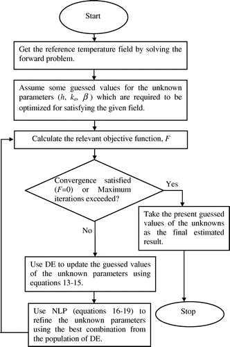
where $e_{\text{r}}\left(max.\right)$ and $e_{\text{r}}\left(min.\right)$, respectively, represent the locations of maximum and minimum limits of the measurement errors, e_r. The flowchart representing the solution methodology of the inverse problem is shown in Figure 2. Now, for estimating the unknown parameters (h, k_a and β), the minimization of the objective function, F, is carried out by an optimization algorithm, which is discussed below.

Figure 2. Flowchart of the inverse method.

Optimization algorithm

As discussed previously that the deterministic and the evolutionary methods have diverse merits and demerits. Therefore, it is good to combine the two methods and form a hybrid algorithm which can perform better than any of the two individual algorithms. In this work, DE is used to perform an exhaustive searching and then the best solution of a particular iteration is made to act as an initial guess for NLP, thus further refining the solution. In DE, a fixed number of random possible solutions (known as the population) are generated, which is considered to be 25 for this work. If the termination condition is unsatisfied, then the population is updated in an iterative manner using operators such as crossover and mutation. The termination condition is assumed either when the objective function, F becomes zero or the hybrid algorithm exceeds 11 iterations, which is found to be reasonably sufficient. The population is generated between the upper and lower bounds of the unknowns consisting of vectors of size n, where n is the number of unknown parameters (three, in the present work). Then, for a given vector, Z_k (k denotes the index of iteration level), five distinct vectors $\left[\left(a,b,c,d,e\right)\ne Z_{\text{k}}\right]$ each consisting of n members are randomly selected. Next, a mutant for the parent vector, Z_k is generated using the following scheme,(13) $$Y_{\text{k}}=a_{\text{k}}+\mathit{\omega }\frac{\left(b_{\text{k}}-c_{\text{k}}\right)+\left(d_{\text{k}}-e_{\text{k}}\right)}{2}$$(13)

where ω is the scaling factor and for the present work, its value is considered to be 0.7. After this, the child vector, z_k is selected between the parent and mutant vectors (i.e. Z_k and Y_k) using the following criteria,(14) $$\begin{array}{c}{z}_{\text{k}}=Z_{\text{k}};\Re >\mathit{\chi }\hfill \\ z_{\text{k}}=Y_{\text{k}};\Re \le \mathit{\chi }\hfill \end{array}$$(14)

where $\Re \in \left[0,1\right]$ is a random number and χ is the crossover probability, which is considered to be 0.9 for this study.[26] It is to be noted that all vectors (a, b, c, d, e, Z, z, Y) involve discrete values of unknown parameters (k_a, β, h). The final retention of either the child, z_k, or the parent, Z_k, is based upon the following condition,(15) $$\begin{array}{c}\text{if},F\left(z_{\text{k}}\right)\le F\left(Z_{\text{k}}\right);\text{then},z_{\text{k}}=Z_{\text{k}}\hfill \\ \text{else},(\text{i.e.}F\left(Z_{\text{k}}\right)>F\left(z_{\text{k}}\right));Z_{\text{k}}=z_{\text{k}}\hfill \end{array}$$(15)

The above-mentioned constitutes one iteration of DE. As mentioned earlier, the best solution of DE is subjected to NLP algorithm. NLP is an efficient local search method which is relatively faster due to usage of both first- and second-order derivatives. There occurs a lowest and highest searching limit for each parameter$\left(\text{i}\text{.e}\text{.}{k}_{\text{a}},\mathit{\beta },h\right).$ Therefore, the following serves as constraints,(16) $$j_{\text{i}}\left(n\right)=\left[\begin{array}{c}h\hfill \\ k_{\text{a}}\hfill \\ \mathit{\beta }+6\times {10}^{-3}\hfill \\ 200-h\hfill \\ 450-k_{\text{a}}\hfill \\ 6\times {10}^{-3}-\mathit{\beta }\hfill \end{array}\right]\ge 0;i=1\dots p$$(16)

In this work, the number of unknowns, n $\in \left(h,k_{\text{a}},\mathit{\beta }\right)$ and constraints, p $\in \left(j_1....j_6\right)$ are equal to three and six, respectively. For a given unknown, n, the Karush–Kuhn–Tucker (KKT) conditions are expressed by the Lagrangian function mentioned below,(17) $$\mathrm{\pounds }\left(n,\mathit{\psi }\right)=F\left(n\right)-\sum _{i=1}^p{\mathit{\psi }}_{\text{i}}{j}_{\text{i}}\left(n\right)$$(17)

where $\mathit{\psi }$ is the Lagrangian multiplier. For present problem, the KKT conditions are evaluated as mentioned below,(18a) $${\mathrm{\nabla }}_{\text{n}}\mathrm{\pounds }\left(n,\mathit{\psi }\right)=0$$(18a) (18b) $${\mathit{\psi }}_{\text{i}}{j}_{\text{i}}\left(n\right)=0;{\forall }_{i=1}^p$$(18b) (18c) $$\begin{array}{c}{j}_{\text{i}}\left(n\right)\ge 0\hfill \\ {\mathit{\psi }}_{\text{i}}\ge 0\hfill \end{array}$$(18c)

For ensuring if a point is either maximum or minimum, the Hessian matrix is obtained as below,(19) $${\mathrm{\nabla }}^2\mathrm{\pounds }\left(n,\mathit{\psi }\right)={\mathrm{\nabla }}^{2}F\left(n\right)-\sum _{i=1}^p{\mathit{\psi }}_{\text{i}}{\mathrm{\nabla }}^2{j}_{\text{i}}\left(n\right)$$(19)

where the two terms on the right hand side represent the Hessian matrices for the objective function and constraints, respectively. In this work, the solution of NLP is obtained by the interior point method which is well-discussed.[45–48] In subsequent section, the results and discussion are provided.

Results and discussion

The prime objective and focus of the present work is to identify feasible materials for a hyperbolic fin using the knowledge of the thermal conductivity at ambient condition, k_a, and coefficient of variable conductivity, β. The approximate estimated values of the thermal conductivity, k_a, and the coefficient of its variation, β, are compared with the usual available values.[49,50] Moreover, the surface heat transfer coefficient h, can also be regulated through appropriate design and manufacturing of the fin system and properly adjusting the airflow over the fin surface, therefore, it is also estimated through the inverse analysis. The dimension along with ambient and fin base conditions are considered to be fixed as provided in Table 1.

Table 1. Different values of parameters considered to be fixed during the inverse analysis.

Parameters	Values
Reference temperature, Tref	460 K
Base temperature, Tb (only for no measurement error, i.e. er = 0)	460 K
Ambient temperature, Ta	300 K
Tip radius, r0	0.10 m
Base radius, rb	0.025 m
Semi fin thickness, yb	0.0085 m

The exact temperature distribution is obtained using a forward technique involving RK-4 method. For validating the accuracy of the forward method, Figure 3 shows the comparison of local temperature distributions obtained using the forward method with those available in the literature [39] computed using the double decomposition method. For non-dimensional base radius, $r_{\text{b}}^{*}=0.25$ and different values of the non-dimensional fin parameter m, the results have been compared for both positive, negative and zero values of the thermal conductivity parameter, ε. As may be evident, positive values of the thermal conductivity parameter ε, indicate that the thermal conductivity increases with the increase in temperature, where the opposite is true for negative values of the thermal conductivity parameter, ε. It is observed from Figure 3 that both trends are in very good agreement with each other. The results of the inverse problem are discussed below.

Figure 3. Validation of the forward method for different non-dimensional thermo-physical parameters.

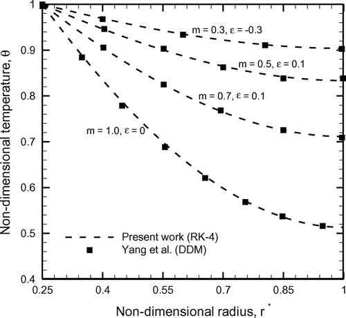
Table 2 presents the estimated values of three unknowns (h, k_a and β) for satisfying a particular temperature distribution considering it to be free of measurement error (i.e. e_r= 0). The CPU time elapsed for executing each run is also illustrated in the table. All executions have been performed using Matlab code on a 32-bit system with Intel Core (TM) i7-3770 CPU with 3.40 GHz clock speed and 2.0 GB RAM. The reference temperature (referred to as exact distribution) corresponding to which the unknowns (h, k_a and β) have been estimated is computed by solving a forward problem using non-dimensional fin parameter, m = 0.7, thermal conductivity parameter, ε = 0.1 and non-dimensional base radius, $r_{\text{b}}^{*}=0.25.$ The estimated values of non-dimensional quantities (ε and m) can be easily obtained from the estimated values of dimensional parameters (h, k_a and β) using the relevant conversion carried out in Equation (5(5) $$\mathit{\theta }=\frac{T-T_{\text{a}}}{T_{\text{ref}}-T_{\text{a}}};m=r_0\sqrt{\frac{h}{k_{\text{a}}{y}_{\text{b}}}};r^{*}=\frac{r}{r_0};\mathit{\epsilon }=\mathit{\beta }\left[T_{\text{ref}}-T_{\text{a}}\right]$$(5) ). In order to estimate the unknowns (h, k_a and β), the objective function mentioned in Equation (10) is minimised using hybrid method. The main outcome of Table 2 is identification of different combination of materials whose thermal conductivity at ambient condition, k_a, and coefficient of variable thermal conductivity, β, approximate to the values as obtained from the inverse analysis. In addition to this, for satisfying the given temperature distribution, the heat transfer coefficient, h, also needs to be adjusted as per the recommended values presented in Table 2. For each run of Table 2, the relevant values of non-dimensional fin parameter, m, and non-dimensional conductivity parameter, ε, are also shown. These non-dimensional parameters (ε and m) can be easily computed using the non-dimensionalization carried out in Equation (5(5) $$\mathit{\theta }=\frac{T-T_{\text{a}}}{T_{\text{ref}}-T_{\text{a}}};m=r_0\sqrt{\frac{h}{k_{\text{a}}{y}_{\text{b}}}};r^{*}=\frac{r}{r_0};\mathit{\epsilon }=\mathit{\beta }\left[T_{\text{ref}}-T_{\text{a}}\right]$$(5) ). It can be seen that the non-dimensional parameters (ε and m) for each case of estimated values of parameters (h, k_a and β) differ from the exact values (m = 0.7 and ε = 0.1). In other words, there exist many feasible combinations of non-dimensional parameters (ε and m) which can result in a similar temperature distribution as obtained with the values m = 0.7 and ε = 0.1. Figure 4 shows the variation of the objective function, F and the estimated unknowns (h, k_a and β) with number of iterations of the hybrid optimization algorithm. The results have been presented only for first case (Run 1) of Table 2. It is observed from Figure 4(a) that the objective function, F gradually minimises and attains a sufficiently low value $O\left(<{10}^{-6}\right)$ in 11 iterations. The objective function, F changes between 1st (initial) and 3rd iterations, then remains constant from 3rd to 6th iteration, decreases again from 6th to 7th iteration, again remains unchanged until 9th iteration, and so on. However, between 3rd and 11 iterations, there is no significant change in the values of the heat transfer coefficient, h, and the thermal conductivity, k_a (Figure 4(b) and (c)). But, during the iterative process, considerable percentage change occurs in the value of coefficient of variable thermal conductivity, β (Figure 4(d)). This clearly indicates that the temperature distribution, θ, is largely dependent upon the value of the variable conductivity coefficient, β, as compared to other two unknowns. After successfully solving the inverse problem and estimating the parameters for a given temperature distribution involving no measurement error, the effect of random measurement error is considered next. For this work, additive white Gaussian measurement error, e_r approximately between ±11% is studied and the relevant details are presented in Figure 5. For this comparison, the exact distribution is the same as obtained earlier using non-dimensional fin parameter, m = 0.7, thermal conductivity parameter, ε = 0.1 and non-dimensional base radius, $r_b^{*}=0.25.$ After incorporation of the measurement error, e_r, the local temperature distribution is also termed as the measured distribution in Figure 5.

Table 2. Estimated values of various unknowns for temperature field without measurement error, e_r = 0. (Forward non-dimensional parameters: m = 0.7, ε = 0.1 and $r_{\text{b}}^{*}$ = 0.25.)

Run	Heat transfer coefficient, h (W[m^2K]^−1)	Thermal conductivity, ka (W [m K]^−1)	Coefficient of variable thermal conductivity, β (K^−1)	Non-dimensional thermal conductivity parameter, ε (estimated)	Non-dimensional fin parameter, m (estimated)	CPU time (s)	Feasible materials[49]
1	24.157	79.365	−1.764 × 10^−3	−0.2822	0.5984	1509	Iron
2	18.740	53.251	−5.870 × 10^−4	−0.0939	0.6434	1511	Carbon steel
3	79.530	204.000	7.211 × 10^−4	0.1154	0.6772	1509	Aluminium
4	6.431	16.545	7.131 × 10^−4	0.1141	0.6762	1512	Stainless steel
5	154.194	400.264	−3.780 × 10^−5	−0.0060	0.6732	1510	Copper

Figure 4. Variation of the objective function, F and unknown parameters (h, k, β) with number of iterations of hybrid algorithm; e_r = 0.

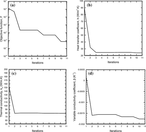
Figure 5. Comparison of the exact and measured temperature fields along with measurement error; m = 0.7, e = 0.1 and $r_{\text{b}}^{*}$ = 0.25.

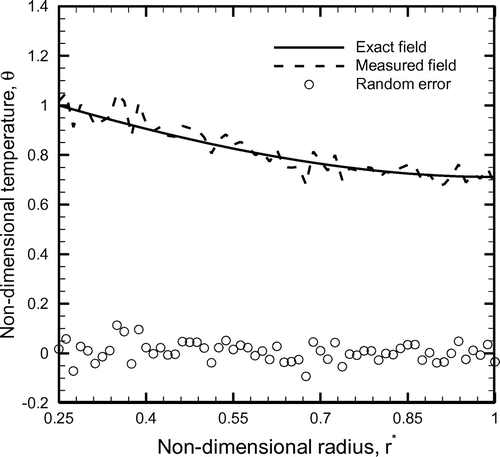
Table 3 presents the estimated values of the three unknowns (h, k_a and β) for yielding a given temperature distribution involving measurement error (i.e. e_r≠ 0). The measured temperature corresponding to which the three unknowns (h, k_a and β) have been estimated is computed by solving a forward problem and by incorporating relevant measurement error, e_r, for non-dimensional parameters indicated in the table. For estimating the three unknowns (h, k_a and β), the objective function, F, as mentioned in Equation (11) is minimised using the hybrid method. In Run 1, two different results have been presented for separate objective functions as detailed earlier in Equations (11) and (12(11a) $$F={\left[{\mathit{\theta }}_{j=1}-\left({\tilde{\mathit{\theta }}}_{j=1}+e_r\right)\right]}^{\text{2}}+{\left[{\mathit{\theta }}_{j=\left(N+1\right)/2}-\left({\tilde{\mathit{\theta }}}_{j=\left(N+1\right)/2}+e_r\right)\right]}^2+{\left[{\mathit{\theta }}_{j=N}-\left({\tilde{\mathit{\theta }}}_{j=N}+e_{\text{r}}\right)\right]}^2$$(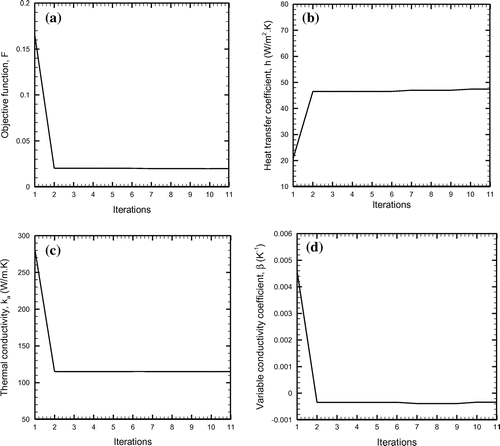11a) ). From results of Table 3, in addition to the relevant values of the heat transfer coefficient, h, many feasible combinations of materials have been identified whose thermal conductivity at ambient condition, k_a, and coefficient of variable thermal conductivity, β, approximate to the values as estimated from the inverse method. Similar observations as made earlier (for the case of no measurement error) are found in this case too. Figure 6 shows the variation of the objective function, F and the estimated unknowns (h, k_a and β) with number of iterations of the hybrid optimization algorithm. The results have been presented only for first case (Run 1a) of Table 3. It is noted from Figure 6(a) that the objective function, F does not change significantly beyond 2nd iteration and its final value is observed to be approximately, $O\left({10}^{-2}\right)$. As such, beyond 2nd iteration, there is no significant update in the values of three estimated parameters (h, k_a and β) as well (Figure 6(b–d)). In this case too, 11 iterations are found to be enough because the objective function, F does not expected to be minimised with further increase in the number of iterations of the hybrid algorithm. Therefore, with incorporation of the measurement error, e_r, the final value of the objective function, F attains relatively higher value as compared to that involving no measurement error. This is due to the reason that when the exact temperature is affected by random noise, the distribution is in the irregular form (Figure 5). However, when the optimization process is executed, the parameters (h, k_a and β) are tuned in such a manner which always result in a smooth reconstructed temperature distribution in the vicinity of the exact distribution as well as ensuring minimum possible deviation between the exact and the reconstructed temperatures. Depending upon the amount of measurement error contained at the three locations (i.e. j = 1, (N + 1)/2 and N), intuitively the objective function is also expected to be minimised up to the equivalent order of measurement error.

Table 3. Estimated values of various unknowns for temperature field with measurement error, e_r≠ 0. (Forward non-dimensional parameters: m = 0.7, e = 0.1 and $r_{\text{b}}^{*}$ = 0.25.)

Run	Heat transfer coefficient, h (W [m^2K]^−1)	Thermal conductivity, ka (W [m K]^−1)	Coefficient of variable thermal conductivity, β (K^−1)	Non-dimensional thermal conductivity parameter, ε (estimated)	Non-dimensional fin parameter, m (estimated)	CPU time (s)	Feasible materials [49,50]
1a (max)	47.419	114.971	−3.356 × 10^−4	−0.0537	0.6966	1510	Zinc
1b (min)	43.991	115.409	−4.207 × 10^−4	−0.0673	0.6697	1509	Zinc
2	27.716	68.401	−6.162 × 10^−4	−0.0986	0.6904	1511	Tin
3	31.537	70.852	1.516 × 10^−4	0.0243	0.7236	1510	Platinum
4	11.681	37.926	−9.000 × 10^−4	−0.1444	0.6020	1508	Alumina
5	20.923	53.748	−5.245 × 10^−4	−0.0839	0.6767	1512	Carbon steel

Figure 6. Variation of the objective function, F and unknown parameters (h, k, β) with number of iterations of hybrid algorithm; e_r≠ 0.

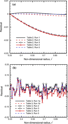
The estimated results of the three unknowns (h, k_a and β) are meaningful only if each set of parameters representing a given material approximates to the exact temperature distribution, which in the present work corresponds to the non-dimensional fin parameter, m = 0.7, thermal conductivity parameter, ε = 0.1 and non-dimensional base radius, $r_{\text{b}}^{*}=0.25.$ The temperature produced by the estimated values of the three unknowns (h, k_a and β) is also known as the reconstructed temperature. Therefore, in Figure 7(a) comparison between the exact and the reconstructed temperature distributions is demonstrated. A very good agreement is observed between the two cases for each of the cases involving no measurement error (Figure 7(a)). However, even with measurement error, Figure 7(b) reveals that the variation in the reconstructed temperature distributions computed using separate objective functions involving different conditions of known temperature locations is very small. For all other cases of materials involving measurement error, the reconstructed and the exact temperature distributions are also found to agree reasonably well with each other as depicted in Figure 7(c). For each run corresponding to Tables 2 and 3, Figure 8 presents a comparison of the residuals (i.e. exact and reconstructed for e_r = 0 and measured and reconstructed for e_r≠ 0). It is quite obvious from the figure that with exact temperature data (i.e. e_r =0), the maximum residual is within 2.0%, whereas for noisy data (i.e. e_r≠ 0), the same being within 15%. Even so, the reconstructed and the exact distributions agree quite satisfactorily as observed earlier in Figure 7.

Figure 7. Comparison of the exact and reconstructed temperature fields, (a) without involving measurement error, e_r = 0, (b) and (c) involving measurement error, e_r≠ 0.

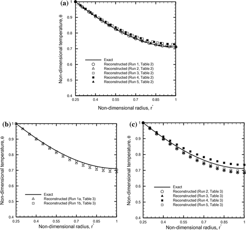
Figure 8. Comparison of the residuals between the exact and the reconstructed temperature fields, (a) without involving measurement error, e_r= 0 and (b) involving measurement error, e_r≠ 0.

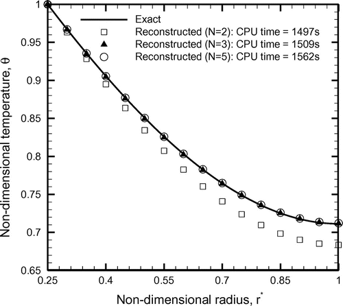
In order to study the effect of number of temperature measurement points, N on the accuracy of the reconstructed temperature, a study is carried out in Figure 9. For a forward problem with m = 0.7, ε = 0.1 and $r_{\text{b}}^{*}$ = 0.25, the results have been presented only for the case involving an exact temperature distribution (i.e. e_r =0). For N = 2, the measurements correspond to θ₁ and θ₃₁, whereas for N = 5, the measurements correspond to θ₁, θ₂₅, θ₃₁, θ₅₀ and θ₆₁. For N = 3, the measurements are assumed to be done at the two boundaries (θ₁ and θ₆₁) and the centre (θ₃₁). Figure 8 reveals that with increase in the number of measurement points, the computational time also increases, whereas the accuracy between the exact and the recovered distribution remains nearly the same. However, with two measurement locations (i.e. N = 2), relatively inferior agreement is observed between the exact and the recovered temperatures. Therefore, for the present problem, minimum three temperature points are required for satisfactory reconstruction of the temperature. The conclusion derived from the present study is discussed next.

Figure 9. Comparison of the exact and the reconstructed temperature fields for different measurement points.

Conclusion

An inverse design of an annular hyperbolic fin with variable thermal conductivity is carried out using hybrid optimization algorithm. For calculating the temperature distribution, a forward numerical scheme involving RK-4 method is used, the results of which are well-validated with those available in the literature. Using temperatures at three discrete locations, three parameters such as the thermal conductivity at ambient condition along with the coefficient of its variation and the surface heat transfer coefficient have been simultaneously estimated using DE-NLP algorithm for attaining a given temperature distribution on the fin surface. The present study provides engineering insights about various feasible materials along with the relevant heat transfer coefficient, thereby affording flexibility in selecting any set of parameters among the available alternatives. Even for the temperature distribution involving measurement errors within a given range, the reconstructed distributions are found to be in reasonably satisfactory agreement with the exact one.

Nomenclature
Ar	=	Cross-sectional area
As	=	Lateral surface area
a, b, c, d, e	=	Vectors in DE algorithm
er	=	Measurement error
F	=	Objective function
h	=	Heat transfer coefficient (W [m2 K]-1)
j	=	Set containing the constraints
k	=	Thermal conductivity (W [m K]-1)
ka	=	Thermal conductivity at ambient condition (W [m K]-1)
m	=	Non-dimensional fin parameter
N	=	Number of temperature measurement points
n	=	Set containing the unknowns
p	=	Number of constraints
r	=	Any location along the radial direction (m)
rb	=	Inner (base) radius of the fin (m)
ro	=	Outer (tip) radius of the fin (m)
r*	=	Non-dimensional radius (=r/r0)
T	=	Temperature (K)
Tb	=	Base temperature (K)
Ta	=	Ambient temperature (K)
Y	=	Mutant vector in DE algorithm
y	=	Semi-thickness of the fin
Z	=	Parent vector in DE algorithm
z	=	Child vector in DE algorithm

Greek symbols
β	=	Variable conductivity coefficient (1/K)
χ	=	Crossover probability in DE algorithm
ε	=	Non-dimensional thermal conductivity parameter
θ	=	(T − Ta)/(Tref – Ta)
$\tilde{\mathit{\theta }}$	=	Exact value of non-dimensional temperature
ω	=	Scaling factor in DE algorithm
ψ	=	Lagrange multiplier in NLP algorithm

References

- Kern QD, Kraus DA. Extended surface heat transfer. New York, NY: McGraw-Hill; 1972.
- Huang CH, Wang DM, Chen HM. Prediction of local thermal contact conductance in plate finned-tube heat exchangers. Inverse Prob. Sci. Eng. 1999;7:119–141.10.1080/174159799088027690
- Kim S, Moon JH, Huang CH. An approximate solution of the nonlinear fin problem with temperature-dependent thermal conductivity and heat transfer coefficient. J. Phys. D: Appl. Phys. 2007;40:4382–4389.10.1088/0022-3727/40/14/038
- Coşkun SB, Atay M. Fin efficiency analysis of convective straight fins with temperature dependent thermal conductivity using variational iteration method. Appl. Therm. Eng. 2008;28:2345–2352.10.1016/j.applthermaleng.2008.01.012
- Khani F, Raji MA, Nejad HH. Analytical solutions and efficiency of the nonlinear fin problem with temperature-dependent thermal conductivity and heat transfer coefficient. Commun. Nonlinear Sci. Numer. Simulat. 2009;14:3327–3338.10.1016/j.cnsns.2009.01.012
- Domairry G, Fazeli M. Homotopy analysis method to determine the fin efficiency of convective straight fins with temperature-dependent thermal conductivity. Commun. Nonlinear Sci. Numer. Simulat. 2009;14:489–499.10.1016/j.cnsns.2007.09.007
- Kundu B. Analytic method for thermal performance and optimization of an absorber plate fin having variable thermal conductivity and overall loss coefficient. Appl. Energy. 2010;87:2243–2255.10.1016/j.apenergy.2010.01.008
- Hajmohammadi MR, Poozesh S, Nourazar SS. Constructal design of multiple heat sources in a square-shaped fin. Proc. Instn. Mech. Eng, E, J. Process Mech. Eng. 2012;226:324–336.10.1177/0954408912447720
- Jaynes ET. The well-posed problem. Found. Phys. 1973;3:477–492.10.1007/BF00709116
- Schweiger M, Arridge SR, Delpy DT. Application of the finite-element method for the forward and inverse models in optical tomography. J. Math. Imaging Vision. 1993;3:263–283.10.1007/BF01248356
- Dobson BJ, Rider E. A review of the indirect calculation of excitation forces from measured structural response data. Proc. Inst. Mech. Eng. C, J. Mech. Eng. Sci. 1990;204:69–75.10.1243/PIME_PROC_1990_204_080_02
- Das R. Estimation of radius ratio in a fin using inverse CFD model. CFD Lett. 2011;3:40–47.
- Fainekos GE, Giannakoglou KC. Inverse design of airfoils based on a novel formulation of the ant colony optimization method. Inverse Probl. Sci. Eng. 2003;11:21–38.10.1080/1068276031000074288
- Das R, Ooi KT. Predicting multiple combination of parameters for designing a porous fin subjected to a given temperature requirement. Energy Convers. Manage. 2013;66:211–219.10.1016/j.enconman.2012.10.019
- Das R, Mallick A, Ooi KT. A fin design employing an inverse approach using simplex search method. Heat Mass Transfer. 2013;49:1029–1038.
- Banim RS, Brett PN, Tierney MJ, Hinds M. Application of inverse methods to temperature measurement in internal mixers. Proc. Inst. Mech. Eng. E, J. Process Mech. Eng. 2003;217:295–306.10.1243/095440803322611660
- Chang MH, Lin JH, Chen CK. The inverse estimation of local heat transfer coefficient in a vertical plate fin with its base subjected to periodically oscillated temperature. Numer. Heat Transfer-A. 2001;40:253–271.10.1080/10407782.2001.10120636
- Huang CH, Hsiao JH. An inverse design problem in determining the optimum shape of spine and longitudinal fins. Numer. Heat Transfer-A. 2003;43:155–177.10.1080/10407780307326
- Lee HL, Chou HM, Yang YC. The function estimation in predicting heat flux of pin fins with variable heat transfer coefficients. Energy Convers. Manage. 2004;45:1749–1758.10.1016/j.enconman.2003.09.017
- Chen HT, Hsu WL. Estimation of heat transfer coefficient on the fin of annular finned-tube heat exchangers in natural convection for various fin spacings. Int. J. Heat Mass Transfer. 2007;50:1750–1761.10.1016/j.ijheatmasstransfer.2006.10.021
- Chen WL, Yang YC, Lee HL. Inverse problem in determining convection heat transfer coefficient of an annular fin. Energy Convers. Manage. 2007;48:1081–1088.10.1016/j.enconman.2006.10.016
- Peng H, Ling X, Wu E. An improved particle swarm algorithm for optimal design of plate-fin heat exchangers. Ind. Eng. Chem. Res. 2010;49:6144–6149.10.1021/ie1002685
- Das R. Application of genetic algorithm for unknown parameter estimations in cylindrical fin. Appl. Soft Comput. 2012;12:3369–3378.10.1016/j.asoc.2012.07.005
- Das R. Three-parameter estimation study in a radial fin geometry using FDM-based simplex method. Heat Transfer Eng. 2014;35:1309–1319.10.1080/01457632.2013.876866
- Das R, Ooi KT. Application of simulated annealing in a rectangular fin with variable heat transfer coefficient. Inverse Prob. Sci. Eng. 2013;21:1352–1367.10.1080/17415977.2013.764294
- Bhowmik A, Singla RK, Roy PK, Prasad DK, Das R, Repaka R. Predicting geometry of rectangular and hyperbolic fin profiles with temperature-dependent thermal properties using decomposition and evolutionary methods. Energy Convers. Manage. 2013;74:535–547.10.1016/j.enconman.2013.07.025
- Panda S, Bhowmik A, Das R, Repaka R, Martha S. Application of homotopy analysis method and inverse solution of a rectangular wet fin. Energy Convers. Manage. 2014;80:305–318.10.1016/j.enconman.2014.01.041
- Singla RK, Das R. Application of decomposition method and inverse prediction of parameters in a moving fin. Energy Convers. Manage. 2014;84:268–281.10.1016/j.enconman.2014.04.045
- Birgin EG, Chambouleyron I, Martı́nez JM. Estimation of the optical constants and the thickness of thin films using unconstrained optimization. J. Comput. Phys. 1999;151:862–880.10.1006/jcph.1999.6224
- Herskovits J, Dubeux V, Mota Soares CM, Araújo AL. Interior point algorithms for nonlinear constrained least squares problems. Inverse Probl. Sci. Eng. 2004;12:211–223.10.1080/10682760310001598698
- Beck A, Teboulle M. A fast iterative shrinkage-thresholding algorithm for linear inverse problems. SIAM J. Imaging Sci. 2009;2:183–202.10.1137/080716542
- Golonek T, Rutkowski J. Genetic-algorithm-based method for optimal analog test point selection. IEEE Trans. Circuits Syst. II: Express Briefs. 2007;54:117–121.
- Storn R, Price K. Differential evolution – a simple and efficient heuristic for global optimization over continuous spaces. J. Global Optimization. 1997;11:341–359.10.1023/A:1008202821328
- Wong KP, Dong Z. Differential evolution, an alternative approach to evolutionary algorithm. IEEE Proceedings of the 13th International Conference on Intelligent Systems Application to Power Systems; 2005 Nov 6–10; Arlington, VA, p. 73–83.
- Noman N, Iba H. Accelerating differential evolution using an adaptive local search. IEEE Trans. Evol. Comput. 2008;12:107–125.10.1109/TEVC.2007.895272
- Arab Aboosadi Z, Jahanmiri AH, Rahimpour MR. Optimization of tri-reformer reactor to produce synthesis gas for methanol production using differential evolution (DE) method. Appl. Energy. 2011;88:2691–2701.10.1016/j.apenergy.2011.02.017
- Chopade RP, Mohan V, Mayank R, Uppaluri RVS, Mishra SC. Simultaneous retrieval of parameters in a transient conduction-radiation problem using a differential evolution algorithm. Numer. Heat Transfer-A. 2013;63:373–395.10.1080/10407782.2013.733179
- Ouyang A, Zhou Y, Luo Q. Hybrid particle swarm optimization algorithm for solving systems of nonlinear equations. IEEE Proceedings of the International Conference on Granular Computing (GRC’09); 2009 Aug. 17–19; Nanchang, China, p. 460–465.
- Yang YT, Chang CC, Chen CK. A double decomposition method for solving the annular hyperbolic profile fins with variable thermal conductivity. Heat Transfer Eng. 2010;31:1165–1172.10.1080/01457631003689294
- Kierzenka J, Shampine LF. A BVP solver that controls residual and error. J. Numer. Anal. Indust. Appl. Math. 2008;3:27–41.
- Kierzenka J, Shampine LF. A BVP solver based on residual control and the Maltab PSE. ACM Trans. Math. Softw (TOMS). 2001;27:299–316.10.1145/502800.502801
- Shampine LF, Gladwell I, Thompson S. Solving ODEs with MATLAB. New Delhi: Cambridge University Press; 2003.10.1017/CBO9780511615542
- Shampine LF, Kierzenka J, Reichelt MW. Solving boundary value problems for ordinary differential equations in MATLAB with bvp4c. Natick, MA: The Mathworks; 2000.
- Shampine LF, Muir PH. Estimating conditioning of BVPs for ODEs. Math. Comput. Model. 2004;40:1309–1321.10.1016/j.mcm.2005.01.021
- Coleman TF, Li Y. An interior trust region approach for nonlinear minimization subject to bounds. SIAM J. Optimization. 1996;6:418–445.10.1137/0806023
- Byrd RH, Hribar ME, Nocedal J. An interior point algorithm for large-scale nonlinear programming. SIAM J. Optimization. 1999;9:877–900.10.1137/S1052623497325107
- Byrd RH, Gilbert JC, Nocedal J. A trust region method based on interior point techniques for nonlinear programming. Math. Program. 2000;89:149–185.10.1007/PL00011391
- Nocedal J, Wright SJ. Numerical optimization. 2nd ed., Springer series in operations research, Hiedelberg: Springer Verlag; 2006.
- Thermal conductivity of some common materials and gases. Available from: www.engineeringtoolbox.com/thermal-conductivity-d_429.html.
- Kaye & Laby tables of physical & chemical constants (thermal conductivities). National Physical Laboratory; 2014. Available from: http://www.kayelaby.npl.co.uk/general_physics/2_3/2_3_7.html