Inverse problem in the hyperthermia therapy of cancer with laser heating and plasmonic nanoparticles

Abstract

In this paper, laser-induced hyperthermia therapy of cancer is treated as a state estimation problem and solved with a particle filter method, namely the Auxiliary Sampling Importance Resampling algorithm. In state estimation problems, the available measured data are used together with prior knowledge about the physical phenomena, in order to sequentially produce estimates of the desired dynamic variables. Although the hyperthermia treatment of cancer has been addressed in the literature by different computational methods, these usually involved deterministic analyses. On the other hand, state space representation of the problem in a Bayesian framework allows for the analyses of uncertainties present in the mathematical formulation of the problem, as well as in the measured data of observable variables that might be eventually available. Two physical problems are considered in this paper, involving the irradiation with a laser in the near infrared range of a non-homogeneous cylindrical medium representing either a soft-tissue phantom or a skin model, both containing a tumour. The region representing the tumour is assumed to be loaded with nanoparticles in order to enhance the hyperthermia effects and to limit such effects to the tumour. The light propagation problem is coupled with the bioheat transfer equation in the present study. Simulated transient temperature measurements are used in the inverse analysis.

Keywords:

• State estimation problem
• particle filter
• hyperthermia
• plasmonic nanoparticles
• cancer

1. Introduction

In cancer therapy, hyperthermia corresponds to an intentional temperature increase in body tissues, globally or locally.[1–3] Specifically, in clinical practice, the term thermoablation is generally used when heat is applied as the unique treatment modality to destroy tumorous tissues, while the term hyperthermia designates the use of heat to make tumours more vulnerable to other kinds of therapies, such as radiotherapy and chemotherapy. In contrast to thermoablation, which employs temperature increases typically above 50 °C, hyperthermia makes use of moderate temperature increases (42–47 °C).[1–3] One difficulty in this kind of treatment is the control of the heating pattern, so that damage is caused to the cancerous cells only, without harming the normal cells. Thermoablation as a therapy generally fails in providing a complete thermal destruction of the cancerous tissues, resulting in tumour recurrence.[3] On the other hand, the combination of hyperthermia with chemotherapy or radiotherapy has proven to be more effective as compared to the single use of such therapies.[4] Hyperthermia can be classified based on the level of application as whole body, regional or local. Unlike whole body and regional hyperthermia, local hyperthermia has the advantage to be tumour focused.[3] Therefore, it has limited undesirable effects and it is more suitable for patient comfort. Depending on the means by which energy is transmitted to the cancerous tissues, hyperthermia can be classified as external, intra-cavitary or interstitial.[1] Energy sources used to heat the cancerous tissues include ultrasound or radio-frequency generators, or near-infrared lasers.[3]

Photothermal therapy of cancer aided by nanoparticles may provide a localized and minimally invasive hyperthermia treatment.[5–7] Indeed, in this treatment modality, noble metal nanoparticles or semi-conductor nanomaterials, like carbon nanostructures and nanopolymers, exhibiting strong absorption in the wavelength range of the heating source, can be designed to target specific cancer cells. In this way, heating is concentrated on the cancerous region, with small effects on the surrounding healthy tissues.[5–10] Furthermore, the strong optical absorption of these nanomaterials allows for the use of low heating powers for the treatment. This treatment modality has proven to be effective in in vitro and in vivo experimental studies.[8–10] In special, a pilot study of thermoablation mediated with gold nanoparticles on patients with refractory tumours in the neck and head was recently concluded.[11] It is to be noted that lasers in the near-infrared range are preferred for photothermal therapy of cancer, due to minimal absorption by tissues. On the other hand, photothermal therapy of cancer is limited to superficial tumours, due to the strong scattering of light by tissues.[5] The use of nanoparticles as photothermal agents for hyperthermia treatment of cancer is a current research topic, as evidenced by the continuous effort in the development of new nanomaterials with high photothermal conversion rate and biocompatibility.[12,13] We note that the method known as wIRA (water-filtered infrared-A) is in use nowadays in clinical practice.[14–18]

In parallel to the experimental studies reported so far, some efforts were devoted to the development of computational models for the photothermal therapy of cancer aided by nanoparticles.[19–23] In these models, light-tissue-laden-nanoparticles interaction is generally modelled as a coupled radiation–bioheat transfer problem. The effect of the addition of the nanoparticles is treated generally at the macroscopic-scale, by modifying the tissue optical properties.[19–23] Though hyperthermia is a complex process, its efficiency is generally defined in terms of a relation between temperature and heating time. Metrics commonly used for the assessment of hyperthermia treatment protocols include a thermal damage defined in terms of an Arrhenius-type equation,[24,25] or the concept of thermal dose,[26] although more advanced kinetics models of thermal damage can be found in [27]. Although tissues’ physical properties and geometry needed for such computational simulations are known to be highly uncertain, only few works have dealt with the subject of simulation under uncertainty.[28–34] Moreover, invasive or non-invasive temperature measurements provided by fibre optic probes and magnetic resonance thermal imaging for hyperthermia monitoring do contain uncertainties. These different sources of uncertainties can be efficiently handled by formulating the problem as a state estimation problem, allowing for better estimates of the state variables. The class of Sequential Monte Carlo methods, usually denoted as Particle Filters, is nowadays the most general and robust for the solution of state estimation problems dealing with non-linear models and/or non-Gaussian distributions.[37,38] In fact, the state estimation approach for the simulation of hyperthermia treatment of internal deep tumour with heating imposed by radiofrequency electromagnetic waves aided with magnetic nanoparticles was successfully used in [34].

In this work, a non-homogeneous cylindrical medium, supposedly containing gold nanorods in a specified region that mimics a tumour, is subjected to an external collimated laser irradiation in the near infrared range. The physical problem is formulated in terms of a two-dimensional axisymmetric coupled radiation – bioheat transfer equations. The particle filter [35–38] is applied for the solution of a state estimation problem that derives from the stochastic formulation of the physical problem and from simulated temperature measurements that are supposed available at one single location within the medium. It is worth noting that such an approach naturally copes with the uncertainties associated with the estimated state variables and has great potential to improve the safety of the hyperthermia treatment of cancer, through its planning and control, as described next.

2. Physical problem and mathematical formulation

The physical problem under analysis in this work involves the heating of a non-homogeneous cylindrical medium by an external collimated Gaussian-shaped laser beam (CW) in the near infrared range. The medium simulates either a soft-tissue phantom or a skin model. In both cases, a region with the shape of a disc, co-axial with the cylinder and at a given depth below the surface, mimics a tumour that is the target of the thermal therapy. This region is assumed to be loaded with gold nanorods, in order to enhance local heat deposition in the tumour region.

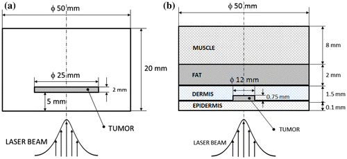
Figure 1(a) and (b) shows, respectively, sketches of the soft-tissue phantom and of the skin model with associated dimensions. Phantom refers to any apparatus or material that mimics the operation and/or physical properties of human systems or tissues. The use of phantoms is an alternative to the use of real tissues. It allows systematic testing and optimization of new methodologies in a controlled way, before testing on animals or humans.[39] As presented in Figure 1(a), the soft-tissue phantom assumed for this work consists of a single region surrounding the disc inclusion that mimics the tumour. Figure 1(b) depicts the skin model considered in this work, composed of epidermis, dermis, fat, muscle and a tumour within the dermis.[18,19,40,41]

Figure 1. Sketches of the cases examined in this work: (a) soft tissue phantom; (b) skin model.

The propagation of laser radiation in the medium is modelled in this work with the δ-P1 diffusion approximation.[42] The computationally cheap diffusion-based models, like the optical diffusion approximation,[43] the P1-approximation [20,21,23] and the δ-P1 diffusion approximation [22,42,44–47], have been used to model light propagation in tissues. On the other hand, the δ-P1 diffusion approximation was shown to provide good agreement with experimental temperature measurements when used to model heat deposition in phantom studies.[22] In fact, the δ-P1 diffusion approximation considers a second-order approximation of the scattering phase function, where it is required that the second moment of the δ-Eddington phase function match that of the Henyey-Greenstein phase function.[46] The laser beam is assumed to be co-axial with the cylindrical medium, so that the problem can be formulated as two dimensional with axial symmetry. The laser incident radiation is assumed to be partially reflected (specular reflection) at the external surface, with reflection coefficient R_sc. The internal surface of the irradiated boundary is assumed to partially and diffusively reflect the incident radiation, with reflectivity characterized by Fresnel’s coefficient A₁, while opacity is assumed for the remaining boundaries. The refractive indexes (n_t) of the different materials are assumed as constant and homogeneous. The mathematical formulation of the radiation problem within the δ-P1 approximation for the problems under study is given below in a general form, using spatially varying optical properties. Therefore, the mathematical formulation holds for both physical models of the phantom and of the skin tissues, given that the same boundary conditions are applied.

The diffuse component of the fluence rate is given by the following boundary value problem [42,45–47]:(1.a) $$\begin{array}{c}\hfill \mathrm{\nabla }·\left[-D\left(r,z\right)\mathrm{\nabla }{\mathrm{\Phi }}_s\left(r,z\right)+\frac{{\mathit{\sigma }}_s^{\prime }\left(r,z\right)g^{\prime }\left(r,z\right)}{{\mathit{\beta }}_{tr}\left(r,z\right)}{\mathrm{\Phi }}_p\left(r,z\right){\widehat{\mathbf{s}}}_c\right]+\mathit{\kappa }\left(r,z\right){\mathrm{\Phi }}_s\left(r,z\right)={\mathit{\sigma }}_s^{\prime }\left(r,z\right){\mathrm{\Phi }}_p\left(r,z\right)\\ \hfill \text{in}0<r<L_r\text{and}0<z<L_z\end{array}$$(1.a) (1.b) $$-D\left(r,z\right)\mathrm{\nabla }{\mathrm{\Phi }}_s\left(r,z\right)·\mathbf{n}+\frac{1}{2A_1}{\mathrm{\Phi }}_s\left(r,z\right)=-\frac{{\mathit{\sigma }}_s^{\prime }\left(r,z\right)g^{\prime }\left(r,z\right)}{{\mathit{\beta }}_{tr}\left(r,z\right)}{\mathrm{\Phi }}_p\left(r,z\right)\text{at}z=0,0<r<L_r$$(1.b) (1.c) $${\mathrm{\Phi }}_s\left(r,z\right)=0\text{at}z=L_z,0<r<L_r$$(1.c) (1.d) $$\mathrm{\nabla }{\mathrm{\Phi }}_s\left(r,z\right)·\mathbf{n}=0\text{at}r=0,0<z<L_z$$(1.d) (1.e) $${\mathrm{\Phi }}_s\left(r,z\right)=0\text{at}r=L_r,0<z<L_z$$(1.e)

where(2.a-e) $$D=\frac{1}{3{\mathit{\beta }}_{tr}};{\mathit{\sigma }}_s^{\prime }=\left(1-g^2\right){\mathit{\sigma }}_s;g^{\prime }=\frac{g}{1+g};A_1=\left(1+R_2\right)/\left(1-R_1\right);{\mathit{\beta }}_{tr}=\mathit{\kappa }+{\mathit{\sigma }}_s\left(1-g\right)$$(2.a-e)

with g being the anisotropy factor of scattering, κ the absorption coefficient, σ_s the scattering coefficient, while R₁ and R₂ are the first and second moments of Fresnel’s reflection coefficient, respectively.

The collimated component of the fluence rate follows the generalized Beer–Lambert’s law and is given by:

(3.a) $${\mathrm{\Phi }}_p\left(r,z\right)={\mathrm{\Phi }}_{0,i}\left(r,z\right)={\mathrm{\Phi }}_{0,i-1}\left(r,d_{i-1}\left(r\right)\right)exp\left[-{\mathit{\beta }}_i^{\prime }\left(z-z_i\right)\right]$$(3.a)

with(3.b) $${\mathit{\beta }}^{\prime }=\mathit{\kappa }+{\mathit{\sigma }}_s^{\prime }$$(3.b)

where the subscript i refers to the layer i, d_i is the thickness of each layer, while z_i and Φ_0,i−1 are the axial position at which the collimated light enters layer i and the collimated fluence rate at this position, respectively. For i = 1 we have:(3.c) $${\mathrm{\Phi }}_{0,1}\left(r,z\right)=\left(1-R_{sc}\right)E_{0}exp\left(-2r^2/r_0^2\right)exp\left(-{\mathit{\beta }}_1^{\prime }z\right)$$(3.c)

where r₀ is the Gaussian beam radius, that is, the radial location where the irradiance falls to 1/e² of the maximum irradiance and is related to the FWHM (Full Width Half Maximum) by(3.d) $$r_0=\frac{\text{FWHM}}{\sqrt{2ln2}}$$(3.d)

The total fluence rate is obtained by adding both diffuse and collimated components, that is,(4) $$\mathrm{\Phi }\left(r,z\right)={\mathrm{\Phi }}_p\left(r,z\right)+{\mathrm{\Phi }}_s\left(r,z\right)$$(4)

The heat transfer problem resulting from the laser irradiation of the medium is modelled in terms of the two-dimensional Pennes’ bioheat transfer equation in cylindrical coordinates with axial symmetry. Despite the limitations in Pennes’ model, which does not take into account changes in the arterial blood temperature, and the availability of other bioheat transfer models (see, for example, reference [24]), there is still no model proven to be sufficiently general and valid for different organs or tissues. In fact, even a pure heat conduction model has been used for applications similar to those considered in the present work.[18] Since the main objective here is the solution of the state estimation problem and not model selection, Pennes’ classical model is used. Both the bottom (irradiated) surface at z = 0 and the top (non-heated) surface at z = L_z are assumed to exchange heat with the surrounding media. For the case involving the soft-tissue phantom, the top and bottom surfaces were assumed to exchange heat by convection and linearized radiation with the ambient. For the skin model, the internal surface is assumed to exchange heat with the deeper tissues at temperature T_int beyond the computational domain, here modelled in terms of convective heat transfer with a coefficient h_int, while the irradiated surface is assumed to be cooled by air in order to avoid overheating of the skin.[24] The heat transfer coefficient h_c and the temperature T_c of the surrounding medium at z = 0 are assumed to vary in the radial direction. Heat transfer is neglected through the lateral surfaces of the medium and the initial temperature is T_s(r,z). The heat transfer problem is then formulated using position-dependent properties as:(5.a) $$\mathit{\rho }\left(r,z\right)c_p\left(r,z\right)\frac{\mathit{\partial }T\left(r,z,t\right)}{\mathit{\partial }t}=\mathrm{\nabla }·\left[k\left(r,z\right)\mathrm{\nabla }T\left(r,z,t\right)\right]+Q\left(r,z\right),0<z<L_z,0<r<L_r,t>0$$(5.a) (5.b) $$k\left(r,z\right)\mathrm{\nabla }T\left(r,z,t\right)·\mathbf{n}+h_c\left(r\right)T\left(r,z,t\right)=h_c\left(r\right)T_c\left(r\right),z=0,0<r<L_r,t>0$$(5.b) (5.c) $$k\left(r,z\right)\mathrm{\nabla }T\left(r,z,t\right)·\mathbf{n}+h_{\text{int}}T\left(r,z,t\right)=h_{\text{int}}{T}_{\text{int}},z=L_z,0<r<L_r,t>0$$(5.c) (5.d) $$\mathrm{\nabla }T\left(r,z,t\right)·\mathbf{n}=0,r=0,0<z<L_z,t>0$$(5.d) (5.e) $$\mathrm{\nabla }T\left(r,z,t\right)·\mathbf{n}=0,r=L_r,0<z<L_z,t>0$$(5.e) (5.f) $$T\left(r,z,t\right)=T_s(r,z)0<z<L_z,0<r<L_r,t=0$$(5.f)

where(6.a) $$Q\left(r,z\right)={\mathit{\rho }}_b{c}_{p,b}{\mathit{\omega }}_b\left(r,z\right)\left[T_b-T\left(r,z,t\right)\right]+Q_{\text{met}}\left(r,z\right)+Q_{\text{laser}}\left(r,z\right)$$(6.a)

The heat source term given by Equation (6.a(6.a) $$Q\left(r,z\right)={\mathit{\rho }}_b{c}_{p,b}{\mathit{\omega }}_b\left(r,z\right)\left[T_b-T\left(r,z,t\right)\right]+Q_{\text{met}}\left(r,z\right)+Q_{\text{laser}}\left(r,z\right)$$(6.a) ) includes the heat source due to laser absorption,(6.b) $$Q_{\text{laser}}\left(r,z\right)=\mathit{\kappa }\left(r,z\right)\mathrm{\Phi }\left(r,z\right)$$(6.b)

but also the heat source due to metabolism and the effect of blood perfusion. The heat source term, Q_laser, induced by the laser radiation is computed from the fluence rate and the absorption coefficient.

3. State estimation problem

The direct (forward) problem associated with the physical problems described above consists in determining the fluence rate distribution and the temperature distribution in the region, from the knowledge of initial and boundary conditions, heat sources, geometry, as well as of optical and thermophysical properties of the tissues.

The inverse problem addressed in this work aims at the estimation of the spatial distribution of the fluence and of transient temperature field in the medium containing the tumour, by accounting for uncertainties on the mathematical model of the physical problem and by assuming local temperature measurements available at one location inside the domain. Such kind of non-stationary inverse problem is in general referred as a state estimation problem, which has many applications in engineering and science (see, for example, references [35–38,48,49]). In state estimation problems, the available measured data are used together with prior knowledge about the physical phenomena and the measuring devices, in order to sequentially produce estimates of the desired dynamic variables, possibly for control purposes.[35–38,48,49] State estimation problems may be written in the form of evolution and observation stochastic models.[35–38,48,49]

We consider a vector x_k, referred to as the state vector, which contains all state variables that describe the system at a given time instant t_k. We further assume known the state evolution model and the observation model, which are defined by the functions f_k and g_k, respectively, so that we can write [35–38,48,49]:(7.a) $${\mathbf{x}}_k={\mathbf{f}}_k\left({\mathbf{x}}_{k-1},\mathit{\theta },{\mathbf{s}}_k\right),k=1,\dots ,M$$(7.a) (7.b) $${\mathbf{z}}_k={\mathbf{g}}_k\left({\mathbf{x}}_k,\mathit{\theta },{\mathbf{v}}_k\right),k=1,\dots ,M$$(7.b)

where $\mathbf{\theta }$ is a vector containing all the non-dynamic parameters of the model, while s_k and v_k represent the noises in the state evolution model and in the observation model, respectively. For the case under study, the state variables contained in the state vector x_k are given by the temperatures and the fluence rates at the discrete points inside the domain that coincide with the centre of finite volumes used in the discretization of the direct problem. Note that the fluence rate is treated as a state variable although not being time dependent, so that inference on its distribution and on the temperature field is simultaneously performed. Note also that the vector $\mathbf{\theta }$ of the non-dynamic parameters contains all thermophysical and optical properties appearing in the mathematical formulations given by Equations (1–6).

The objective of the state estimation problem is to obtain information about the state vector x_k based on the evolution and observation models defined by Equations (7.a(7.a) $${\mathbf{x}}_k={\mathbf{f}}_k\left({\mathbf{x}}_{k-1},\mathit{\theta },{\mathbf{s}}_k\right),k=1,\dots ,M$$(7.a) ) and (7.b).[35–38,48,49] In the case of the filtering problem addressed here, the estimation of the posterior probability distribution $\mathit{\pi }\left({\mathbf{x}}_k|{\mathbf{z}}_{1:k},\mathbf{\theta }\right)$ is of interest, that is, the non-dynamic model parameters are treated as deterministically known. In other words, the thermophysical and optical properties appearing in Equations (1–6) are fixed deterministically. With such an approach, uncertainties on the parameters are implicitly embodied in s_k and v_k. A different approach might be the estimation of the joint posterior probability distribution $\mathit{\pi }\left({\mathbf{x}}_k,\mathbf{\theta }|{\mathbf{z}}_{1:k}\right)$ of the state variables and of the non-dynamic parameters.[49,50] However, the computational cost for the particle filter solution can be high in these cases.[30] We also assume that the probability density $\mathit{\pi }\left({\mathbf{x}}_0|{\mathbf{z}}_0,\mathbf{\theta }\right)=\mathit{\pi }\left({\mathbf{x}}_0\right)$ at the initial state t = t₀ is available. Given the state evolution–observation model of Equations (7(7.a) $${\mathbf{x}}_k={\mathbf{f}}_k\left({\mathbf{x}}_{k-1},\mathit{\theta },{\mathbf{s}}_k\right),k=1,\dots ,M$$(7.a) .a and 7.b) and the initial probability distribution of the states, the estimation of the posterior probability distribution $\mathit{\pi }\left({\mathbf{x}}_k|{\mathbf{z}}_{1:k},\mathbf{\theta }\right)$ is achieved in two steps with Bayesian filters: prediction and update.[35–38,49,50] The state evolution model is used to predict the state of the system at time instant t_k, while the observation model, which relates the states variables with observable variables, is used to compute the likelihood with available measurements at time instant t_k.

Among Bayesian filters, the Kalman filter family, as applied to non-linear problems, is based on a Gaussian approximation of the sought posterior probability distribution and their accuracy can be seriously affected when the posterior density is multi-modal or strongly peaked.[48,49] Particle filters, or sequential Monte Carlo, are more general and do not rely on any prior assumption on the posterior probability distribution. Therefore, they can be applied to non-linear evolution and observation models with non-Gaussian noises.[35–38,48,49] The particle filter method is a Monte Carlo technique for the solution of state estimation problems, in which the posterior probability density function is represented by a set of random samples (particles) with associated weights. As the number of samples becomes large, the Monte Carlo characterization becomes an equivalent representation of the posterior probability density function and the solution approaches the optimal Bayesian estimate. The particle filter algorithms generally make use of an importance density, which is a probability density function proposed to represent another one that cannot be exactly computed, that is, the sought posterior density in the present case. Then, samples are drawn from the importance density instead of the actual density.[35–38,48,49]

Let ${\mathbf{x}}_{0:k}^i,i=1,\dots ,N$ be the particles with associated weights $w_k^i,i=1,\dots ,N$ and ${\mathbf{x}}_{0:k}$ be the set of all state variables up to t_k, where N is the number of particles. The weights are normalized so that ${\sum }_{i=1}^N{w}_k^i=1$. The posterior probability distribution of the state variables at the time instant t_k can be discretely approximated by [35–37]:(8) $$\mathit{\pi }\left({\mathbf{x}}_k|{\mathbf{z}}_{1:k},\mathit{\theta }\right)\approx \sum _{i=1}^N{w}_k^i\mathit{\delta }\left({\mathbf{x}}_k-{\mathbf{x}}_k^i\right)$$(8)

where $\mathit{\delta }\left(.\right)$ is the Dirac delta function and $w_k^i$ represents the weights of each particle i.

The most popular particle filters are the Sampling Importance Resampling (SIR) [35–37] and the Auxiliary Sampling Importance Resampling (ASIR).[35–37,51] Particle filters make use of a resampling step, in which particles with small weights are eliminated and particles with large weights are replicated. However, the sequential application of the resampling step in the SIR filter may introduce a loss of diversity. The ASIR filter was introduced in [51] as a variant of the SIR filter, in which an attempt is made to overcome the loss of diversity by performing the resampling step at time t_k−1, with the available measurements at time t_k.[35,36] In other words, the idea is to mimic the availability of the optimal importance density $\mathit{\pi }\left({\mathbf{x}}_k^i|{\mathbf{x}}_{k-1}^i,\mathbf{\theta },{\mathbf{z}}_k\right)$.[52] The resampling is based on some point estimate ${\mathbf{\mu }}_k^i$ that characterizes $\mathit{\pi }\left({\mathbf{x}}_k^i|{\mathbf{x}}_{k-1}^i,\mathbf{\theta }\right)$, which can be the mean, the mode, the median or simply a sample of $\mathit{\pi }\left({\mathbf{x}}_k^i|{\mathbf{x}}_{k-1}^i,\mathbf{\theta }\right)$. The ASIR [35,36] version of the particle filter, summarized in Table 1, is used in this paper for the estimation of the posterior probability distribution $\mathit{\pi }\left({\mathbf{x}}_k|{\mathbf{z}}_{1:k},\mathbf{\theta }\right)$. In this work, the resampling step was based on the mean of the prior density $\mathit{\pi }\left({\mathbf{x}}_k^i|{\mathbf{x}}_{k-1}^i,\mathbf{\theta }\right)$.

Table 1. Auxiliary sampling importance resampling (ASIR) algorithm.[28,29]

Step 1

For i = 1, …, N draw new particles ${\mathbf{x}}_k^i$ from the prior density π (xk|${\mathbf{x}}_{k-1}^i$, θ) by solving the forward problem for ${\mathbf{x}}_{k-1}^i$ and θ. Then, calculate some characterization ${\mathbf{\mu }}_k^i$ of xk, given ${\mathbf{x}}_{k-1}^i$ and use the likelihood density to calculate the corresponding weights $w_k^i$ = π(${\mathbf{z}}_k^{\text{meas}}$|${\mathbf{\mu }}_k^i$,θ)$w_{k-1}^i$.

Step 2

Calculate the total weight t = Σi$w_k^i$ and then normalize the particle weights, that is, for i = 1, …, N let $w_k^i$ = $t^{-1}{w}_k^i$.

Step 3

Resample the particles as follows:

Construct the cumulative sum of weights (CSW) by computing ci = ci−1 + $w_k^i$ for i = 1, …, N, with c0 = 0

Let i = 1 and draw a starting point u1 from the uniform distribution U[0,N^−1]

For j = 1, …, N

Move along the CSW by making uj = u1 + N^−1(j − 1)

While uj  > ci make i = i + 1

Assign samples ${\mathbf{x}}_{k-1}^j={\mathbf{x}}_{k-1}^i$

Assign sample weights $w_k^j$ = N^−1

Assign parent i^j = i

Step 4

For j =1, …, N draw particles x^jk from the prior density π (xk|${\mathbf{x}}_{k-1}^{ij}$, θ), by solving the forward problem using the parent i^j, and then use the likelihood density to calculate the correspondent weights $w_k^j$ = π${\mathbf{z}}_k^{\text{meas}}$|(${\mathbf{x}}_k^j$, θ)/π (${\mathbf{z}}_k^{\text{meas}}$|${\mathbf{\mu }}_k^{ij}$, θ).

Step 5

Calculate the total weight t = Σj $w_k^j$ and then normalize the particle weights; that is, for j = 1, …, N let $w_k^j$ = $t^{-1}{w}_k^j$ .

4. Results and discussions

The results obtained for the state estimation problem for the two test-cases examined in this work are now presented and discussed. For the solution of the direct coupled radiation – bioheat transfer problem, a finite volume code, based on the alternating direction implicit method (ADI), was developed.[44] Code and solution verifications were performed by comparing the solution of the light diffusion problem to the analytical solution for the case of a semi-infinite homogeneous medium, while the bioheat transfer problem was verified against the solution obtained with the COMSOL Multiphysics commercial software.[44]

For the solution of the state estimation problem, the evolution model for temperature was obtained from the finite volume ADI discretization. The noise in the evolution model for temperature was assumed as additive, uncorrelated, Gaussian, with zero mean and a standard deviation σ_T = 0.5 °C. The evolution model for the fluence rate distribution was taken in the form of a random walk, with additive, uncorrelated and Gaussian noise, with zero mean and a standard deviation σ_Φ = 1% of its deterministic value. Both evolution models of the temperature and of the fluence rate are given by Equation (9(9) $${\mathbf{x}}_{k+1}^{}={\mathbf{f}}_{k+1}^{}\left({\mathbf{x}}_k\right)+{\mathit{\epsilon }}_{k+1}^{}\Rightarrow \left\{\begin{array}{cc}{\mathrm{\Phi }}_{k+1}\hfill & ={\mathrm{\Phi }}_k+{\mathit{\sigma }}_{\mathrm{\Phi }}{\mathit{\epsilon }}_{{}_{k+1}}^{\mathrm{\Phi }}\hfill \\ {\mathbf{T}}_{k+1}\hfill & ={\mathbf{f}}_{k+1}^T\left({\mathbf{T}}_k,{\mathrm{\Phi }}_{k+1}\right)+{\mathit{\sigma }}_T{\mathit{\epsilon }}_{{}_{k+1}}^T\hfill \end{array}\right.$$(9) ), where ${\mathbf{\epsilon }}_{k+1}$ is a Gaussian variable with zero mean and unitary standard deviation.(9) $${\mathbf{x}}_{k+1}^{}={\mathbf{f}}_{k+1}^{}\left({\mathbf{x}}_k\right)+{\mathit{\epsilon }}_{k+1}^{}\Rightarrow \left\{\begin{array}{cc}{\mathrm{\Phi }}_{k+1}\hfill & ={\mathrm{\Phi }}_k+{\mathit{\sigma }}_{\mathrm{\Phi }}{\mathit{\epsilon }}_{{}_{k+1}}^{\mathrm{\Phi }}\hfill \\ {\mathbf{T}}_{k+1}\hfill & ={\mathbf{f}}_{k+1}^T\left({\mathbf{T}}_k,{\mathrm{\Phi }}_{k+1}\right)+{\mathit{\sigma }}_T{\mathit{\epsilon }}_{{}_{k+1}}^T\hfill \end{array}\right.$$(9)

Transient temperature measurements taken at one single position inside the medium were assumed available for the inverse analysis. The measurements were simulated, for each test-case, from the solution of the direct problem, which was obtained on a refined finite volume grid in order to avoid an inverse crime.[37] For the case involving the phantom, the simulated measurements were generated on a grid with 200 volumes in the radial direction, 300 volumes in the axial direction and time step of 1 s. For the skin model, the grid used for simulating the measurements consisted of 180 volumes in the radial direction, 300 volumes in the axial direction and time step of 1 s. Simulated measurement errors were additive, Gaussian, uncorrelated, with zero mean and a constant standard deviation σ_meas = 0.5 °C. Thus, the likelihood function used for the calculation of the weights $w_k^i$ for each particle (see Table 1) is given by:(10) $$\mathit{\pi }\left({\mathbf{z}}_{{}_k}^{\text{meas}}|{\mathbf{x}}_{{}_k}^i,\mathit{\theta }\right)\propto exp\left\{-\frac{1}{2}\frac{{\left[{\mathbf{z}}_{{}_k}^{\text{meas}}-{\mathbf{z}}_{{}_k}^{}({\mathbf{x}}_{{}_k}^i,\mathit{\theta })\right]}^2}{{\mathit{\sigma }}_{\text{meas}}^2}\right\}$$(10)

where ${\mathbf{z}}_{{}_k}^{\text{meas}}$ represents the temperature measurements at time t_k, while ${\mathbf{z}}_{{}_k}^{}({\mathbf{x}}_{{}_k}^i,\mathbf{\theta })$ represents the predicted temperatures at the same time instant obtained with the particle ${\mathbf{x}}_{{}_k}^i$ and the parameter vector θ. The ASIR particle filter was used for the solution of the state estimation problem with 100 and 250 particles, as discussed below.

4.1. State estimation for the soft-tissue phantom

For this test-case, the disc region that mimics the tumour is supposed to be located within a region made of polyvinyl chloride plastisol (PVC-P).[39] While the thermophysical properties for PVC-P were measured,[39] its optical properties were assumed to match those of soft tissues.[53,54] Table 2 shows the thermophysical and optical properties of PVC-P at λ = 810 nm that were used in the calculations. The thickness and the radius of the phantom were set, respectively, to 20 and 25 mm, while the tumour, located at a depth of 5 mm from the irradiated surface, was considered with a thickness of 2 mm and radius of 12.5 mm (see Figure 1(a)). The phantom was assumed to be initially in thermal equilibrium with the ambient at T_s = 25 °C and the heat transfer coefficient at the irradiated boundary was taken as h_c = 10 W/mK. A much higher heat transfer coefficient (h_int = 1000 W/mK) was assumed for the non-heated boundary (z = L_z), in order to approximate a prescribed constant temperature boundary condition. The region containing the tumour was supposed to be made of PVC-P but loaded with gold nanorods of effective radius 11.43 nm and aspect ratio 3.9, which have a peak of plasmonic resonance at 797 nm, corresponding to an absorption cross section C_abs = 2.2128 × 10⁻¹⁴ m² and a scattering cross section C_sca = 1.7286 × 10⁻¹⁵ m².[55] The volumetric optical properties of the gold nanorods shown in Table 3 were calculated by assuming a concentration of nanoparticles f_v = 8 × 10¹⁵ m⁻³. The optical properties of the region loaded with the gold nanorods were given by Equations (11.a) and (11.b). It is assumed here that only the absorption and the scattering coefficients are affected by the inclusion of the nanoparticles, that is,(11.a,b) $${\mathit{\kappa }}_{\text{tot}}=\mathit{\kappa }+C_{\text{abs}}{f}_v{\mathit{\sigma }}_{s,\text{tot}}={\mathit{\sigma }}_s+C_{\text{sca}}{f}_v$$(11.a,b)

Table 2. Thermophysical and optical properties of the PVCP phantom.[32,44,45]

Density ρ (kg/m^3)	Specific heat cp (kJ/kgK)	Thermal conductivity k (W/mK)	Absorption coefficient κ (m^−1)	Scattering coefficient σs(m^−1)	Scattering anisotropy factor g
995.1	1.79	0.15	2	12,000	0.9

Table 3. Optical properties of region loaded with gold nanorods.

Concentration of nanoparticles (m^−3)	8 × 10^15
κ (m^−1)	179.02
σs (m^−1)	12,013.83

The simulations were carried out by assuming a laser output power of 0.35 W under constant illumination during 180 s, with a Gaussian-shaped beam with r₀ = 4.25 mm. For the results presented below for the inverse problem, the finite volume grid was generated with 100 volumes in the radial direction and 150 volumes in the axial direction. The time step used to march the solution in time was 1 s. Transient temperature measurements at the position (r = 2 mm, z = 6 mm), with a frequency of one measurement every 1 s, were assumed available for the inverse analysis.

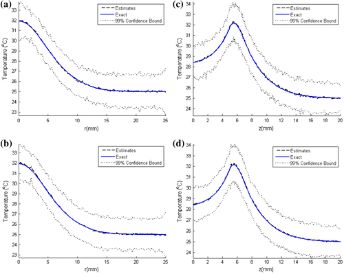
Figure 2 shows a comparison of the estimated temperature distributions with the exact ones, at selected time instants, for N = 100 and 250 particles. Such results reveal that quite accurate estimates were obtained with the present approach; the estimated temperature distributions are in excellent agreement with the exact ones for both N = 100 and 250 particles. This can also be seen in Figure 3(a)–(d), where the temperature distribution is shown along the radial direction for a line at z = 6 mm and along the axial direction at the centerline. Note in these figures that there is no significant difference between the confidence bounds of the estimated temperature distribution when the particle number was increased from N = 100 to 250, that is, the confidence bounds have converged.

Figure 2. Exact and estimated temperature distribution at selected times with N = 100 particles and with N = 250 particles.

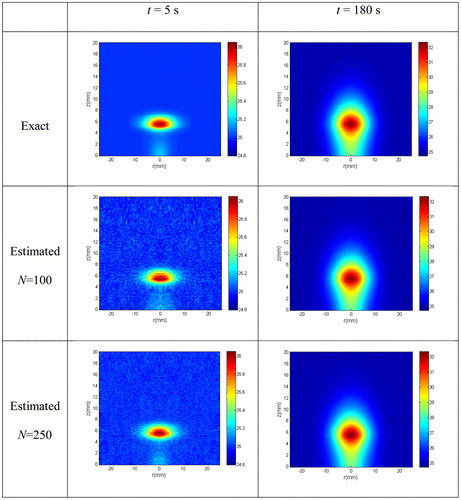
Figure 3. Estimated and exact temperature distribution at t = 180 s: (Left) along the radius for a line at z = 6 mm of the inclusion with N = 100 particles (a) and N = 250 particles (b); (Right) along the centerline with N = 100 particles (c) and N = 250 particles (d).

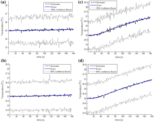
In order to further assess the accuracy of the estimated temperatures, we compare in Figure 4, for N = 100 and 250 particles, the estimated and the exact transient temperatures at the measurement position (r = 2 mm, z = 6 mm). The simulated temperature measurements are also included in Figure 4. It can be noticed in this figure that the estimated temperatures are in better agreement with the exact ones than the measurements are. Similar results are presented in Figure 5 at two other positions, (r = 15 mm, z = 6 mm) and (r = 0 mm, z = 10 mm), where no measurements were taken. Figure 5 shows that, even at locations where no measurements were taken, the estimated temperatures are in very good agreement with the exact ones. As noticed above, the convergence of the confidence bounds of the estimates can be observed in Figures 4 and 5 where the number of particles was increased from N = 100 to 250 particles.

Figure 4. Comparison of the estimated and exact transient temperature variations with the temperature measurements at the sensor position (r = 2 mm, z = 6 mm): (a) N = 100 particles; (b) N = 250 particles.

Figure 5. Estimated and exact transient temperature variations: (Left) at (r = 15 mm, z = 6 mm) with N = 100 particles (a) and N = 250 particles (b); (Right) at (r = 0 mm, z = 10 mm) with N = 100 particles (c) and N = 250 particles (d).

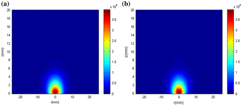
In this work, the fluence rate was treated as a state variable, so that inference on its distribution was obtained together with inference on the temperature. Figure 6 shows the exact fluence rate distribution and the estimated fluence rate distribution at t = 180 s, obtained with N = 250 particles. As it can be seen, accurate estimates of the fluence rate distribution were obtained.

Figure 6. (a) Exact fluence rate distribution; (b) Fluence rate distribution estimated with N = 250 particles.

4.2. State estimation for the skin model

The initial distribution of the temperature in the skin tissues was obtained from the solution of the steady-state bioheat transfer equation, given by Equations (5) and (6), with the parameters presented in Table 4, but without laser irradiation, that is, Q_laser = 0 W/m³ in Equation (6.a(6.a) $$Q\left(r,z\right)={\mathit{\rho }}_b{c}_{p,b}{\mathit{\omega }}_b\left(r,z\right)\left[T_b-T\left(r,z,t\right)\right]+Q_{\text{met}}\left(r,z\right)+Q_{\text{laser}}\left(r,z\right)$$(6.a) ).[40,41,56] The diameter of the sample was set to 50 mm, while the tumour dimensions were set to 12 mm in diameter and 0.75 mm in thickness (see Figure 1(b)). The optical properties of the tumour were taken equal to those of the dermis. In addition, the scattering coefficients presented in Table 4 were calculated from their reduced scattering coefficient reported in [56], by assuming an anisotropy factor of 0.9 for epidermis, dermis and fat, with g = 0.93 for the muscle. The first and second moments of Fresnel’s reflection coefficients for the air–tissue interface, with tissue refractive index n_t = 1.3, are given by 0.565 and 0.429, respectively.[57] The heat transfer coefficient to the ambient was set to h_c = 10 W/m² K and the heat transfer coefficient to deeper tissues was taken as h_int = 50 W/m² K.

Table 4. Thermophysical and optical properties of tissues.[33,34,47]

Tissue	Epidermis	Tumour	Dermis	Fat	Muscle
Thickness, (mm)	0.1	0.75	1.5	2	8
ρ (kg/m^3)	1200	1030	1200	1000	1085
cp (J/kg K)	3589	3852	3300	2674	3800
k (W/m K)	0.235	0.558	0.445	0.185	0.51
Qmet (W/m^3)	0	3680	368.1	368.3	684.2
ωb (s^−1)	0	63 × 10^−4	2 × 10^−4	10^−4	27 × 10^−4
κ (m^−1)	35	122	122	108	54
σs (m^−1)	21,270	22,500	22,500	20,200	6670

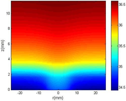
The obtained initial temperature distribution is shown in Figure 7. Note in this figure that, as expected, the temperature decays from the internal tissues to the superficial tissues due to heat transfer to the surrounding environment. Note also that, due to the higher metabolic heat source of the tumour, the surface temperature is slightly higher in the tumour region and decays at remote distance from the tumour. Such an abnormal skin surface temperature has been suggested as an indication of the presence of skin tumours.[40,41,58]

Figure 7. Initial temperature distribution.

The initial temperature presented by Figure 7 was used for the state estimation problem, but with the tumour supposedly loaded with gold nanorods of effective radius 11.43 nm, aspect ratio 3.9 and concentration of 3 × 10¹⁵ m⁻³. The optical properties of the tumour-containing gold nanorods, computed with Equations (11(11.a,b) $${\mathit{\kappa }}_{\text{tot}}=\mathit{\kappa }+C_{\text{abs}}{f}_v{\mathit{\sigma }}_{s,\text{tot}}={\mathit{\sigma }}_s+C_{\text{sca}}{f}_v$$(11.a,b) .a and 11(11.a,b) $${\mathit{\kappa }}_{\text{tot}}=\mathit{\kappa }+C_{\text{abs}}{f}_v{\mathit{\sigma }}_{s,\text{tot}}={\mathit{\sigma }}_s+C_{\text{sca}}{f}_v$$(11.a,b) .b), are shown by Table 5. Again, it is assumed here that only the absorption and the scattering coefficients are affected by the inclusion of the nanoparticles. The imposed laser flux (λ = 800 nm) at the surface of the body was assumed to be of constant magnitude 1.5 W/cm², with r₀ = 5.9 mm and irradiation time of 20 s. In order to avoid an overheating of the skin surface during the hyperthermia treatment we assume, as in [24], a heat transfer coefficient h_c = 500 W/m² K to a medium at T_c = 35 °C for radial positions smaller than the tumour radius. For the regions beyond the tumour radius, we assume h_c = 10 W/m² K and T_c = 25 °C.

Table 5. Optical properties of the tumour-containing gold nanorods.

Concentration of nanoparticles (m^−3)	3 × 10^15
κ (m^−1)	188.38
σs (m^−1)	22,505.19

To find out the magnitude of thermal damage, the Arrhenius thermal damage function can be used, which is defined by [25]:(12) $$\mathrm{\Omega }\left(r,z,t\right)=A\underset{t^{\prime }=0}{\overset{t}{\int }}exp\left(-\frac{E_a}{RT\left(r,z,t^{\prime }\right)}\right)\text{d}{t}^{\prime }$$(12)

where A is the frequency factor [1/s], E_a is the activation energy [J/mol], R is the universal gas constant and T is the absolute temperature [K]. Since the thermal damage function is an explicit function of the temperature, it is possible to propagate the uncertainties associated with the estimated temperatures in its calculation. Therefore, the Arrhenius thermal damage function was implemented within the particle filter algorithm, so that, at each time instant t_k, it was evaluated for each particle. For the calculation of the thermal damage function, the frequency factor A, and the activation energy E_a were taken as 1.8 × 10⁵¹ s⁻¹ and 3.27 × 10⁵ J/mol, respectively.[59]

For the results presented below for the inverse problem, a finite volume grid with 90 volumes in the radial direction, 150 volumes in the axial direction and a time step of 1 s was used. Transient temperature measurements at the position (r = 0.5 mm, z = 0.7 mm) inside the tumour, taken at a rate of one measurement per second, were assumed available for the inverse analysis. We compare in Figure 8 the estimated temperature distributions with the exact ones, at selected time instants for N = 100 and 250 particles. Note that, for both numbers of particles, the estimated temperature distributions are very similar to the exact ones. The obtained results demonstrate that, such as for the case involving the phantom, quite accurate estimates were obtained with the ASIR filter for this case involving the skin model.

Figure 8. Exact and estimated temperature distribution at selected times with N = 100 particles and N = 250 particles.

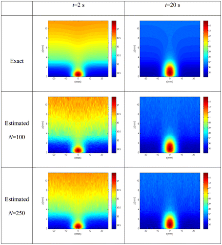
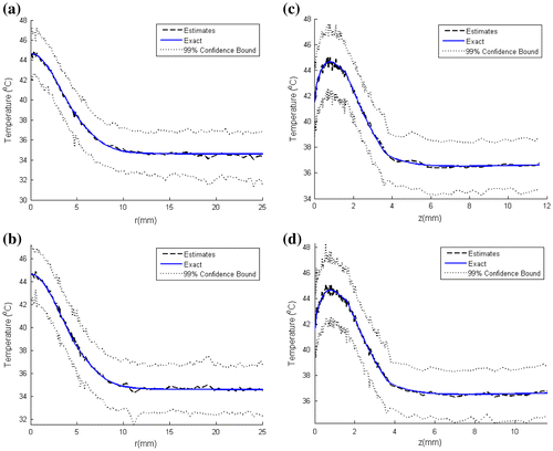
Figure 9 presents the exact and estimated temperatures at t = 20 s along the radial direction at z = 0.7 mm and along the axis of the cylinder, for N = 100 and 250 particles. Note in these figures that, the estimated means agree with the exact temperatures for both N = 100 and 250 particles. Note also that, at the graph scale, there is no significant difference in the confidence bounds when the number of particles is increased from N = 100 to 250 particles.

Figure 9. Estimated and exact temperature distribution at t = 20 s: (Left) along the radius for a line at z = 0.7 mm with N = 100 particles (a) and N = 250 particles (b); (Right) along the centerline with N = 100 particles (c) and N = 250 particles (d).

Figures 10 and 11 present the estimated and the exact transient temperatures at the measurement position (r = 0.5 mm, z = 0.7 mm) and at two other positions (r = 8 mm, z = 0.7 mm and r = 0 mm, z = 3 mm) where no measurements were taken, respectively. The simulated temperature measurements were also included in Figure 10. Figures 10 and 11 show that the estimated temperatures are in very good agreement with the exact ones. In special, Figure 11 reveals that such is the case even at locations where no measurements are available. Finally, we present in Figure 12 the exact and estimated fluence rate distribution at t = 20 s, obtained with N = 250 particles. One can notice in this figure that the fluence rate distribution can be quite accurately estimated.

Figure 10. Comparison of the estimated and exact transient temperature variations with the temperature measurements at the sensor position (r = 0.5 mm, z = 0.7 mm): N = 100 particles (a); N = 250 particles (b).

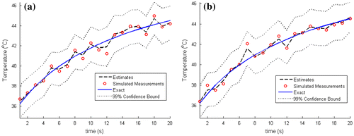
Figure 11. Estimated and exact transient temperature variations: (Left) at (r = 6 mm, z = 0.7 mm) with N = 100 particles (a) and N = 250 particles (b); (Right) at (r = 0 mm, z = 3 mm) with N = 100 particles (c) and N = 250 particles (d).

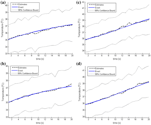
Figure 12. (a) Exact fluence rate distribution; (b) Fluence rate distribution estimated with N = 250 particles.

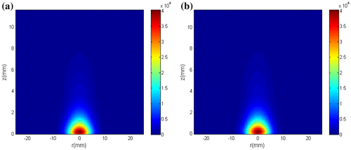
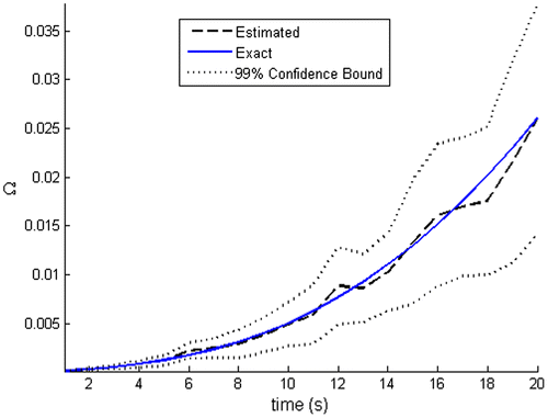
Figure 13 presents a comparison of the thermal damage function calculated with the exact temperatures, with the one obtained with N = 250 particles, at the time instant t = 20 s. It can be noticed that the thermal damage is larger in the tumour region. A comparison of the transient behaviour of the thermal damage calculated with the exact temperatures and with the estimated temperatures at the sensor position is presented in Figure 14, with associated confidence bounds. One can notice that a good agreement between exact and calculated thermal damage is obtained. Note also in this figure that the associated confidence bounds are wider for increasing time, as a consequence of the propagation of the uncertainties.

Figure 13. (a) Exact thermal damage distribution; (b) Estimated thermal damage distribution with N = 250 particles.

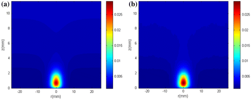
Figure 14. Comparison of the transient variation of the thermal damage calculated with the exact and estimated temperatures at the position (r = 0.5 mm, z = 0.7 mm).

5. Conclusions

This work has dealt with the inverse estimation of the transient temperature distribution, as well as of the fluence rate distribution, in laser-induced hyperthermia therapy of cancer enhanced with photo-absorbing nanoparticles, using transient temperature measurements taken at one single sensor inside the domain. The ASIR particle filter was successfully applied for the solution of the present state estimation problem, even under conditions of large uncertainties in the evolution and observations models. Such conclusion applies both to the case of a phantom and a skin cancer. The use of more elaborate models for light radiation in tissues and bio heat transfer can be easily accommodated into the methodology applied in this work. On the other hand, we demonstrate that the ASIR algorithm of particle filter is capable of dealing with the state estimation problem for the hyperthermia treatment of cancer with infrared remote heating, which was the main objective of this paper. The results obtained in this work show that the proposed methodology can be used for the hyperthermia treatment planning, and possibly be coupled to control algorithms, in order to handle the uncertainties involved in practice.

Nomenclature
cp	=	specific heat
D	=	diffusion coefficient for the δ-P1 approximation
E0	=	maximum laser radiation flux imposed at z = 0
g	=	anisotropy scattering factor
k	=	thermal conductivity
L	=	radius of the cylinder
Lz	=	thickness of the cylinder
N	=	number of particles
n	=	unity vector normal to the boundary
Q	=	volumetric heat source
r, z	=	spatial variables
r0	=	Gaussian radius of the laser beam
R1, R2	=	first and second moments of Fresnel’s reflection coefficient, respectively
Rsc	=	specular reflection coefficient at z = 0
T	=	temperature
Ts	=	initial temperature
t	=	time
wk	=	particle weight
${\widehat{\mathbf{s}}}_c$	=	direction of propagation of the collimated laser beam
sk, vk	=	noises in the state evolution model and in the observation model, respectively
xk	=	state vector

Greeks
${\mathit{\beta }}_i^{\prime }$	=	reduced total attenuation coefficient of layer i
βtr	=	transport attenuation coefficient
$\mathbf{\theta }$	=	vector containing all the non-dynamic parameters of the model
κ	=	absorption coefficient
λ	=	wavelength
ρ	=	density
σs	=	scattering coefficient
${\mathit{\sigma }}_s^{\prime }$	=	reduced scattering coefficient
Φp	=	collimated component of the fluence rate
Φs	=	diffusive fluence rate
Φ	=	total fluence rate
ω	=	perfusion coefficient
Ω	=	thermal damage function

Subscripts
b	=	blood
i	=	layer i
met	=	metabolic
k	=	time instant

Superscripts
i	=	particle number

Funding

This work was supported by Conselho Nacional de Desenvolvimento Científico e Tecnológico, Coordenação de Aperfeiçoamento de Pessoal de Nível Superior, CONICET, FAPERJ.

Disclosure statement

No potential conflict of interest was reported by the authors.

Acknowledgements

The authors are thankful for the support provided by CNPq, CAPES and FAPERJ, Brazilian agencies for the fostering of science, as well as from CONICET of Argentina.

References

- Habash RWY, Bansal R, Krewski D, et al. Thermal Therapy Part 1: An Introduction to Thermal Therapy. Crit. Rev. Biomed. Eng. 2011;34:459–489.
- Chatterjee DK, Krishnan S. Gold Nanoparticle-mediated Hyperthermia in Cancer Therapy. In: Cho HS, Krishnan S, editors. Cancer nanotechnology, principles and applications in radiation oncology. chap. 14. Boca Raton (FL): CRC Press; 2013. p. 171–182.
- Chatterjee DK, Diagaradjane P, Krishnan S. Nanoparticle-mediated hyperthermia in cancer therapy. Therapeutic Delivery. 2011;2:1001–1014.10.4155/tde.11.72
- Kampinga HH. Cell biological effects of hyperthermia alone or combined with radiation or drugs: a short introduction to newcomers in the field. Int. J. Hyperth. 2006;22:191–196.10.1080/02656730500532028
- Bayazitoglu Y, Kheradmand S, Tullius TK. An overview of nanoparticle assisted laser therapy. Int. J. Heat Mass Transf. 2013;67:469–486.10.1016/j.ijheatmasstransfer.2013.08.018
- Huang X, El-Sayed MA. Gold nanoparticles: optical properties and implementations in cancer diagnosis and photothermal therapy. J. Adv. Res. 2010;1:13–28.10.1016/j.jare.2010.02.002
- Khlebtsov NG, Dykman LA. Optical properties and biomedical applications of plasmonic nanoparticles. J. Quant. Spectr. Radiat. Transfer. 2010;111:1–35.10.1016/j.jqsrt.2009.07.012
- Hirsch LR, Stafford RJ, Bankson JA, et al. Nanoshell-mediated near-infrared thermal therapy of tumors under magnetic resonance guidance. Proc. Nat. Acad. Sci. USA. 2003;100:13549–13554.10.1073/pnas.2232479100
- El-Sayed IH, Huang X, El-Sayed MA. Surface plasmon resonance scattering and absorption of anti-EGFR antibody conjugated gold nanoparticles in cancer diagnostics: applications in oral cancer. Nano Lett. 2005;5:829–834.10.1021/nl050074e
- O’Neal DP, Hirsch LR, Halas NJ, et al. Photo-thermal tumor ablation in mice using near infrared-absorbing nanoparticles. Cancer Lett. 2004;209:171–176.10.1016/j.canlet.2004.02.004
- Clinicaltrials.gov: Pilot study of AuroLase(tm) therapy in refractory and/or recurrent tumors of the head and neck, in, National Institute of Health. 2010. Available from: http://clinicaltrials.gov/ct2/show/NCT00848042. September 2015.
- Rengan AK, Bukhari AB, Pradhan A, et al. In vivo analysis of biodegradable liposome gold nanoparticles as efficient agents for photothermal therapy of cancer. Nano Lett. 2015;15:842–848.10.1021/nl5045378
- Wang Q, Xie L, He Z, et al. Biodegradable magnesium nanoparticle-enhanced laser hyperthermia therapy. Int. J. Nanomed. 2012;7:4715–4725.
- Jung T, Grune T. Experimental basis for discriminating between thermal and athermal effects of water-filtered infrared A irradiation. Ann. N. Y. Acad. Sci. 2012;1259:33–38.10.1111/nyas.2012.1259.issue-1
- Kelleher DK, Thews O, Rzeznik J, et al. Water filtered infrared-A-radiation: a novel technique for localized hyperthermia in combination with bacteriochlorophyll-based photodynamic therapy. Int. J. Hyperthermia. 1999;15:467–474.
- Notter M, Piazena H, Muller W, et al. Low dose re-irradiation & thermography controlled wIRA hyperthermia in extended recurrent breast cancer. Proceedings of 31st Annual Meeting of the Society for Thermal Medicine; Minneapolis (MN); 2014.
- Piazena H, Kelleher DK. Effects of infrared-A irradiation on skin: discrepancies in published data highlight the need for an exact consideration of physical and photobiological laws and appropriate experimental settings. Photochem. Photobiol. 2010;86:687–705.10.1111/php.2010.86.issue-3
- Dombrovsky LA, Timchenko V, Pathak C, et al. Radiative heating of superficial human tissues with the use of water-filtered infrared-A radiation: a computational modeling. Int. J. Heat Mass Transfer. 2015;85:311–320.10.1016/j.ijheatmasstransfer.2015.01.133
- Dombrovsky LA, Timchenko V, Jackson M, et al. A combined transient thermal model for laser hyperthermia of tumors with embedded gold nanoshells. Int. J. Heat Mass Transfer. 2011;54:5459–5469.10.1016/j.ijheatmasstransfer.2011.07.045
- Vera J, Bayazitoglu Y. Gold nanoshell density variation with laser power for induced hyperthermia. Int. J. Heat Mass Transfer. 2009;52:564–573.10.1016/j.ijheatmasstransfer.2008.06.036
- Vera J, Bayazitoglu Y. A note on laser penetration in nanoshell deposited tissue. Int. J. Heat Mass Transfer. 2009;52:3402–3406.10.1016/j.ijheatmasstransfer.2009.02.014
- Elliott AM, Schwartz J, Wang J, et al. Quantitative comparison of delta P1 versus optical diffusion approximations for modeling near-infrared gold nanoshell heating. Med. Phys. 2009;36:1351–1358.10.1118/1.3056456
- Dombrovsky LA, Randrianalisoa JH, Lipinski W, et al. Simplified approaches to radiative transfer simulations in laser-induced hyperthermia of superficial tumors. Comput. Thermal Sci. 2013;5:521–530.10.1615/ComputThermalScien.v5.i6
- Dombrovsky LA, Timchenko V, Jackson M. Indirect heating strategy for laser induced hyperthermia: an advanced thermal model. Int. J. Heat Mass Transfer. 2012;55:4688–4700.10.1016/j.ijheatmasstransfer.2012.04.029
- Fuentes D, Oden JT, Diller KR, et al. Computational modeling and real-time control of patient-specific laser treatment of cancer. Ann. Biomed. Eng. 2009;37:763–782.10.1007/s10439-008-9631-8
- Gellermann J, Hildebrandt B, Issels R, et al. Noninvasive magnetic resonance thermography of soft tissue sarcomas during regional hyperthermia. Cancer. 2006;107:1373–1382.10.1002/(ISSN)1097-0142
- Feng Y, Fuentes D. Model-based planning and real-time predictive control for laser-induced thermal therapy. Int. J. Hyperth. 2011;27:751–761.10.3109/02656736.2011.611962
- Liu J. Uncertainty analysis for temperature prediction of biological bodies subject to randomly spatial heating. J. Biomech. 2001;34:1637–1642.10.1016/S0021-9290(01)00134-8
- Liu J. Ways toward targeted freezing or heating tumor: precisely managing the heat delivery inside biological systems. Proceedings of 15th Int. Heat Trans. Conf., IHTC15-KN16; 2014, 1–25.
- Lamien B, Orlande HRB, Eliçabe G, et al. State estimation problem in hyperthermia treatment of tumors loaded with nanoparticles. Proc. of 15th Int. Heat Trans. Conf., IHTC15-8772; 2014, 1–14.
- dos Santos I, Haemmerich D, Schutt D, et al. Probabilistic finite element analysis of radiofrequency liver ablation using the unscented transform. Phys. Med. Biol. 2009;54:627–640.10.1088/0031-9155/54/3/010
- Greef DM, Kok HP, Correia D, et al. Uncertainty in hyperthermia treatment planning: the need for robust system design. Phys. Med. Biol. 2011;56:3233–3250.10.1088/0031-9155/56/11/005
- Varon LAB, Orlande HRB, Eliçabe GE. Estimation of state variables in the hyperthermia therapy of cancer with heating imposed by radiofrequency electromagnetic waves. Int. J. Therm. Sci. 2015;98:228–236.10.1016/j.ijthermalsci.2015.06.022
- Arulampalam MS, Maskell S, Gordon N, et al. A tutorial on particle filters for online nonlinear/non-Gaussian Bayesian tracking, IEEE Trans. Signal Process. 2001;50:174-188.
- Ristic B, Arulampalam S, Gordon N. Beyond the Kalman filter. Boston, MA: Artech House; 2004.
- Kaipio JP, Somersalo E. Statistical and computational inverse problems, applied mathematical sciences 160. New York: Springer-Verlag; 2004.
- Kaipio JP, Fox C. The Bayesian framework for inverse problems in heat transfer. Heat Transfer Eng. 2011;32:718–753.10.1080/01457632.2011.525137
- Jaime RAO, Basto RLQ, Lamien B. Fabrication methods of phantoms simulating optical and thermal properties. Procedia Eng. 2013;59:30–36.10.1016/j.proeng.2013.05.090
- Çetingül MP, Herman C. A heat transfer model of skin tissue for the detection of lesions: sensitivity analysis. Phys. Med. Biol. 2010;55:5933–5951.
- Çetingül MP, Herman C. Quantification of the thermal signature of a melanoma lesion. Int. J. Therm. Sci. 2011;50:421–431.
- Star WM. Diffusion theory of light transport. In: Welch AJ, Van Gemert JCM, editors. Optical-thermal response of laser irradiated tissue. 2nd ed. Dordrecht: Springer; 2011. p. 145–201.
- Elliott AM, Stafford RJ, Schwartz J, et al. Laser-induced thermal response and characterization of nanoparticles for cancer treatment using magnetic thermal imaging. Med. Phys. J. 2007;34:3102–3108.
- Lamien B, Orlande HRB, Elicabe G. Laser heating of soft tissue phantoms with an inclusion loaded with plasmonic nanoparticles. Int. J. Micro-Nano Scale Transp.; Forthcoming 2015.
- Seo I, Hayakawa CK, Venugopalan V. Radiative transport in the delta-P[sub 1] approximation for semi-infinite turbid media. Med. Phys. 2008;35:681–693.10.1118/1.2828184
- Venugopalan V, You JS, Tromberg BJ. Radiative transport in the diffusion approximation: An extension for highly absorbing media and small source-detector separations. Phys. Rev. E. 1998;58:2395–2407.10.1103/PhysRevE.58.2395
- Carp SA, Prahl SA, Venugopalan V. Radiative transport in the delta-P[sub 1] approximation: accuracy of fluence rate and optical penetration depth predictions in turbid semi-infinite media. J. Biomed. Opt. 2004;9:632–647.10.1117/1.1695412
- Simon D. Optimal state estimation. New Jersey (NJ): Wiley; 2006.10.1002/0470045345
- Candy JV. Bayesian signal processing classical, modern and particle filtering, methods. New Jersey (NJ): Wiley; 2009.
- Liu J, West M. Combined parameter and state estimation in simulation-based filtering. In: Doucet A, de Freitas N, Gordon N, editors. Sequential Monte Carlo methods in practice. New York (NY): Springer-Verlag; 2001. p. 197–223.
- Pitt M, Shephard N. Filtering via simulation: auxiliary particle filters. J. Am. Stat. Assoc. 1999;94:590–599.
- Särkka S. Bayesian filtering and smoothing. Cambridge: Cambridge University Press; 2013.
- Tuchin V. Tissue optics, light scattering methods and instruments for medical diagnosis. Washington: SPIE; 2000.
- Spirou GM, Oraevsky AA, Vitkin IA, et al. Optical and acoustic properties at 1064 nm of polyvinyl chloride-plastisol for use as a tissue phantom in biomedical optoacoustics. Phys. Med. Biol. 2005;50:N141–N153.10.1088/0031-9155/50/14/N01
- Jain PK, Lee KS, El-Sayed IH, et al. Calculated absorption and scattering properties of gold nanoparticles of different size, shape, and composition: applications in biological imaging and biomedicine. J. Phys. Chem B. 2006;110:7238–7248.
- Bashkatov AN, Genina EA, Tuchin VV. Optical properties of skin, subcutaneous, and muscle tissues: a review. J. Innovative Opt. Health Sci. 2011;04:9–38.10.1142/S1793545811001319
- Prahl SA. Light transport in tissue [doctoral dissertation]. Austin: The University of Texas; 1988.
- Shada LA, Dengel LT, Petroni GR, et al. Infrared thermography of cutaneous melanoma metastases. J. Surgical Res. 2013;182:E9–E14.10.1016/j.jss.2012.09.022
- http://fieldp.com/myblog/2008/arrhenius-rate-integrals-in-computer-thermalsolutions/.