A complex elastographic hyperbolic solver (CEHS) to recover frequency dependent complex shear moduli in viscoelastic models utilizing one or more displacement data-sets

Abstract

In this paper, we present a linear marching scheme to recover frequency-dependent complex shear moduli in viscoelastic models utilizing two sets of single component displacement data. The proposed method is designed to provide stable and accurate estimation of the tissue viscoelastic stiffness parameters by solving a first-order complex partial differential equation. To control the exponential growth of the numerical error resulting from one of the complex coefficients in the inverse equation, a modified upwind discretization is utilized on the first-order derivative terms of the target parameter. The algorithm is fully stablized when: (1) carefully chosen multiple data-sets are combined to eliminate the remaining complex coefficient that contributes to exponential error growth; and (2) a modified Tikhonov regularization is applied to the inversion method. We obtain the stability result in the $l^2$ norm so that the numerical scheme is convergent at fractional 1 / 2 order. Its performance is compared with the performance of the Algebraic Inversion Model previously investigated. We present shear modulus reconstructions from synthetic data, from laboratory phantom data and match frequency-dependent complex moduli from phantom data to several viscoelastic models. Since we have previously presented phase wave speed images from interference patterns, we exhibit those images here for comparison.

Keywords:

• Complex
• shear moduli
• viscoelastic
• elastography
• inverse

AMS Subject Classifications:

• 65M06
• 65M32

1. Introduction

Tissue viscoelastic stiffness parameters, e.g. shear moduli and viscosities, can have a wide range of values in various pathological states. Thus the quantitative imaging of tissue biomechanical properties may be a good indicator of cancerous or other abnormal tissues. There is extensive work carried out to image tissue stiffness parameters from movies of the interior tissue displacement created from sequences of ultrasound RF/IQ data-sets or sequences of MR data-sets during a variety of experiments: (1) static compression, where the tissue is slowly compressed [1–7]; (2) harmonic oscillation, where up to two harmonic sources are used to create propagating shear waves [8–17]; and (3) transient pulses, where a travelling wave is created by a time-dependent point source or line source [18–26]. See Ref. [27] for a review of the recent progress in this field.

In most of those elastography techniques, the medium is assumed to be purely elastic and the shear modulus is considered to be a real quantity, neglecting the effect of viscosity in shear wave propagation and shear modulus estimation. On the other hand, initial biomechanical imaging at more than one frequency excitation show that there is strong dependence of the value of the shear modulus in tissue on the vibration frequency. For example, such initial studies have been carried out for prostate [28], breast [29], liver [30] and brain elasticity [31]. The estimation of shear viscoelasticity, i.e. the complex shear modulus, can not only offer additional information about tissue stiffness changes in different pathological states but can also provide a potential indicator for malignancy and disease detection.

Figure 1. Diagrams of viscoelastic models: (a) Kelvin–Voigt fractional derivative model; (b) Spring-pot model; (c) Standard linear solid model.

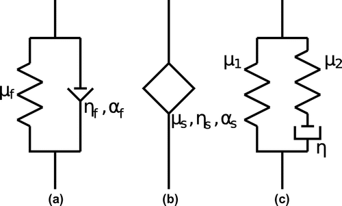
In this paper, we aim to develop a stable complex partial differential equation, p.d.e., solver to reconstruct the complex shear modulus from individual frequency content of the Fourier Transform of a single component of displacement data. We will test our algorithm on synthetically generated data for three viscoelastic models. Furthermore, we will utilize laboratory measured data from a gelatin phantom and fit the resulting frequency dependence to three different viscoelastic models: (1) the Kelvin–Voigt fractional derivative (KVFD) model [28,32–34]; (2) the Spring-pot (SP) model [31,32]; and (3) the Standard Linear Solid (SLS) model, also called the Zener model [35]. The diagrams of these three viscoelastic models are given in Figure 1.

The KVFD model and the SP model were established by the introduction of fractional calculus into the field of viscoelasticity, where a time dependence $t^{-\mathit{\alpha }}$ is added in the stress relaxation function. These models do not have finite propagation speed. However, in the frequencies represented in elastography experiments, it is possible to select parameters so that a good fit to the data can be obtained. Our third model, the Standard Linear Solid (SLS) model is causal; that is, it has finite propagation speed. It features an exponential time dependence in the stress relaxation pattern. Compared with the simple Voigt model and Maxwell model, the three viscoelastic models that we select in this paper have been shown to provide a better match over a wide range of frequencies when comparison is made with the viscoelastic response of tissue in prostate [28], brain [31] and liver [34]. Note that we will only include the viscoelastic effect for the deviatoric part of the stress–strain relationship because this is enough to provide a good data match.

Our equation systems for the three viscoelastic models in a plane strain model in 2D or in 3D are then:$$\begin{array}{cc}\text{KVFD}:\hfill & {\displaystyle \mathit{\rho }{\overrightarrow{u}}_{tt}=\mathrm{\nabla }(\mathit{\lambda }\mathrm{\nabla }·\overrightarrow{u})+\mathrm{\nabla }·\left[{\mathit{\mu }}_f\mathit{ϵ}+\frac{2{\mathit{\eta }}_f}{\mathrm{\Gamma }(1-{\mathit{\alpha }}_f)}{\int }_0^t\frac{1}{{(t-s)}^{{\mathit{\alpha }}_f}}\frac{\mathit{\partial }}{\mathit{\partial }s}\mathit{ϵ}\mathrm{d}s\right]}\hfill \\ \hfill & \\ \text{SP}:\hfill & {\displaystyle \mathit{\rho }{\overrightarrow{u}}_{tt}=\mathrm{\nabla }(\mathit{\lambda }\mathrm{\nabla }·\overrightarrow{u})+\mathrm{\nabla }·\left[\frac{2{\mathit{\mu }}_s{\mathit{\tau }}_s^{{\mathit{\alpha }}_s}}{\mathrm{\Gamma }(1-{\mathit{\alpha }}_s)}{\int }_0^t\frac{1}{{(t-s)}^{{\mathit{\alpha }}_s}}\frac{\mathit{\partial }}{\mathit{\partial }s}\mathit{ϵ}\mathrm{d}s\right]}\hfill \\ \hfill & \\ \text{SLS}:\hfill & {\displaystyle \mathit{\rho }{\overrightarrow{u}}_{tt}=\mathrm{\nabla }(\mathit{\lambda }\mathrm{\nabla }·\overrightarrow{u})+\mathrm{\nabla }·\left[2{\mathit{\mu }}_1\mathit{ϵ}+2{\int }_0^t{e}^{-(t-s)/\mathit{\tau }}\frac{\mathit{\partial }}{\mathit{\partial }s}({\mathit{\mu }}_2\mathit{ϵ})\mathrm{d}s\right],}\hfill \end{array}$$

where $\overrightarrow{u}$ is the displacement vector, $\mathit{ϵ}=\frac{1}{2}(\mathrm{\nabla }\overrightarrow{u}+{(\mathrm{\nabla }\overrightarrow{u})}^T)$ is the strain matrix, ${\mathit{\mu }}_f$ is the shear modulus in the Kelvin–Voigt fractional derivative model, ${\mathit{\mu }}_s$ is the shear modulus in the Spring-pot model and ${\mathit{\mu }}_1$ and ${\mathit{\mu }}_2$ are the shear moduli in the Standard Linear Solid Model; ${\mathit{\tau }}_s={\mathit{\eta }}_s/{\mathit{\mu }}_s$ is the relaxation time for the Spring-pot model and $\mathit{\tau }=\mathit{\eta }/{\mathit{\mu }}_2$ is the relaxation time for the Maxwell element in the Standard Linear Solid model; ${\mathit{\eta }}_f$ and $\mathit{\eta }$ are viscosities. The experiments under consideration are designed to have most of the information concentrated in one component [31,36] and we obtain data in only one image plane and for only one component, designated as u; furthermore, we assume we are in 2D and make a simplification. We use the corresponding viscoelastic wave equation models for the measured component:(1) $$\begin{array}{c}\hfill \mathit{\rho }{u}_{tt}=\mathrm{\nabla }·\left[{\mathit{\mu }}_f\mathrm{\nabla }u+\frac{{\mathit{\eta }}_f}{\mathrm{\Gamma }(1-{\mathit{\alpha }}_f)}{\int }_0^t\frac{1}{{(t-s)}^{{\mathit{\alpha }}_f}}\frac{\mathit{\partial }}{\mathit{\partial }s}(\mathrm{\nabla }u)\mathrm{d}s\right]+f,\end{array}$$(1) (2) $$\begin{array}{c}\hfill \mathit{\rho }{u}_{tt}=\mathrm{\nabla }·\left[\frac{{\mathit{\mu }}_s{\mathit{\tau }}_s^{{\mathit{\alpha }}_s}}{\mathrm{\Gamma }(1-{\mathit{\alpha }}_s)}{\int }_0^t\frac{1}{{(t-s)}^{{\mathit{\alpha }}_s}}\frac{\mathit{\partial }}{\mathit{\partial }s}(\mathrm{\nabla }u)\mathrm{d}s\right]+f,\end{array}$$(2) (3) $$\begin{array}{c}\hfill \mathit{\rho }{u}_{tt}=\mathrm{\nabla }·\left[{\mathit{\mu }}_1\mathrm{\nabla }u+{\int }_0^t{e}^{-(t-s)/\mathit{\tau }}\frac{\mathit{\partial }}{\mathit{\partial }s}({\mathit{\mu }}_2\mathrm{\nabla }u)\mathrm{d}s\right]+f,\end{array}$$(3)

in $\mathrm{\Omega }\times (0,T)$, where all the shear moduli ${\mathit{\mu }}_f,{\mathit{\mu }}_s,{\mathit{\mu }}_1,{\mathit{\mu }}_2$, the viscosities ${\mathit{\eta }}_f$, $\mathit{\eta }$, the relaxation times ${\mathit{\tau }}_s$, $\mathit{\tau }$ and the density $\mathit{\rho }$ are continuously differentiable. Note that this model can also be achieved by assuming that: (1) the tissue is nearly incompressible so that the volumetric change $\mathrm{\nabla }·u$ is small enough to be neglected; and (2) the compression wave is small enough and slowly varying enough that its contribution can be treated as noise; this would enable the term $\mathrm{\nabla }(\mathit{\lambda }\mathrm{\nabla }·u)$ to be treated as noise in the data. Here, we have also included the force, f, which represents the push used in the Acoustic Radiation force Crawling wave (ARC) experiment (see Section 4 for details). In the numerical experiments, this force is derived from the acoustic fields simulated using Field II ([37,38]). This push is described in more detail in Section 4. For the forward problem, the medium is initially at rest:(4) $$\begin{array}{c}\hfill u(x,y,0)=u_t(x,y,0)=0\text{on}\mathrm{\Omega }.\end{array}$$(4)

For the inverse problem model, since the data is movies of the displacement u throughout the 2D imaging region, we assume u(x, y, t) is given throughout $\mathrm{\Omega }$ and for an interval, $0<t\le T$, in time. Then, we: (1) change some of the targeted parameters in the inverse problem to be the ratio between the shear moduli and density or the ratios between the viscosities and density, by making the commonly accepted assumption that $\mathit{\rho }(x,y)$ is a constant; and (2) extract individual frequency content of the measured data by Fourier Transforming the forward Equations (1(1) $$\begin{array}{c}\hfill \mathit{\rho }{u}_{tt}=\mathrm{\nabla }·\left[{\mathit{\mu }}_f\mathrm{\nabla }u+\frac{{\mathit{\eta }}_f}{\mathrm{\Gamma }(1-{\mathit{\alpha }}_f)}{\int }_0^t\frac{1}{{(t-s)}^{{\mathit{\alpha }}_f}}\frac{\mathit{\partial }}{\mathit{\partial }s}(\mathrm{\nabla }u)\mathrm{d}s\right]+f,\end{array}$$(1) )–(3(3) $$\begin{array}{c}\hfill \mathit{\rho }{u}_{tt}=\mathrm{\nabla }·\left[{\mathit{\mu }}_1\mathrm{\nabla }u+{\int }_0^t{e}^{-(t-s)/\mathit{\tau }}\frac{\mathit{\partial }}{\mathit{\partial }s}({\mathit{\mu }}_2\mathrm{\nabla }u)\mathrm{d}s\right]+f,\end{array}$$(3) ) to the frequency domain:$$\left.\begin{array}{cc}{\displaystyle \mathrm{\nabla }·\left[{\mathit{\mu }}_f\mathrm{\nabla }u+\frac{{\mathit{\eta }}_f}{\mathrm{\Gamma }(1-{\mathit{\alpha }}_f)}{\int }_0^t\frac{1}{{(t-s)}^{{\mathit{\alpha }}_f}}\frac{\mathit{\partial }}{\mathit{\partial }s}(\mathrm{\nabla }u)\mathrm{d}s\right]-\mathit{\rho }{u}_{tt}=0}& \\ & \\ {\displaystyle \mathrm{\nabla }·\left[\frac{{\mathit{\mu }}_s{\mathit{\tau }}_s^{{\mathit{\alpha }}_s}}{\mathrm{\Gamma }(1-{\mathit{\alpha }}_s)}{\int }_0^t\frac{1}{{(t-s)}^{{\mathit{\alpha }}_s}}\frac{\mathit{\partial }}{\mathit{\partial }s}(\mathrm{\nabla }u)\mathrm{d}s\right]-\mathit{\rho }{u}_{tt}=0}& \\ & \\ {\displaystyle \mathrm{\nabla }·\left[{\mathit{\mu }}_1\mathrm{\nabla }u+{\int }_0^t{e}^{-(t-s)/\mathit{\tau }}\frac{\mathit{\partial }}{\mathit{\partial }s}({\mathit{\mu }}_2\mathrm{\nabla }u)\mathrm{d}s\right]-\mathit{\rho }{u}_{tt}=0}& \\ & \\ {\displaystyle \widehat{u}(x,y,\mathit{\omega })=\frac{1}{\sqrt{2\mathit{\pi }}}{\int }_{-\infty }^{+\infty }{e}^{-i\mathit{\omega }t}u(x,y,t)\mathrm{d}t}\end{array}\right\}⟹$$(5) $$\begin{array}{c}\hfill \mathrm{\nabla }\tilde{\mathit{\mu }}(x,y)·\mathrm{\nabla }\widehat{u}(x,y,{\mathit{\omega }}_c)+\tilde{\mathit{\mu }}(x,y)▵\widehat{u}(x,y,{\mathit{\omega }}_c)+{\mathit{\omega }}_c^2\widehat{u}(x,y,{\mathit{\omega }}_c)=0,\end{array}$$(5)

where$$\begin{array}{cc}\text{KVFD}:\hfill & {\displaystyle \tilde{\mathit{\mu }}=\left({\mathit{\mu }}_f+{\mathit{\eta }}_f{(i\mathit{\omega })}^{{\mathit{\alpha }}_f}\right)/\mathit{\rho }}\hfill \\ \hfill & \\ \text{SP}:\hfill & {\displaystyle \tilde{\mathit{\mu }}={\mathit{\mu }}_s{(i\mathit{\omega }{\mathit{\tau }}_s)}^{{\mathit{\alpha }}_s}/\mathit{\rho }}\hfill \\ \hfill & \\ \text{SLS}:\hfill & {\displaystyle \tilde{\mathit{\mu }}=\left({\mathit{\mu }}_1+\frac{{\mathit{\mu }}_{2}i\mathit{\omega }\mathit{\tau }}{i\mathit{\omega }\mathit{\tau }+1}\right)/\mathit{\rho }.}\hfill \end{array}$$

It is then, a complex shear modulus that needs to be recovered as a solution to (5(5) $$\begin{array}{c}\hfill \mathrm{\nabla }\tilde{\mathit{\mu }}(x,y)·\mathrm{\nabla }\widehat{u}(x,y,{\mathit{\omega }}_c)+\tilde{\mathit{\mu }}(x,y)▵\widehat{u}(x,y,{\mathit{\omega }}_c)+{\mathit{\omega }}_c^2\widehat{u}(x,y,{\mathit{\omega }}_c)=0,\end{array}$$(5) ) in the inverse problem. In the inverse problem, notice that the force term, f, has been eliminated as the source term will be located outside the imaging region.

As an often employed practice in the inverse problem of elastography, a simple Algebraic Inversion model can be achieved by making the locally constant assumption on $\tilde{\mathit{\mu }}$ and neglecting the first derivative terms of $\tilde{\mathit{\mu }}$ from (5(5) $$\begin{array}{c}\hfill \mathrm{\nabla }\tilde{\mathit{\mu }}(x,y)·\mathrm{\nabla }\widehat{u}(x,y,{\mathit{\omega }}_c)+\tilde{\mathit{\mu }}(x,y)▵\widehat{u}(x,y,{\mathit{\omega }}_c)+{\mathit{\omega }}_c^2\widehat{u}(x,y,{\mathit{\omega }}_c)=0,\end{array}$$(5) ):(6) $$\begin{array}{c}\hfill \widehat{\mathit{\mu }}(x,y)▵\widehat{u}(x,y,{\mathit{\omega }}_c))+{\mathit{\omega }}_c^2\widehat{u}(x,y,{\mathit{\omega }}_c))=0,\end{array}$$(6)

where we denote the approximated $\tilde{\mathit{\mu }}$ by $\widehat{\mathit{\mu }}$. Under some hypotheses, $\widehat{\mathit{\mu }}$ is a good approximation to $\tilde{\mathit{\mu }}$; see [39] for a rigorously established bound on the relative difference. However, when there are a number of high contrast inclusions in the viscoelastic background, solving the first-order partial differential Equation (5(5) $$\begin{array}{c}\hfill \mathrm{\nabla }\tilde{\mathit{\mu }}(x,y)·\mathrm{\nabla }\widehat{u}(x,y,{\mathit{\omega }}_c)+\tilde{\mathit{\mu }}(x,y)▵\widehat{u}(x,y,{\mathit{\omega }}_c)+{\mathit{\omega }}_c^2\widehat{u}(x,y,{\mathit{\omega }}_c)=0,\end{array}$$(5) ) can yield a more reliable estimation of shear viscoelasticity.

This paper then considers the reconstruction of a complex shear modulus $\tilde{\mathit{\mu }}$ by solving the first-order p.d.e.: that is, find complex valued $\tilde{\mathit{\mu }}$ by solving the complex differential equation(7) $$\begin{array}{c}\hfill \mathrm{\nabla }\tilde{\mathit{\mu }}(x,y)·\mathrm{\nabla }\widehat{u}(x,y,{\mathit{\omega }}_c)+\tilde{\mathit{\mu }}(x,y)▵\widehat{u}(x,y,{\mathit{\omega }}_c)+{\mathit{\omega }}_c^2\widehat{u}(x,y,{\mathit{\omega }}_c)=0.\end{array}$$(7)

Compared with the previous development of p.d.e. solvers for recovering the real shear modulus [40], the task here of recovering a complex shear modulus $\tilde{\mathit{\mu }}$ from the complex first-order p.d.e. (7(7) $$\begin{array}{c}\hfill \mathrm{\nabla }\tilde{\mathit{\mu }}(x,y)·\mathrm{\nabla }\widehat{u}(x,y,{\mathit{\omega }}_c)+\tilde{\mathit{\mu }}(x,y)▵\widehat{u}(x,y,{\mathit{\omega }}_c)+{\mathit{\omega }}_c^2\widehat{u}(x,y,{\mathit{\omega }}_c)=0.\end{array}$$(7) ) presents additional difficulty. The equation itself is non-hyperbolic and the exact solution of a non-hyperbolic system will exponentially grow with part of its growth rate determined by the imaginary part of the complex coefficients of the first-order derivative terms of $\tilde{\mathit{\mu }}$ [41,42]. In addition, even if we assume the complex shear modulus possesses no variation in one spatial dimension and reduce the first-order p.d.e. to an ordinary differential equation, the numerical error of the equation can still be exponentially growing with its growth rate determined by the real part of the complex coefficient of the zero-order derivative term of $\tilde{\mathit{\mu }}$, [42]. It has been shown that simple upwind discretization will fail and even a more advanced version of an upwind scheme is not stable for a non-hyperbolic system [41].

In this work, even though our equation is not hyperbolic, we propose a linear finite difference-based marching scheme to reconstruct $\tilde{\mathit{\mu }}$ by solving the inverse problem model as an evolution type of p.d.e. To control error growth, we use a combination of carefully selected multiple displacement data-sets. The numerical instability resulting from the complex coefficients of the first-order derivative terms of $\tilde{\mathit{\mu }}$ is controlled by a complex implicit upwind discretization and a modified Tikhonov regularization. The remaining error growth due to the coefficient of the zero-order derivative term of $\tilde{\mathit{\mu }}$ can be eliminated by combining multiple data-sets in a novel way. The proposed scheme, where only one first-order p.d.e. is solved but the coefficients are obtained using two data-sets, captures the spatial variation of the real and imaginary parts of the exact solution successfully. Note that this is not an iterative method as e.g. [43]. It has the potential of being faster than an iterative method (see [44] for a review of methods). We present the numerical method, the reconstruction of the complex shear modulus from simulated viscoelastic wave propagation data obtained from three viscoelastic models for the cases where we have two data-sets. Note that in all cases the numerical method exhibits stability but the performance can differ as we will show. We also compare the images, obtained with our algorithm, with Algebraic Inversion and show significant improvement. In addition, we add noise to the data and show the effect on the images.

Furthermore, we apply this algorithm to data-sets obtained at the Center for Biomedical Ultrasound at the University of Rochester. The experimental data is created with the new Acoustic Radiation Crawling (ARC) wave experiment performed on a gel phantom with an inclusion. For the laboratory data, we utilize the frequency content from eight frequencies and provide parameter choices determined by an $L^2$ optimization best fit for each of the viscoelastic models. Finally, for the laboratory data, we compare the complex modulus recoveries with the interference pattern phase wave speed recoveries.

The structure of this paper is as follows: In Section 2, we present finite difference discretization of the numerical scheme and the modified Tikhonov regularization. We exhibit better results when we use multiple data-sets. In Section 3, we describe the viscoelastic wave equation simulation and give the numerical reconstruction of the complex shear modulus from synthetic data including results when we add noise to the synthetic data. In Section 4, the experiment is described. Section 5 is devoted to the complex shear modulus recovery from phantom data and the matching of frequency dependence to our three viscoelastic models. In Section 6, we give a comparison of the complex modulus recovery with the phase wave speed recovery. We do this since we have previously presented phase wave speed recoveries from interference patterns. Finally, we conclude this document and give ideas on future work.

2. Linear explicit-implicit upwind scheme

The first-order complex equation we use for the recovery of the complex shear modulus $\tilde{\mathit{\mu }}$ for individual frequency content can be changed to an evolution type of p.d.e. in the following way assuming the x direction is a pseudo-time direction and ${\widehat{u}}_x\ne 0$:(8) $$\begin{array}{c}\hfill {\tilde{\mathit{\mu }}}_x{\widehat{u}}_x+{\tilde{\mathit{\mu }}}_y{\widehat{u}}_y+\tilde{\mathit{\mu }}▵\widehat{u}=-{\mathit{\omega }}^2\widehat{u}⟹{\tilde{\mathit{\mu }}}_x+a{\tilde{\mathit{\mu }}}_y+b\tilde{\mathit{\mu }}=c,\end{array}$$(8)

where $a={\widehat{u}}_y{({\widehat{u}}_x)}^{-1},b=▵\widehat{u}{({\widehat{u}}_x)}^{-1},c=-{\mathit{\omega }}^2\widehat{u}{({\widehat{u}}_x)}^{-1}$ are all complex functions. We can discretize the equation above with the following finite difference scheme where we assume uniform discretization in y and denote the solution of the discretized problem on the grid as ${\widetilde{\stackrel{~}{\mathit{\mu }}}}_{i,j},1\le i\le M,1\le j\le N$:$${\displaystyle \frac{{\widetilde{\stackrel{~}{\mathit{\mu }}}}_{i+1,j}-{\widetilde{\stackrel{~}{\mathit{\mu }}}}_{i,j}}{\mathrm{d}{x}_i}+a_{i,j}\left\{\begin{array}{cc}{\displaystyle \frac{{\widetilde{\stackrel{~}{\mathit{\mu }}}}_{i+1,j+1}-{\widetilde{\stackrel{~}{\mathit{\mu }}}}_{i+1,j}}{\mathrm{d}y}}\hfill & {\displaystyle Re(a_{i,j})<0}\hfill \\ \hfill & \\ {\displaystyle \frac{{\widetilde{\stackrel{~}{\mathit{\mu }}}}_{i+1,j}-{\widetilde{\stackrel{~}{\mathit{\mu }}}}_{i+1,j-1}}{\mathrm{d}y}}\hfill & {\displaystyle Re(a_{i,j})\ge 0}\hfill \end{array}\right.+b_{i,j}{\widetilde{\stackrel{~}{\mathit{\mu }}}}_{i,j}=c_{i,j}.}$$

where $\mathrm{d}{x}_i$ is the variable pseudo time step size. This explicit-implicit scheme can be rewritten as:(9) $$\begin{array}{c}\hfill A_i{\overrightarrow{\widetilde{\stackrel{~}{\mathit{\mu }}}}}_{i+1}={\overrightarrow{c}}_i\mathrm{d}{x}_i+B_i{\overrightarrow{\widetilde{\stackrel{~}{\mathit{\mu }}}}}_i,\end{array}$$(9)

where $A_i=(A_{i:k,l}),1\le k\le n,1\le l\le n$ is a tridiagonal matrix with its nonzero entries defined by the following formulas:(10) $$\begin{array}{c}\hfill A_{i:k,k}=1+sign(Re(a_{i,k}))a_{i,k}\frac{\mathrm{d}{x}_i}{\mathrm{d}y},\\ \hfill A_{i:k,k+1}=\frac{-sign(Re(a_{i,k}))+1}{2}{a}_{i,k}\frac{\mathrm{d}{x}_i}{\mathrm{d}y},\\ \hfill A_{i:k,k-1}=\frac{-sign(Re(a_{i,k}))-1}{2}{a}_{i,k}\frac{\mathrm{d}{x}_i}{\mathrm{d}y},\end{array}$$(10)

and $B_i$ is a diagonal matrix whose entries are defined by ${(B_i)}_{k,k}=1-b_{i,k}\mathrm{d}{x}_i$. Notice that $|A_{i:k,k}|\ge 1$ and for every pair of $A_{i:k,k+1}$ and $A_{i:k,k-1}$, there is only one of them that is nonzero. The stability and accuracy of the matrix inversion is determined by the norm of the inverse of $A_i$, i.e. the eigenvalues of ${\overline{A}}_i^T{A}_i$. Now let $({\mathit{\xi }}_j^i,{\overrightarrow{\mathit{\eta }}}_j^i)$ be the eigenvalue and eigenvector pairs of ${\overline{A}}_i^T{A}_i$ and let $0<{\mathit{\xi }}_1^i\le {\mathit{\xi }}_2^i\le \cdots \le {\mathit{\xi }}_n^i$. If ${\mathit{\xi }}_1^i\ge 1$, then we solve (9(9) $$\begin{array}{c}\hfill A_i{\overrightarrow{\widetilde{\stackrel{~}{\mathit{\mu }}}}}_{i+1}={\overrightarrow{c}}_i\mathrm{d}{x}_i+B_i{\overrightarrow{\widetilde{\stackrel{~}{\mathit{\mu }}}}}_i,\end{array}$$(9) ) by direct matrix inversion. Now suppose $0<{\mathit{\xi }}_1^i\le 1$, we solve the following equation instead:(11) $$\begin{array}{c}\hfill A_i{\overrightarrow{\widetilde{\stackrel{~}{\mathit{\mu }}}}}_{i+1}=\sqrt{{\mathit{\xi }}_1^i}\left({\overrightarrow{c}}_i\mathrm{d}{x}_i+B_i{\overrightarrow{\widetilde{\stackrel{~}{\mathit{\mu }}}}}_i\right)=min(1,\sqrt{{\mathit{\xi }}_1^i})\left({\overrightarrow{c}}_i\mathrm{d}{x}_i+B_i{\overrightarrow{\widetilde{\stackrel{~}{\mathit{\mu }}}}}_i\right).\end{array}$$(11)

This is equivalent to Tikhonov regularization on the matrix inversion, i.e. finding the optimal diagonal matrix $D_i$ s.t.$$\Vert {(D+{\overline{A}}_i^T{A}_i)}^{-1}{\overline{A}}_i^T{\Vert }_2\le 1.$$

To stabilize the matrix inversion, we consider Tikhonov regularization in $l_2$ norm.

Lemma 2.1:

There exists a diagonal matrix $D_i$ for each $A_i$, s.t.$$\Vert {\overrightarrow{\widetilde{\stackrel{~}{\mathit{\mu }}}}}_{i+1}{\Vert }_2\le {\Vert {\overrightarrow{g}}_i\Vert }_2\text{for}(D+{\overline{A}}_i^T{A}_i){\overrightarrow{\widetilde{\stackrel{~}{\mathit{\mu }}}}}_{i+1}={\overline{A}}_i^T{\overrightarrow{g}}_i.$$

Proof Consider the matrix inversion as a $L^2$ minimization problem. That is, to find ${\overrightarrow{\widetilde{\stackrel{~}{\mathit{\mu }}}}}_{i+1}$ such that$$\underset{{\overrightarrow{\widetilde{\stackrel{~}{\mathit{\mu }}}}}_i\in {\mathbb{C}}^n}{min}{\Vert A_i{\overrightarrow{\widetilde{\stackrel{~}{\mathit{\mu }}}}}_{i+1}-{\overrightarrow{c}}_i\mathrm{d}{x}_i-B_i{\overrightarrow{\widetilde{\stackrel{~}{\mathit{\mu }}}}}_i\Vert }_2^2=\underset{{\overrightarrow{\widetilde{\stackrel{~}{\mathit{\mu }}}}}_i\in {\mathbb{C}}^n}{min}I({\overrightarrow{\widetilde{\stackrel{~}{\mathit{\mu }}}}}_i).$$

Assume ${\overrightarrow{\widetilde{\stackrel{~}{\mathit{\mu }}}}}_i$ as known and let ${\overrightarrow{g}}_i={\overrightarrow{c}}_i\mathrm{d}{x}_i+B_i{\overrightarrow{\widetilde{\stackrel{~}{\mathit{\mu }}}}}_i$. Then the minimization problem ${min}_{{\overrightarrow{\widetilde{\stackrel{~}{\mathit{\mu }}}}}_i\in {\mathbb{C}}^n}I({\overrightarrow{\widetilde{\stackrel{~}{\mathit{\mu }}}}}_i)$ becomes$$\underset{{\overrightarrow{\widetilde{\stackrel{~}{\mathit{\mu }}}}}_i\in {\mathbb{C}}^n}{min}{\Vert A_i{\overrightarrow{\widetilde{\stackrel{~}{\mathit{\mu }}}}}_{i+1}-{\overrightarrow{g}}_i\Vert }_2^2.$$

To minimize, we need to solve for(12) $$\begin{array}{c}\hfill ({\overline{A}}_i^T{A}_i){\overrightarrow{\widetilde{\stackrel{~}{\mathit{\mu }}}}}_{i+1}={\overline{A}}_i^T{\overrightarrow{g}}_i.\end{array}$$(12)

Now let $({\mathit{\xi }}_j^i,{\overrightarrow{\mathit{\eta }}}_j^i)$ be the eigenvalue and eigenvector pair of ${\overline{A}}_i^T{A}_i$ and let $0<{\mathit{\xi }}_1^i\le {\mathit{\xi }}_2^i\le \cdots \le {\mathit{\xi }}_n^i$. If ${\mathit{\xi }}_1^i\ge 1$, then we can solve for$${\overrightarrow{\widetilde{\stackrel{~}{\mathit{\mu }}}}}_{i+1}=A_i^{-1}{\overrightarrow{g}}_i\text{and}\Vert {\overrightarrow{\widetilde{\stackrel{~}{\mathit{\mu }}}}}_{i+1}{\Vert }_2\le {\Vert {\overrightarrow{g}}_i\Vert }_2.$$

Now suppose $0<{\mathit{\xi }}_1^i\le 1$, we can change the minimization problem by representing ${\overrightarrow{\widetilde{\stackrel{~}{\mathit{\mu }}}}}_{i+1}={\sum }_{i=1}^n({\overrightarrow{\widetilde{\stackrel{~}{\mathit{\mu }}}}}_{i+1},{\overrightarrow{\mathit{\eta }}}_j^i){\overrightarrow{\mathit{\eta }}}_j^i$ and get$$\begin{array}{cc}& {\displaystyle \underset{{\overrightarrow{\widetilde{\stackrel{~}{\mathit{\mu }}}}}_{i+1}\in {\mathbb{C}}^n}{min}\left[\Vert D{\overrightarrow{\widetilde{\stackrel{~}{\mathit{\mu }}}}}_{i+1}{\Vert }_2^2+{\Vert A_i{\overrightarrow{\widetilde{\stackrel{~}{\mathit{\mu }}}}}_{i+1}-{\overrightarrow{g}}_i\Vert }_2^2\right]}\hfill \\ \hfill & {\displaystyle =\underset{{\overrightarrow{\widetilde{\stackrel{~}{\mathit{\mu }}}}}_{i+1}\in {\mathbb{C}}^n}{min}\left[{∥\sum _{i=1}^n\sqrt{d_j}({\overrightarrow{\widetilde{\stackrel{~}{\mathit{\mu }}}}}_{i+1},{\overrightarrow{\mathit{\eta }}}_j^i){\overrightarrow{\mathit{\eta }}}_j^i∥}_2^2+{\Vert A_i{\overrightarrow{\widetilde{\stackrel{~}{\mathit{\mu }}}}}_{i+1}-{\overrightarrow{g}}_i\Vert }_2^2\right]}\hfill \\ \hfill & {\displaystyle =\underset{{\overrightarrow{\widetilde{\stackrel{~}{\mathit{\mu }}}}}_{i+1}\in {\mathbb{C}}^n}{min}{I}_{\mathit{\alpha }}({\overrightarrow{\widetilde{\stackrel{~}{\mathit{\mu }}}}}_{i+1}),\text{where}\mathit{\alpha }>0,}\hfill \end{array}$$

where D is a diagonal matrix with diagonal element $d_j>0$. In this case, we have(13) $$\begin{array}{c}\hfill (D+{\overline{A}}_i^T{A}_i){\overrightarrow{\widetilde{\stackrel{~}{\mathit{\mu }}}}}_{i+1}={\overline{A}}_i^T{\overrightarrow{g}}_i,\end{array}$$(13)

which is equivalent to$${\overrightarrow{\widetilde{\stackrel{~}{\mathit{\mu }}}}}_{i+1}=\sum _{j=1}^n\left(\frac{{\mathit{\xi }}_j^i}{d_j+{\mathit{\xi }}_j^i}\right)(A^{-1}{\overrightarrow{g}}_i,{\overrightarrow{\mathit{\eta }}}_j^i){\overrightarrow{\mathit{\eta }}}_j^i\Rightarrow$$$$\begin{array}{cc}{\displaystyle \Vert {\overrightarrow{\widetilde{\stackrel{~}{\mathit{\mu }}}}}_{i+1}{\Vert }_2^2}\hfill & {\displaystyle ={\sum }_{j=1}^n{\left(\frac{{\mathit{\xi }}_j^i}{d_j+{\mathit{\xi }}_j^i}\right)}^2{\left|(A^{-1}{\overrightarrow{g}}_i,{\overrightarrow{\mathit{\eta }}}_j^i){\overrightarrow{\mathit{\eta }}}_j^i\right|}^2}\hfill \\ \hfill & \hfill & \\ \hfill & {\displaystyle \le {\left[{max}_j\left(\frac{{\mathit{\xi }}_j^i}{d_j+{\mathit{\xi }}_j^i}\right)\right]}^2{\Vert A^{-1}{\overrightarrow{g}}_i\Vert }_2^2.}\hfill \end{array}$$

Since $\Vert A^{-1}{\Vert }_2=\frac{1}{\sqrt{{\mathit{\xi }}_1^i}}$, if we choose $d_j={\mathit{\xi }}_j^i\left[{\left({\mathit{\xi }}_1^i\right)}^{-1/2}-1\right]$, we will have$$\frac{{\mathit{\xi }}_j^i}{(d_j+{\mathit{\xi }}_j^i)\sqrt{{\mathit{\xi }}_1^i}}=1\Rightarrow \Vert {\overrightarrow{\widetilde{\stackrel{~}{\mathit{\mu }}}}}_{i+1}{\Vert }_2\le {\Vert {\overrightarrow{g}}_i\Vert }_2.$$

The structure of the matrix $A^i$ ensures row diagonal dominance:$$\begin{array}{cc}{\displaystyle |A_{k,k}^i|}\hfill & {\displaystyle =\sqrt{{\left(1+|Re(a_{i,k})|\frac{\mathrm{d}{x}_i}{\mathrm{d}y}\right)}^2+{\left(|Im(a_{i,k})|\frac{\mathrm{d}{x}_i}{\mathrm{d}y}\right)}^2}}\hfill \\ \hfill & \hfill & \\ \hfill & {\displaystyle >{\sum }_{l\ne k}|A_{k,l}^i|=\sqrt{{\left(|Re(a_{i,k})|\frac{\mathrm{d}{x}_i}{\mathrm{d}y}\right)}^2+{\left(|Im(a_{i,k})|\frac{\mathrm{d}{x}_i}{\mathrm{d}y}\right)}^2}=|a_{i,k}|\frac{\mathrm{d}{x}_i}{\mathrm{d}y}}\hfill \end{array}$$

3. Numerical analysis

3.1. Stability

We first present the stability analysis of the linear explicit-implicit hyperbolic scheme and then the fractional-order convergence result will follow with the regularization term. Consider the homogeneous part of (8(8) $$\begin{array}{c}\hfill {\tilde{\mathit{\mu }}}_x{\widehat{u}}_x+{\tilde{\mathit{\mu }}}_y{\widehat{u}}_y+\tilde{\mathit{\mu }}▵\widehat{u}=-{\mathit{\omega }}^2\widehat{u}⟹{\tilde{\mathit{\mu }}}_x+a{\tilde{\mathit{\mu }}}_y+b\tilde{\mathit{\mu }}=c,\end{array}$$(8) ). We assume $\tilde{\mathit{\mu }}\in {\mathbb{C}}^2(R)$ satisfies:(14) $$\begin{array}{c}\hfill {\tilde{\mathit{\mu }}}_x+a(x,y){\tilde{\mathit{\mu }}}_y+b(x,y)\tilde{\mathit{\mu }}=0,\end{array}$$(14)

where the domain $R=\{(x,y)|0\le x\le L,0\le y\le L^{\ast }\}$ and $a,b\in \mathbb{C}(R)$. Let ${\overrightarrow{\widetilde{\stackrel{~}{\mathit{\mu }}}}}_i$ be the numerical solution at the ith step $x_i$. We first seek stability results where we show there exists $C,\widehat{C}>0$ with $\Vert {\overrightarrow{\widetilde{\stackrel{~}{\mathit{\mu }}}}}_{i+1}{\Vert }_2\le C{\Vert {\overrightarrow{\widetilde{\stackrel{~}{\mathit{\mu }}}}}_i\Vert }_2$ so that independent of step size, at the final nth step $\Vert {\overrightarrow{\widetilde{\stackrel{~}{\mathit{\mu }}}}}_n{\Vert }_2\le \widehat{C}{\Vert {\overrightarrow{\widetilde{\stackrel{~}{\mathit{\mu }}}}}_0\Vert }_2$. Nevertheless, the constant C can be large. We improve on the constant later in the paper by utilizing optimal data-sets.

Lemma 3.1:

There exists $\mathit{\alpha }$ independent of step sizes such that$$\Vert {\overrightarrow{\widetilde{\stackrel{~}{\mathit{\mu }}}}}_{i+1}{\Vert }_2\le e^{\mathit{\alpha }\mathrm{d}{x}_i}{\Vert {\overrightarrow{\widetilde{\stackrel{~}{\mathit{\mu }}}}}_i\Vert }_2,$$

where $\mathit{\alpha }={max}_{i,j}|b_{i,j}|$. Furthermore $\Vert {\overrightarrow{\widetilde{\stackrel{~}{\mathit{\mu }}}}}_n{\Vert }_2\le e^{\mathit{\alpha }L}{\Vert {\overrightarrow{\widetilde{\stackrel{~}{\mathit{\mu }}}}}_0\Vert }_2$.

Proof If Equation (14(14) $$\begin{array}{c}\hfill {\tilde{\mathit{\mu }}}_x+a(x,y){\tilde{\mathit{\mu }}}_y+b(x,y)\tilde{\mathit{\mu }}=0,\end{array}$$(14) ) is solved by regularized numerical scheme (11(11) $$\begin{array}{c}\hfill A_i{\overrightarrow{\widetilde{\stackrel{~}{\mathit{\mu }}}}}_{i+1}=\sqrt{{\mathit{\xi }}_1^i}\left({\overrightarrow{c}}_i\mathrm{d}{x}_i+B_i{\overrightarrow{\widetilde{\stackrel{~}{\mathit{\mu }}}}}_i\right)=min(1,\sqrt{{\mathit{\xi }}_1^i})\left({\overrightarrow{c}}_i\mathrm{d}{x}_i+B_i{\overrightarrow{\widetilde{\stackrel{~}{\mathit{\mu }}}}}_i\right).\end{array}$$(11) ), we obtain:$$\Vert {\overrightarrow{\widetilde{\stackrel{~}{\mathit{\mu }}}}}_{i+1}{\Vert }_2\le \sqrt{{\mathit{\xi }}_1^i}|A_i^{-1}{\Vert }_2·\underset{j}{max}|1-b_{i,j}\mathrm{d}{x}_i|·\Vert {\overrightarrow{\widetilde{\stackrel{~}{\mathit{\mu }}}}}_i{\Vert }_2\le e^{\mathit{\alpha }\mathrm{d}{x}_i}{\Vert {\overrightarrow{\widetilde{\stackrel{~}{\mathit{\mu }}}}}_i\Vert }_2.$$

The second inequality follows directly.

This proves the stability of the linear numerical scheme in the $l^2$ norm (see (2.4.2) from [45]).

3.2. Error control with combination of multiple data-sets

To completely control the growth of the numerical solution, we invoke the concept of combining multiple displacement data-sets to eliminate the zero-order derivative term of $\tilde{\mathit{\mu }}$ from the first-order p.d.e. that governs the inverse problem solution.

Suppose we have two individual sets of displacement data, $u_j,j=1,2$, obtained from two separate experiments for the same medium, then both data-sets satisfy the same first-order equation in the inverse problem:$${\widehat{u}}_{j,x}{\tilde{\mathit{\mu }}}_x+{\widehat{u}}_{j,y}{\tilde{\mathit{\mu }}}_y+\tilde{\mathit{\mu }}▵{\widehat{u}}_j+{\mathit{\omega }}^2{\widehat{u}}_j=0,j=1,2.$$

By the following simple algebra step, we obtain:$$\left.\begin{array}{cc}▵{\widehat{u}}_2({\widehat{u}}_{1,x}{\tilde{\mathit{\mu }}}_x+{\widehat{u}}_{1,y}{\tilde{\mathit{\mu }}}_y+\tilde{\mathit{\mu }}▵{\widehat{u}}_1+{\mathit{\omega }}^2{\widehat{u}}_1)=0\hfill & \\ \hfill & \\ -▵{\widehat{u}}_1({\widehat{u}}_{2,x}{\tilde{\mathit{\mu }}}_x+{\widehat{u}}_{2,y}{\tilde{\mathit{\mu }}}_y+\tilde{\mathit{\mu }}▵{\widehat{u}}_2+{\mathit{\omega }}^2{\widehat{u}}_2)=0\hfill \end{array}\right\}⟹$$$$(▵{\widehat{u}}_2{\widehat{u}}_{1,x}-▵{\widehat{u}}_1{\widehat{u}}_{2,x}){\tilde{\mathit{\mu }}}_x+(▵{\widehat{u}}_2{\widehat{u}}_{1,y}-▵{\widehat{u}}_1{\widehat{u}}_{2,y}){\tilde{\mathit{\mu }}}_y=-{\mathit{\omega }}^2(▵{\widehat{u}}_2{\widehat{u}}_1-▵{\widehat{u}}_1{\widehat{u}}_2)⟹$$(15) $$\begin{array}{c}\hfill {\tilde{\mathit{\mu }}}_x+\tilde{a}{\tilde{\mathit{\mu }}}_y=\tilde{c},\end{array}$$(15)

where$$a=\frac{▵{\widehat{u}}_2{\widehat{u}}_{1,y}-▵{\widehat{u}}_1{\widehat{u}}_{2,y}}{(▵{\widehat{u}}_2{\widehat{u}}_{1,x}-▵{\widehat{u}}_1{\widehat{u}}_{2,x})},c=\frac{-{\mathit{\omega }}^2(▵{\widehat{u}}_2{\widehat{u}}_1-▵{\widehat{u}}_1{\widehat{u}}_2)}{(▵{\widehat{u}}_2{\widehat{u}}_{1,x}-▵{\widehat{u}}_1{\widehat{u}}_{2,x})}.$$

Equation (15(15) $$\begin{array}{c}\hfill {\tilde{\mathit{\mu }}}_x+\tilde{a}{\tilde{\mathit{\mu }}}_y=\tilde{c},\end{array}$$(15) ) is a simple transport equation with no zero-order derivative term of $\tilde{\mathit{\mu }}$ and if we use the same complex upwind discretization on the equation above, we will get:$$A^i{\overrightarrow{\widetilde{\stackrel{~}{\mathit{\mu }}}}}_{i+1}={\overrightarrow{\tilde{c}}}_i\mathrm{d}{x}_i+{\overrightarrow{\widetilde{\stackrel{~}{\mathit{\mu }}}}}_i.$$

In this case, the contribution of solution growth from the $b_{i,j}$ term is gone as the zero-order derivative term of $\tilde{\mathit{\mu }}$ is eliminated from the equation governing the solution of the inverse problem. Provided that $(▵{\widehat{u}}_2{\widehat{u}}_{1,x}-▵{\widehat{u}}_1{\widehat{u}}_{2,x})$ is bounded away from zero, the numerical scheme is stable and the constant $e^{\mathit{\alpha }L}$ in Lemma 3.1 is significantly reduced. Examples will be given in the next section to exhibit the superior stability control of this data combination.

4. Performance test on simulated data

In this section, we test the linear explicit-implicit hyperbolic scheme and compare its performance with the result obtained using the Algebraic Inversion Method.

The forward simulation has many similar features as that given in [36]: here, we solve the viscoelastic wave equations for all three viscoelastic models$$\begin{array}{cc}\text{KVFD}:\hfill & {\displaystyle \mathit{\rho }{u}_{tt}=\mathrm{\nabla }·\left[{\mathit{\mu }}_f\mathrm{\nabla }u+\frac{{\mathit{\eta }}_f}{\mathrm{\Gamma }(1-{\mathit{\alpha }}_f)}{\int }_0^t\frac{1}{{(t-s)}^{{\mathit{\alpha }}_f}}\frac{\mathit{\partial }}{\mathit{\partial }s}(\mathrm{\nabla }u)\mathrm{d}s\right]+f,}\hfill \\ \hfill & \\ \text{SP}:\hfill & {\displaystyle \mathit{\rho }{u}_{tt}=\mathrm{\nabla }·\left[\frac{{\mathit{\mu }}_s{\mathit{\tau }}_s^{{\mathit{\alpha }}_s}}{\mathrm{\Gamma }(1-{\mathit{\alpha }}_s)}{\int }_0^t\frac{1}{{(t-s)}^{{\mathit{\alpha }}_s}}\frac{\mathit{\partial }}{\mathit{\partial }s}(\mathrm{\nabla }u)\mathrm{d}s\right]+f,}\hfill \\ \hfill & \\ \text{SLS}:\hfill & {\displaystyle \mathit{\rho }{u}_{tt}=\mathrm{\nabla }·\left[{\mathit{\mu }}_1\mathrm{\nabla }u+{\int }_0^t{e}^{-(t-s)/\mathit{\tau }}\frac{\mathit{\partial }}{\mathit{\partial }s}({\mathit{\mu }}_2\mathrm{\nabla }u)\mathrm{d}s\right]+f.}\hfill \end{array}$$

In this study for our forward simulations, we allow all stiffness parameters (with the exception of ${\mathit{\alpha }}_f$, ${\mathit{\alpha }}_s$, and $\mathit{\tau }$) in the viscoelastic model to be spatially varying, which effectively provides spatial dependence for both the real and imaginary parts of the complex shear modulus $\tilde{\mathit{\mu }}$. The forcing function f for all three models is generated by Field II, a program for simulating ultrasound transducer fields and ultrasound imaging using linear acoustics. To simulate the acoustic radiation force used in the ARC experiment, we used the physical parameters of a specially built transrectal transducer as inputs to the Field II simulation. The pitch of the transducer array was 203 microns and the centre frequency was approximately 5 MHz. Using these parameters, a two-dimensional intensity function was calculated using Field II. The simulated intensity map is assumed to be proportional to the applied force, using the following equation ([46]):$$f=\frac{2\tilde{\mathit{\alpha }}I}{c}$$

where $\tilde{\mathit{\alpha }}$ is the absorption coefficient, I is the temporal average intensity, and c is the speed of sound in water. Using this relationship, the simulated intensities can be used to derive the force for a $250\mathrm{\mu }\mathrm{s}$ pushing pulse as used in the experiment (see Section 5 for more details about the experiment). We note that with this forcing function we do not compute the scattered field as in [36] and then add the scattered field and a closed form incident field. Here, we compute the total displacement directly.

We use a second-order finite difference scheme in time and space to discretize the displacement in the forward equation. We assume the Sommerfeld radiation condition for the wave and implement a second-order split-field perfectly matched layer absorbing boundary condition around the computational domain to prevent numerical reflections of outgoing waves (see [36,47]). To avoid numerical problems in the inverse problem, the so-called ‘inverse crime’, we use the synthetic data from the forward simulation on the forward problem computational grid to generate a new set of displacement data on a different grid. To do this for each time frame, we first make a two-dimensional cubic spline interpolation and then sample the interpolated displacement on a new mesh. The grid size of the new mesh is two-thirds of the grid size of the old mesh used in the forward simulation.

We Fourier Transform the data-set in time and extract content at each of several frequencies. In each case, to compute the numerical derivatives of the complex data, we first separate the phase and the amplitude as $\widehat{u}=M{e}^{i\mathit{\varphi }}$. The derivatives of $\widehat{u}$ are then calculated in terms of derivatives of M and $\mathit{\varphi }$ by an averaging method (see [48]) with a 3 by 3 window to eliminate numerical noise. To resolve the jump discontinuities in the wrapped phase $\mathit{\varphi }$, we utilize an $L^1$ minimization procedure (see [49]) to perform multidimensional phase unwrapping.

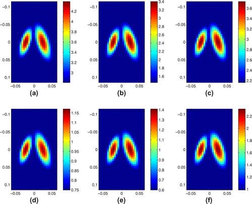
Figure 2. Exact value of complex modulus at frequency 25 Hz(KVFD), 20 Hz(SP) and 12.5 Hz(SLS): (a) real part, KVFD model; (b) real part, SP model; (c) real part, SLS model; (d) imaginary part, KVFD model; (e) imaginary part, SP model; (f) imaginary part, SLS model. Notice that in all cases, the imaginary part is smaller than the real part. The units for the images are KPa.

For the linear hyperbolic forward problem p.d.e. solver, we generate two sets of data from two different simulations: one with the Field II push on top of the domain and the other with the Field II generated push at the bottom of the domain. The time step size used during the simulation is 0.5 ms. These two individual data-sets and their numerical derivatives are used separately or together, as described in Section 3, and then fed to the linear p.d.e. solver. For the Algebraic Inversion method, we only use one of those two data-sets to compute numerical derivatives and the application of it is much more straightforward. The results given in this section are obtained from frequency contents at 20.80 Hz for the KVFD model, 16.65 Hz for the SP model and 19.13 Hz for the SLS model.

For all three viscoelastic models, the real and imaginary parts of the exact shear modulus have two elliptical inclusions in a constant background. The input parameters to the simulation are defined using the following procedure:$$\begin{array}{cc}g(x,y)\hfill & {\displaystyle =Amax\left(0.{0015}^2-\frac{{(xcos(2\mathit{\pi }/5)+(y+0.0025)sin(2\mathit{\pi }/5))}^2}{0.0025}\right.}\hfill \\ \hfill & \hfill & \\ \hfill & \hfill & {\displaystyle -\left.\frac{{(xsin(2\mathit{\pi }/5)-(y+0.0025)cos(2\mathit{\pi }/5))}^2}{0.02},0\right)}\hfill \\ \hfill & \hfill & \\ \hfill & \hfill & {\displaystyle +Bmax\left(0.{003}^2-\frac{{(xcos(-2\mathit{\pi }/5)+(y+0.0025)sin(-2\mathit{\pi }/5))}^2}{0.002}\right.}\hfill \\ \hfill & \hfill & \\ \hfill & \hfill & {\displaystyle -\left.\frac{{(xsin(-2\mathit{\pi }/5)-(y+0.0025)cos(-2\mathit{\pi }/5))}^2}{0.015},0\right)+{\mathit{\mu }}_0}\hfill \end{array}$$$$\begin{array}{cc}\text{KVFD}:\hfill & {\displaystyle {\mathit{\mu }}_f=g(x,y),{\mathit{\mu }}_0=1,{\mathit{\eta }}_f=0.5{\mathit{\mu }}_f,{\mathit{\alpha }}_f=0.25,A=0.25e+6,B=0.6e+5}\hfill \\ \hfill & \\ \text{SP}:\hfill & {\displaystyle {\mathit{\mu }}_s=g(x,y),{\mathit{\mu }}_0=2,{\mathit{\tau }}_s=0.002,{\mathit{\alpha }}_s=0.25,A=1.2e+6,B=0.3e+5}\hfill \\ \hfill & \\ \text{SLS}:\hfill & {\displaystyle {\mathit{\mu }}_1=1,{\mathit{\mu }}_2=g(x,y),{\mathit{\mu }}_0=2,\mathit{\tau }=0.01,A=1.2e+6,B=0.3e+6}\hfill \end{array}$$

We present numerical reconstruction results from three synthetic data-sets, two data-sets for each of the three viscoelastic models. In Figure 2, we show the true values of the real and imaginary parts of the modulus $\tilde{\mathit{\mu }}$ in the KVFD, SP and SLS models.

In Figure 3, we present reconstruction results that are computed from two data-sets for each model using Equation (15(15) $$\begin{array}{c}\hfill {\tilde{\mathit{\mu }}}_x+\tilde{a}{\tilde{\mathit{\mu }}}_y=\tilde{c},\end{array}$$(15) ). Note that the recoveries of the real and imaginary parts of the complex modulus captures the size and the location of the inclusion perfectly while undershoots the amplitude of the exact value. This is due to the regularization effect on the growth of the numerical solution. Lastly, the Algebraic Inversion results are presented in Figure 4. It is very clear that the Algebraic Inversion is much less reliable in recovering the complex shear modulus in this practical simulation set up.

Figure 3. Recovery from two data-sets: (a) real part, KVFD model; (b) real part, SP model; (c) real part, SLS model; (d) imaginary part, KVFD model; (e) imaginary part, SP model; (f) imaginary part, SLS model. The units for the images are KPa.

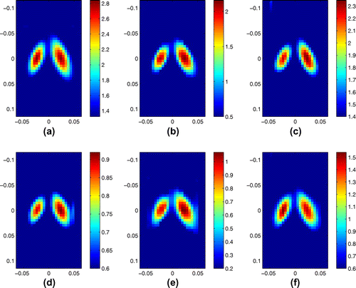
Figure 4. Recovery from algebraic inversion: (a) real part, KVFD model; (b) imaginary part, KVFD model; (c) absolute value of the error of real part, KVFD Model; (d) absolute value of the error of imaginary part, KVFD Model; (e) real part, SP Model; (f) imaginary part, SP model; (g) absolute value of the error of real part, SP model; (h) absolute value of the error of imaginary part, SP Model; (i) real part, SLS Model; (j) imaginary part, SLS model; (k) absolute value of the error of real part, SLS model; (l) absolute value of the error of imaginary part, SLS Model. The units for the images are KPa.

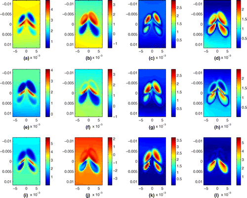
Finally, we present results from noisy synthetic data. We added $1\%$ Gaussian noise to the synthetic data and reconstructed the complex modulus using our regularized complex elastographic hyperbolic solver. In Figure 5, the recovery from two data-sets is demonstrated. Our numerical solver captures the location and the size of the inclusions but the amplitude is underestimated. Note that the imaginary part of the shear modulus degrades, with the addition of noise, more than the real part of the shear modulus.

Figure 5. Recovery from two data-sets: (a) real part, KVFD model; (b) real part, SP model; (c) real-part SLS model; (d) imaginary part, KVFD model; (e) imaginary part, SP model; (f) imaginary part, SLS model. The units for the images are KPa.

5. Phantom experiments

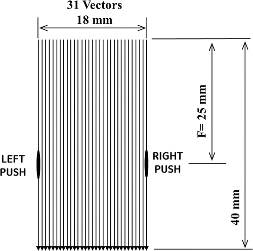
The Acoustic Radiation force Crawling wave (ARC) experimental investigation was conducted at the University of Rochester. A GE Logiq 9 ultrasound system was modified to collect the data required to generate the synthetic ARC wave displacement time histories. A special research scan sequence format was developed to allow a sequence of pushing and tracking vectors to be fired with the desired timing. The duty cycle of the overall scan sequence was $0.35\%$ to avoid thermal limits of the components. The sequence is designed to provide displacement data for a region of interest (ROI) that is typically about 18 mm, though this can be adjusted. The ROI is made up of 31 vectors or locations for which the data was collected. Figure 6 shows the layout of the ROI. The 31 vectors are spaced equally across the ROI, with a spacing of roughly 0.6 mm. For each vector location there is a series of push and track firings. Figure 7 shows the scan sequence that occurs for each location. These sequences consist of a set of reference firings, a push vector on the left side of the ROI, followed by a series of tracking vectors. This is followed by a pause to maintain the duty cycle below thermal limits. Then a push pulse is fired on the right side of the ROI, and this push is also followed by a series of tracking vectors. These tracking vectors are followed by another pause to maintain the duty cycle. This sequence is repeated for each location in the ROI. The left and right push locations are the same for all the vectors in the ROI, but the tracking locations are moved across the ROI. The tracking vectors are fired at a pulse repetition rate of 2.5 kHz. The entire sequence for all 31 locations takes about 4.5 s to collect. Complex baseband demodulated data (IQ) for each of the reference and tracking vectors was stored for offline processing. The sampling rate of the IQ data is 10 MHz. The IQ data was processed to calculate the axial (toward or away from the transducer) component of the displacement for each location as a function of time.

Figure 6. Region of Interest (ROI) in the experimental set-up. The depth is 40 mm and width is 18 mm. The focal depth is 25 mm. The ROI is made up of 31 vectors or locations where data are collected.

Figure 7. Graphic display of scan sequence at each location. Horizontal axis is time.

A gelatin phantom with homogeneous background (approximately 5% gelatin) and a circular finger inclusion of higher stiffness (approximately 10% gelatin) was constructed. The gelatin phantom with the finger inclusion was scanned using the specially designed scan sequences on the modified GE Logiq 9 using a specially built transrectal probe. Two sets of displacement data were collected in rapid succession using the sequence described above. One generated a pushing force which was peaked on the left side of the region of interest (ROI) and the other generated a pushing force which peaked on the right side of the region of interest. The entire sequence was repeated multiple times and averaged to improve the signal to noise ratio. The end result is two axial displacement vs. time profiles for the 2D ROI, u(x, y, t) and v(x, y, t).

6. Performance test on phantom data

The time trace from each displacement data-set contains 48 time steps with 0.3 ms spacing between samples. We synthetically extend the time trace to 400 time steps setting the displacement equal to zero where we have no data measurements. Then we Fourier Transform the data in time. We use the extended and transformed data from both displacements at 9 frequencies ranging from 175 to 275 Hz with 12.5 Hz spacing to reconstruct the complex modulus with our complex marching p.d.e. solver for Equation (8(8) $$\begin{array}{c}\hfill {\tilde{\mathit{\mu }}}_x{\widehat{u}}_x+{\tilde{\mathit{\mu }}}_y{\widehat{u}}_y+\tilde{\mathit{\mu }}▵\widehat{u}=-{\mathit{\omega }}^2\widehat{u}⟹{\tilde{\mathit{\mu }}}_x+a{\tilde{\mathit{\mu }}}_y+b\tilde{\mathit{\mu }}=c,\end{array}$$(8) ). Unlike the case of synthetic data, we applied scheme (12(12) $$\begin{array}{c}\hfill ({\overline{A}}_i^T{A}_i){\overrightarrow{\widetilde{\stackrel{~}{\mathit{\mu }}}}}_{i+1}={\overline{A}}_i^T{\overrightarrow{g}}_i.\end{array}$$(12) ) instead of (13(13) $$\begin{array}{c}\hfill (D+{\overline{A}}_i^T{A}_i){\overrightarrow{\widetilde{\stackrel{~}{\mathit{\mu }}}}}_{i+1}={\overline{A}}_i^T{\overrightarrow{g}}_i,\end{array}$$(13) ). We removed the regularization here since the additional regularization on the numerical solution often gives unacceptably over-regularized results from the exceptionally noisy measured phantom data. The acceptance criteria of numerical results comes from the comparison between our numerical recoveries and the targeted viscoelastic parameters used in [50]. After we obtained the real and the imaginary parts of the complex modulus, we use a total variation minimization procedure (see [51]) to improve the contrast between the high speed and background regions.

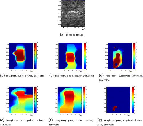
In Figure 8, we present the recovery of the real and imaginary parts of complex shear modulus for this finger inclusion phantom from the complex marching p.d.e. solver and the Algebraic Inversion method together with the B-mode image. For each image, the vertical axis extends from 0.0192 to 0.0338 m with a discretization of 0.000077m while the horizontal axis extends from 0.003 to 0.015 m with a discretization of 0.0006 m. The lower bound of the colourbar is 15 m/s and the upper bound of the colourbar is 40 m/s. The frequency content utilized in this recovery is obtained at 243.75 and 268.75 Hz. Compared with the Algebraic Inversion result, the linear hyperbolic solver with two data-sets has a recovery that is more consistent with the size and location of the inclusion. The location of the recovery is however somewhat shifted. Notice that the real part of reconstruction results obtained with the complex marching p.d.e. solver and two data-sets in these two different frequencies exhibit a better correlation with the B-mode image than the imaginary part of the recoveries. This is consistent with the results from synthetic data as the imaginary part of the complex modulus is generally more difficult to reproduce than the real part.

Figure 8. Recovery from phantom data: (a) B-mode image; (b) real part, p.d.e. solver at 243.75 Hz; (c) real part, p.d.e. solver at 268.75 Hz; (d) real part, Algebraic Inversion at 268.75 Hz; (e) imaginary part, p.d.e. solver at 243.75 Hz; (f) imaginary part, p.d.e. solver at 268.75 Hz; (g) imaginary part, Algebraic Inversion at 268.75 Hz. The units for the shear modulus images are KPa.

With the recovery of complex shear modulus $\tilde{\mathit{\mu }}$ at nine different frequencies, we calculate the average value of the real and imaginary parts of the shear modulus inside the inclusion where the location of the inclusion is determined by edge detection in the B-mode image. Then we determine the viscoelastic parameters in all three viscoelastic models by minimizing the error with a least-square fit:$$\mathit{\chi }=\frac{1}{N}\sum _{i=1}^N\sqrt{{[Re(\tilde{\mathit{\mu }}({\mathit{\omega }}_i)-{\tilde{\mathit{\mu }}}_M({\mathit{\omega }}_i))]}^2+{[Im(\tilde{\mathit{\mu }}({\mathit{\omega }}_i)-{\tilde{\mathit{\mu }}}_M({\mathit{\omega }}_i))]}^2},$$

where ${\tilde{\mathit{\mu }}}_M({\mathit{\omega }}_i)$ is the exact model-based complex shear modulus that is determined by:$$\begin{array}{cc}\text{KVFD}:\hfill & {\displaystyle {\tilde{\mathit{\mu }}}_M({\mathit{\omega }}_i)={\mathit{\mu }}_f+{\mathit{\eta }}_f{(i{\mathit{\omega }}_i)}^{{\mathit{\alpha }}_f}}\hfill \\ \hfill & \\ \text{Spring-pot}:\hfill & {\displaystyle {\tilde{\mathit{\mu }}}_M({\mathit{\omega }}_i)={\mathit{\mu }}_s{(i{\mathit{\omega }}_i{\mathit{\tau }}_s)}^{{\mathit{\alpha }}_s}}\hfill \\ \hfill & \\ \text{Zener}:\hfill & {\displaystyle {\tilde{\mathit{\mu }}}_M({\mathit{\omega }}_i)={\mathit{\mu }}_1+\frac{{\mathit{\mu }}_{2}i{\mathit{\omega }}_i\mathit{\tau }}{i\mathit{\omega }\mathit{\tau }+1}}\hfill \end{array}$$

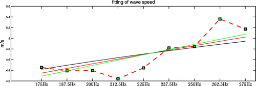
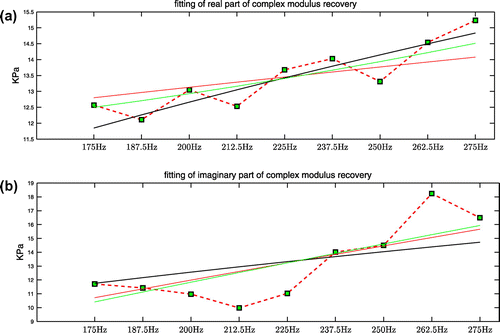
with ${\mathit{\mu }}_f$, ${\mathit{\eta }}_f$, ${\mathit{\alpha }}_f$, ${\mathit{\mu }}_s$, ${\mathit{\tau }}_s$, ${\mathit{\alpha }}_s$, ${\mathit{\mu }}_1$, ${\mathit{\mu }}_2$ and $\mathit{\tau }$ being the undetermined parameters. In Figure 9, the average value of the real and imaginary parts of the complex shear modulus recovery inside the inclusion is plotted against frequency together with the fitted curves for all three viscoelastic models. The plots of the averaged values exhibit an increasing trend with the increase of frequency. We give our fitting results of the viscoelastic parameters in Table 1. We note that the best-fit curves capture the increasing trend of the shear modulus values. In Figure 10, for completeness, we show the wave speed plot calculated from the average complex modulus values using a local plane wave assumption [35], along with the wave speed plots calculated from the best-fit complex modulus curves using a local plane wave assumption:$$c(\mathit{\omega })=\frac{1}{Re\sqrt{\frac{1}{\tilde{\mathit{\mu }}(\mathit{\omega })}}}.$$

In Figure 9, the average value of the real and imaginary parts of the complex shear modulus recovery inside the inclusion is plotted against frequency together with the fitted curves for all three viscoelastic models. The plots of the averaged values exhibit an increasing trend with the increase of frequency. We give our fitting results of the viscoelastic parameters in Table 1. We note that the best-fit curves capture the increasing trend of the shear modulus values.

Table 1. Fitted viscoleastic parameters.

KVFD model	${\mathit{\mu }}_f$	${\mathit{\eta }}_f$	${\mathit{\alpha }}_f$
Value	10.03 KPa	0.0.03 KPa s	0.84
FD model	${\mathit{\mu }}_s$	${\mathit{\tau }}_s$	${\mathit{\alpha }}_s$
Value	5.18 KPa	0.01s	0.50
SLS model	${\mathit{\mu }}_1$	${\mathit{\mu }}_2$	$\mathit{\tau }$
Value	11.07 KPa	77.13 KPa	0.0001 s

Figure 9. Average value inside the inclusion and corresponding fitted curves from all three viscoelastic models: (a) real part; (b) imaginary part; red curve is KVFD model, black curve is SP Model, green curve is Zener Model, dotted red line with green blocks is the averaged value inside the inclusion.

Figure 10. Wave speed calculated from average complex modulus values in the inclusion, along with wave speed calculated from best-fit complex modulus curves.

7. Comparison with phase wave speed

In the previous sections, we used the two data-sets to recover the complex shear modulus. In this section, we compare those results to the results obtained when we combine the two data-sets in a different way and recover the phase wave speed.

The two data-sets can be combined to create a synthetic interference pattern. The idea here is to obtain something similar to a crawling wave using two independently collected data-sets. We apply the delay/add procedure described above to synthetically extend each data-set in time, using a time shift of $N\mathrm{\Delta }t$, obtaining$$u_N(x,y,t)=\sum _{n}u(x,y,t-nN\mathrm{\Delta }t),v_N(x,y,t)=\sum _{n}v(x,y,t-nN\mathrm{\Delta }t).$$

After filtering around the repetition frequency ${\mathit{\omega }}_N=2\mathit{\pi }/(N\mathrm{\Delta }t)$, we have$$\begin{array}{cc}\hfill {\tilde{u}}_N(x,y,t)& \approx a_N(x,y)cos[{\mathit{\omega }}_N(t+{\mathit{\varphi }}_N(x,y))],\hfill \\ \hfill {\tilde{v}}_N(x,y,t)& \approx b_N(x,y)cos[{\mathit{\omega }}_N(t-{\mathit{\phi }}_N(x,y))].\hfill \end{array}$$

The synthetic interference pattern is computed as the variance over one period of the sum of the left time trace and a time-delayed version of the right time trace:$$w_N(x,y,t)=\frac{1}{N\mathrm{\Delta }t}{\int }_{t_0}^{t_0+N\mathrm{\Delta }t}{[{\tilde{u}}_N(x,y,s)+{\tilde{v}}_N(x,y,t+s)]}^2\mathrm{d}s.$$

After filtering to remove the zero-frequency terms, we have$${\tilde{w}}_N(x,y,t)\approx a_N(x,y)b_N(x,y)cos[{\mathit{\omega }}_N(-t+{\mathit{\varphi }}_N(x,y)+{\mathit{\phi }}_N(x,y))].$$

Thus the phase wave speed of the interference pattern is$$c_N(x,y)=\frac{1}{\left|\mathrm{\nabla }{\mathit{\varphi }}_N(x,y)+\mathrm{\nabla }{\mathit{\phi }}_N(x,y)\right|}=\frac{c_s(x,y;{\mathit{\omega }}_N)}{2\left|cos(\mathit{\theta }(x,y)/2)\right|},$$

where $c_s$ is the shear wave speed and $\mathit{\theta }$ is the angle between $\mathrm{\nabla }{\mathit{\varphi }}_N$ and $\mathrm{\nabla }{\mathit{\phi }}_N$. This relation is similar to the relation between the crawling wave speed and shear wave speed in [49].

We recover the interference pattern phase wave speed using either an $L^1$-minimization phase-unwrapping method or a local cross-correlation method. Both of these methods are described in [49]. We approximate the angle $\mathit{\theta }$ by 0, and then we obtain an approximation of the shear wave speed using$$c_s\approx 2c_N.$$

In this case, $\mathit{\theta }\approx 0$ is a reasonable assumption because the two waves are nearly plane waves propagating in opposite directions in the imaging region. If this were not the case, we would recover the shear wave speed from the interference pattern using the method described in [36].

In Figure 11, we show the phase wave speed images that we obtain from the interference pattern using time shifts $N\mathrm{\Delta }t=12\mathrm{\Delta }t$ and $N\mathrm{\Delta }t=8\mathrm{\Delta }t$. These time shifts correspond to repetition frequencies of ${\mathit{\omega }}_N=2\mathit{\pi }\ast 277.7$ and ${\mathit{\omega }}_N=2\mathit{\pi }\ast 416.6$, respectively. 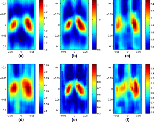Since the images obtained from the $L^1$-minimization phase unwrapping method and the local cross-correlation method are nearly identical, we only show one set of images. These images illustrate that we are able to identify the stiff region using the phase wave speed method, and that we are able to capture the frequency dependence of the phase wave speed. We note that the inclusion can appear elongated in the vertical direction. This happens occasionally for the complex modulus recovery method presented in the previous sections of this paper. However, this elongation happens much more frequently in the phase wave speed recoveries. The source of this elongation is still under investigation.

Figure 11. B-mode image (left) and recovered shear wave speed images using repetition frequencies 277.7 Hz (left) and 416.6 Hz (right), corresponding to time shifts of $N=12$ time steps and $N=8$ time steps, respectively. The units on the horizontal and vertical axes are meters and the units on the colourbar are m/s.

8. Conclusion and future work

We developed a linear explicit-implicit hyperbolic solver for recovering the complex shear modulus from a first-order complex p.d.e. model. We show the numerical scheme is stable with a combination of multiple displacement data-sets and a modified Tikhonov regularization term. Compared with the Algebraic Inversion method previously investigated (see [39]), the linear hyperbolic p.d.e. solver is more stable when the shear modulus is rapidly changing. To preserve the sharp contrast of the shear modulus between the phantom inclusion and the gel background, we applied the complex p.d.e. solver to the phantom data-sets without regularization. The growth of the numerical solution is under control and better reconstructions of the shape and size of the inhomogeneity have been yielded than the Algebraic Inversion method. Compared with the phase wave speed recovered from the synthetic interference pattern, the complex modulus recoveries show less elongation of the inclusion in the vertical direction. The average value of the real and imaginary parts of the complex shear modulus recoveries exhibits frequency dependence consistent with viscoelastic models. We have also provided viscoelastic parameter choices for three specific viscoelastic models by a least-square fitting of the complex shear modulus recovery. For the gel phantom experiments, all three models show a similar qualitative trend for the frequency-dependent complex shear modulus.

Acknowledgements

The authors would like to thank Ning Zhang, Ben Szajewski, and Yixiao Zhang, who are former students at Rensselaer and Dr. Antoinette M. Maniatty and Dr. Assad A. Oberai in MANE of RPI for useful discussions.

Additional information

Funding

The project was partially supported by NIH [grant number R01AG029804]. J. McLaughlin and A. Thomas were partially supported by ONR [grant number N000 14-08-1-0432]. The contents of this paper are solely the responsibility of the authors and do not necessarily represent the official views of ONR and NIA. A. Thomas was also partially supported by a NPSC Fellowship. J. McLaughlin and A. Thomas benefited from their participation during Fall, 2010, semester special program on inverse problems at MSRI.

Notes

No potential conflict of interest was reported by the authors.

Current address: ThingWorx Analytics 550 E. Swedesford Rd. 260, Wayne, PA 19087, USA.

References

- Barbone PE, Bamber JC. Quantitative elasticity imaging: what can and cannot be inferred from strain images. Phys Med Biol. 2002;47:2147–2164.
- Oberai A, Gokhale N, Doyley M, et al. Evaluation of the adjoint equation based algorithm for elasticity imaging. Phys Med Biol. 2004;49:2955–2974.
- Konafagou EE, Harrigan T, Ophir J. Shear strain estimation and lesion mobility assessment in elastography. Ultrasonics. 2000;38:400–404.
- Thitaikumar A, Ophir J. Effect of lesion boundary conditions on axial strain elastograms: a parametric study. Ultrasound Med Biol. 2007;33(9):1463–1467.
- Ophir J, Céspedes EI, Ponnekanti H, et al. Elastography: a quantitative method for imaging the elasticity of biological tissue. Ultrason Imaging. 1991;13:111–134.
- O’Donnell M, Skovoroda AR, Shapo BM, et al. Internal displacement and strain imaging using ultrasonic speckle tracking. IEEE Trans Ultrason Ferroelec Freq Control. 1994;41:314–325.
- Sugimoto T, Ueha S, Itoh K. Tissue hardness measurement using the radiation force of focused ultrasound. Proc IEEE Ultrason Symp. 1990;1:1377–1380.
- Parker KJ, Fu D, Gracewski SM, et al. Vibration sonoelastography and the detectability of lesions. Ultrasound Med Biol. 1998;24:1937–1947.
- Wu Z, Taylor LS, Rubens DJ, et al. Sonoelastographic imaging of interference patterns for estimation of the shear velocity of homogeneous biomaterials. Phys Med Biol. 2004;49:911–922.
- Wu Z, Rubens DJ, Parker KJ. Sonoelastographic imaging of interference patterns for estimation of the shear velocity distribution in biomaterials. J Acoust Soc Am. 2006;120:535–545.
- Maleke C, Luo J, Konofagou EE. 2d simulation of the amplitude-modulated harmonic motion imaging (AM-HMI) with experimental validation. In: IEEE International Ultrasonics Symposium. New York, NY; 2007 Oct 28-31. p. 681–706.
- Curiel L, Souchon R, Rouviere O, et al. Elastography for the follow-up of high-intensity focused ultrasound prostate cancer treatment: initial comparison with MRI. Ultrasound Med Biol. 2005;31:1461–1468.
- Fatemi M, Greenleaf JF. Ultrasound-stimulated vibro-acoustic spectrography. Science. 1998;280:82–85.
- Greenleaf J, Fatemi M, Insana M. Selected methods for imaging elastic properties of biological tissues. Annu Rev Biomed Eng. 2003;5:57–58.
- Manduca A, Lake DS, Ehman RL. Improved inversion of MR elastography images by spatio-temporal directional filtering. Proc SPIE Int Soc Opt Eng. 2003;5032:445–452.
- Ehman RL, Manducca A, McLaughlin JR, et al. Variance controlled shear stiffness images for MRE data. In: IEEE International Symposium on Biomedical Imaging: Macro to Nano. Arlington; 2006. p. 960–963.
- Sinkus R, Siegmann K, Xydeas T, et al. MR elastography of breast lesions: understanding the solid/liquid duality can improve the specificity of contrast-enhanced MR mammography. Magn Reson Med. 2007;58:1135–1144.
- Sarvazyan A, Rudenko OV, Swanson SD, et al. Shear wave elasticity imaging a new ultrasonic technology of medical diagnostics. Ultrasound Med Biol. 1998;24:1419–1435.
- Nightingale KR, McAleavey SA, Trahey GE. Shear wave generation using acoustic radiation force: in vivo and ex vivo results. Ultrasound Med Biol. 2003;29(2):1715–1723.
- Bercoff J, Tanter M, Fink M. Supersonic shear imaging: a new technique for soft tissue elasticity mapping. IEEE Trans Ultrason Ferroelectr Freq Control. 2004;19:396–409.
- Sandrin L, Tanter M, Catheline S, et al. Shear modulus imaging with 2-d transient elastography. IEEE Trans Ultrason Ferroelectr Freq Control. 2002;49:426–435.
- Tanter M, Bercoff J, Athanasiou A, et al. Quantitative assessment of breast lesion viscoelasticity: initial clinical results using supersonic shear imaging. Ultrasound Med Biol. 2008;34(9):1373–1386.
- Palmeri ML, McAleavey SA, Trahey GE, et al. Ultrasonic tracking of acoustic radiation force-induced displacements in homogeneous media. IEEE Trans Ultrason Ferroelectr Freq Control. 2006;53(7):1300–1313.
- Palmeri ML, Wang MH, Dahl JJ, et al. Quantifying hepatic shear modulus in vivo using acoustic radiation force. Ultrasound Med Biol. 2008;34(4):546–558.
- Palmeri ML, Dahl JJ, Macleod DB, et al. On the feasibility of imaging peripheral nerves using acoustic radiation force impulse imaging. Ultrasound Imaging. 2009;31(3):172–182.
- Chen S, Urban MW, Pislaru C, et al. Shearwave dispersion ultrasound vibrometry (SDUV) for measuring tissue elasticity and viscosity. IEEE Trans Ultrason Ferroelectr Freq Control. 2009 Jan;56(1):55–62.
- Parker KJ, Doyley MM, Rubens DJ. Imaging the elastic properties of tissue: the 20 year perspective. Phys Med Biol. 2011;56:R1–R29.
- Zhang M, Nigwekar P, Castaneda B, et al. Quantitative characterization of viscoelastic properties of human prostate correlated with histology. Ultrasound Med Biol. 2008;34(7):1033–1042.
- Sinkus R, Tanter M, Xydeas T, et al. Viscoelastic shear properties of in vivo breast lesions measured by MR elastography. Magn Reson Imaging. 2005;23(2):159–165.
- Chen S, Urban MW, Greenleaf JF, et al. Quantification of liver stiffness and viscosity with SDUV: in vivo animal study. In: IEEE International Ultrasonics Symposium Proceeding. Beijing; 2008. p. 654–657.
- Klatt D, Hamhaber U, Asbach P, et al. Noninvasive assessment of the rheological behavior of human organs using multifrequency MR elastography: a study of brain and liver viscoelasticity. Phys Med Biol. 2007;52:7281–7294.
- Koeller RC. Applications of fractional calculus to theory of viscoelasticity. J Appl Mech Trans ASME. 1984;51:299–307.
- Suki B, Barabasi AL, Lutchen KR. Lung tissue viscoelasticity: a mathematical framework and its molecular basis. J Appl Physiol. 1994;76:2749–2759.
- Taylor LS, Lerner AL, Rubens DJ, et al. A Kelvin-Voigt fractional derivative model for viscoelastic characterization of liver tissue. In: ASME International Mechanical Engineering Congress and Exposition. New Orleans; 2002.
- Fung Y. Biomechanics: mechanical properties of living tissue. New York (NY): Springer-Verlag; 1993.
- Lin K, McLaughlin JR, Renzi D, et al. Shear wave speed recovery in sonoelastography using crawling wave data. J Acoust Soc Am. 2010;128:88–97.
- Jensen JA, Svendsen NB. Calculation of pressure fields from arbitrarily shaped, apodized, and excited ultrasound transducers. IEEE Trans Ultrason Ferroelec Freq Control. 1992;39:262–267.
- Jensen JA. Field: a program for simulating ultrasound systems, paper presented at the 10th nordic-baltic conference on biomedical imaging. Med Biol Eng Comput. 1996;34(1):351–353.
- Lin K, McLaughlin JR. An error estimate on the direct inversion model in shear stiffness imaging. Inverse Prob. 2009;25:075003.
- Lin K, McLaughlin JR, Zhang N. Log-elastographic and non-marching full inversion schemes for shear modulus recovery from single frequency elastographic data. Inverse Prob. 2009;25:075004.
- Hwang YH. Upwind scheme for non-hyperbolic systems. J Comput Phys. 2003;192:643–676.
- McLaughlin JR, Zhang N, Manduca A. Calculating tissue shear modulus and pressure by 2d log-elastographic methods. Inverse Prob. 2010;26:085007.
- Zhang YX, Oberai A, Barbone P, et al. Solution of the time-harmonic viscoelastic inverse problem with interior data in two dimensions. Int J Numer Methods Eng. 2012;92:1100–1116.
- Doyley MM. Model-based elastography: a survey of approaches to the inverse elasticity problem. Phys Med Biol. 2012;57(3):35–73.
- Thomas JW. Numerical partial differential equations: finite difference methods. New York (NY): Springer; 1995.
- Nyborg WLM. Physical acoustics. New York (NY): Academic Press; 1965.
- Collino F, Tsogka C. Application of the perfectly matched absorbing layer model to the linear elastodynamic problem in anisotropic heterogeneous media. Geophysics. 2001;66(1):294–307.
- Anderssen R, Hegland M. For numerical differentiation, dimensionality can be a blessing!. Math Comput. 1999;68(227):1121–1141.
- Lin K, McLaughlin JR, Thomas A, et al. Two-dimensional shear wave speed and crawling wave speed recoveries from in vitro prostate data. J Acoust Soc Am. 2010, submitted for publication.
- Lee RH, Szajewski BA, Hah Z, et al. Modeling shear waves through a viscoelastic medium induced by acoustic radiation force. Int J Numer Methods Biomed Eng. 2012;28:678–696.
- McLaughlin JR, Renzi D. Shear wave speed recovery in transient elastography and supersonic imaging using propagation fronts. Inverse Prob. 2006;22:681–706.