Application of the photoacoustic technique for temperature measurements during hyperthermia

ABSTRACT

Non-invasive monitoring of tissues’ temperatures is necessary for some diagnostic and therapeutic applications. Photoacoustic is a new hybrid biomedical imaging technique, combining the high-contrast of optical properties with the high spatial resolution of ultrasound. The estimation of model parameters that are temperature dependent was used in this work to indirectly measure the temperatures of tissues, as the solution of an inverse problem within the Bayesian framework of statistics. A two-dimensional case was examined, which is related to the hyperthermia treatment of cancer with laser heating in the near infrared range. Simulated measurements were used in the inverse analysis. The Markov Chain Monte Carlo method provided accurate estimation of the spatial distribution of the Gruneisen parameter and the temperature distribution in the region of interest could be recovered with discrepancies smaller than 0.03°C.

KEYWORDS:

• Inverse problems
• nonintrusive temperature measurements
• photo-acoustics
• Markov chain Monte Carlo method
• Bayesian estimator

SUBJECT CLASSIFICATIONS:

• 62F15
• 62H12
• 62M05
• 62P10
• 62P30

Nomenclature
cp	=	specific heat
DT	=	thermal diffusivity
Hh	=	volumetric heat source resulting from the absorbed optical energy
k	=	thermal conductivity
$p$	=	photoacoustic pressure
$Q_{\mathrm{met}}$	=	metabolic heat generation per unit volume
T	=	temperature
$T^{\ast }$	=	temperature variation
t	=	time
tpulse	=	laser pulse duration
u	=	acoustic particle velocity
WL	=	tumour width
${\omega }_b$	=	blood perfusion coefficient
x,y	=	spatial variables
Y	=	vector of measurements

Greek Symbols
$\alpha$	=	Metropolis-Hastings ratio
$\beta$	=	thermal expansion coefficient
$\delta$	=	Dirac delta function
γ	=	hyperparameter
Γ	=	Gruneisen's parameter
$\mathrm{\Phi }$	=	laser fluence rate
${\mu }_a$	=	light absorption coefficient
${\nu }_s$	=	sound speed
π	=	probability distribution function
Π(P)	=	vector with the solution of the direct problem with known P
ρ	=	density
ρ'	=	acoustic density
Σ	=	covariance matrix
$\omega$	=	perfusion coefficient

Superscripts
t	=	state of the Markov chain

Introduction

Noninvasive temperature measurements of the human body are useful in clinical diagnostics and therapy monitoring. Inflammations, infections and cancerous cells locally increase the temperature as a result of larger metabolism. For example, some researchers used temperature measurements for the diagnosis of breast cancer [1,2]. Moreover, during the hyperthermia treatment of cancer, the accurate knowledge of the temperature inside the tumour and in the surrounding tissues is necessary for an effective therapy, with minimal damage to normal cells. Indeed, healthy tissues should not be exposed to temperatures exceeding 41°C in order to avoid thermal damage [3–10].

The detection of electromagnetic radiation (microwave radiometry) emitted from the human body was applied as non-invasive thermometry [11,12]. Despite the temperature sensitivity of 0.1°C, microwave radiometry exhibits relative poor temporal and spatial resolution of the measurements, as well as susceptibility to interference from other electrical signals [10,11]. Another method applied to non-invasive thermometry was magnetic resonance. In this method, the effects of temperature on several physical parameters that influence the measured signals, including the water proton chemical shift [13,14], the spin-lattice relaxation time [15,16] and the water diffusion coefficient [17], were used for the measurement of temperature. An investigation about the temperature-dependence of the spin-lattice relaxation time revealed that such quantity varies with the type of tissue and is approximately linear in the temperature range from 20°C to 50°C [16]. The molecular water diffusion coefficient in tissues is highly sensitive to temperature variations and has been used for non-invasive in-vivo thermometry [18]. Delannoy et al [17] found the agreement between invasive and non-invasive temperature measurements with magnetic resonance to be better than 0.2°C in a gel phantom. Germain et al. [19] used magnetic resonance based on the water proton chemical shift for monitoring the temperature variation of a tumour with high sensitivity during thermal therapy. Despite its current application and feasibility, magnetic resonance thermometry presents some disadvantages, including high cost, unreliable temperature measurements in tissues rich in fat and sensitivity to motion [20]. Methods based on the temperature dependence of ultrasonic properties have also been used for non-invasive thermometry of tissues in-vivo. Seip and Ebbini [21] showed a relation between temperature changes and frequency changes in the spectrum of reflected ultrasound pulses. In another investigation, echo shifts were applied to measure the temperature in High Intensity Focused Ultrasound (HIFU) therapy, in a turkey breast muscle [22]. Although such results were consistent with theoretical predictions, ultrasound methods suffer from low sensitivity of physical properties with respect to temperature variations [22].

Photoacoustic (PA) techniques have recently been applied for non-invasive medical diagnosis and imaging, based on the generation of acoustic pressure waves from the absorption of light energy in the tissues. The sound speed, the thermal expansion coefficient and the specific heat are three parameters that exhibit temperature dependence in the photoacoustic model. These parameters compose the so-called Gruneisen parameter [23–30]. Therefore, the pressure amplitudes of the generated acoustic waves in photoacoustics are related to the temperature through the Gruneisen parameter. An advantage of the photoacoustic technique is that the optical properties practically do not depend on temperature, particularly in the range related to the hyperthermia treatment of cancer [31]. By using the photoacoustic technique, Haixin et al. [32] could measure the spatial distribution of temperature in deep tissues, by using as reference the temperature of a thermocouple. Also, Sergey [33] performed experiments to correlate the photoacoustic signal amplitude to temperature in different tissues, such as chicken breast (skeletal muscle), porcine lard (fatty tissue) and porcine liver (richly perfused tissue), in the temperature range from 25°C to 80°C, during heating and cooling. Wu et al. [34] used photoacoustic imaging for temperature measurements during High Intensity Focused Ultrasound (HIFU) therapy. They conducted experiments in ex-vivo bovine tissues, in order to characterize the linear dependence of the photoacoustic image with the local temperature and, consequently, obtain a high-precision, high-resolution, real-time temperature map [34]. In another study, photoacoustic thermometry was utilized during prostate cryoablation in a live canine model; an accuracy of ± 2°C was achieved for the range of temperatures from −5°C to 35°C [35]. Yu Liaoa et al. [36] proposed a new method to improve the accuracy of photoacoustic thermometry by using measurements at two wavelengths. A resolution of about 1°C in the range from 23°C to 48°C in ex-vivo pig blood was obtained with their method [36].

In the above referenced studies on photoacoustic thermometry, the correlation of the acoustic signal and the Gruneisen parameter relied on invasive temperature measurements. Also, these studies directly associated changes in the photoacoustic signals to temperature, due to the variation of the sound speed and thermal expansion coefficient, but did not consider the estimation of these parameters. As a non-invasive thermometry method, the use of inverse analysis to indirectly estimate temperature through the estimation of the sound speed and thermal expansion coefficient was developed by the authors in reference [37]. Our previous work is extended here for a two-dimensional case related to the hyperthermia treatment of cancer, with laser heating in the near infrared range, where the spatial variation of the Gruneisen parameter is estimated in the region. Simulated measurements of the ultrasound pressure waves are used in the photoacoustic inverse analysis within the Bayesian framework of statistics [38]. A Markov chain Monte Carlo (MCMC) method, coded in the form of the Metropolis-Hastings algorithm [38–41], is used for the estimation of the Gruneisen parameter, which thus serves as an indirect measurement of the spatial variation of the temperature in the tissue.

Physical problem and mathematical formulation

The photoacoustic technique relies on pressure acoustic waves generated from the light energy absorbed by the chromophores in a tissue, during a time period smaller than the thermal relaxation time. This so-called thermal confinement condition causes an adiabatic local absorption of the light energy. The localized heating results in temperature increases of the order of 10⁻³ Kelvin, which generates pressure waves with magnitudes of 10³ Pascal [42]. The thermal confinement condition is valid for [43]: (1) $t_{\mathrm{pulse}}<\frac{d_c^2}{4D_T}$(1) where t_pulse is the laser pulse duration, d_c is the desired spatial resolution and D_T is the thermal diffusivity.

The physical problem examined in this paper is related to the hyperthermia treatment of cancer, with heating imposed by a laser in the near infrared range. A two-dimensional region is considered here (see Figure 1). During the hyperthermia treatment, the laser energy is absorbed by the tissues in order to raise their temperatures to levels that make the cells more vulnerable to other kinds of treatment, like chemotherapy or radiotherapy. At a specific time, another laser pulse is applied to generate the photoacoustic waves that are used to measure the temperature in the region, through the measurements of ultrasound transducers, as illustrated by Figure 1. These transducers are nonintrusive and located over the same surface where the heating is imposed. While the bioheat transfer phenomena related to the hyperthermia treatment are of the order of minutes, the photoacoustic phenomena are of the order of 10⁻⁶ s. Hence, the temperatures measured through the photoacoustic technique can be assumed as instantaneous.

Figure 1. Sketch of the physical problem.

The two-dimensional linear mathematical formulation of the photoacoustic problem in soft biological tissues is given by: $\left({\mathrm{\nabla }}^2-\frac{1}{{v_s}^2}\frac{{\mathrm{\partial }}^2}{\mathrm{\partial }{t}^2}\right)p(x,y,t)=-\frac{\beta }{c_p}\frac{\mathrm{\partial }{H}_h(x,y,t)}{\mathrm{\partial }t}$ (2) $\text{in}-\frac{W}{2}<x<\frac{W}{2};-\frac{H}{2}<y<\frac{H}{2};t>0$(2)

The source term of equation (2) is the time derivative of (3) $H_h(x,y,t)=H(x,y)\delta \left(t\right)$(3) where H(x,y) is the local energy deposited per unit volume by the photoacoustic laser pulse and δ(t) is the Dirac delta function. Hence, we assume that the laser pulse used for the photoacoustic measurements is instantaneously absorbed by the tissues, which is consistent with the thermal confinement condition [43]. Therefore, the effects of the laser pulse are taken into account through the initial pressure distribution, $p_0(x,y,T)$, at t = 0. By assuming that the volume expansion is negligible, the initial photoacoustic pressure can be written as [37]: (4) $p_0(x,y,T)=\beta (x,y,T)\rho (x,y,T)v_s^2(x,y,T)T^{\ast }(x,y,0)$(4) where $T\equiv T(x,y,t)$ is the local temperature. The initial temperature rise, $T^{\ast }(x,y,0)$, can be expressed as a function of the absorbed laser flux [44], that is, (5) $T^{\ast }(x,y,0)=\frac{{\mu }_a(x,y)}{\rho (x,y,T)c_p(x,y,T)}\mathrm{\Phi }(x,y)$(5) By combining equations (4) and (5), the initial photoacoustic pressure can be written as a function of the laser fluence rate, $\mathrm{\Phi }(x,y)$ as: (6) $p_0(x,y,T)={\mu }_a(x,y)\mathrm{\Gamma }(x,y,T)\mathrm{\Phi }(x,y)$(6) where (7) $\mathrm{\Gamma }(x,y,T)=\frac{v_s^2(x,y,T)\beta (x,y,T)}{c_p(x,y,T)}$(7) is the Gruneisen parameter [44]. Therefore, the Gruneisen parameter, and thus the photoacoustic signal, is directly related to the local temperature, since the speed of sound, $v_s^2(x,y,T)$, the thermal expansion coefficient, $\beta (x,y,T)$, and the specific heat, $c_p(x,y,T)$, are functions of the local temperature T(x,y,t).

Under the hypotheses that the medium is isotropic, that there is no net flow and that shear waves can be neglected [45], equation (2) can be re-written as three equations, corresponding to momentum conservation, mass conservation and an equation of state, which involve acoustic pressure, p, acoustic particle velocity, u, and acoustic density, ρ’, respectively as [46]: (8.a) $\frac{\mathrm{\partial }\mathbf{\text{u}}(x,y,T)}{\mathrm{\partial }t}=-\frac{1}{\rho (x,y,T)}\mathrm{\nabla }p(x,y,T)\text{in}-\frac{W}{2}<x<\frac{W}{2};-\frac{H}{2}<y<\frac{H}{2};t>0$(8.a) (8.b) $\frac{\mathrm{\partial }{\rho }^{\mathrm{\prime }}(x,y,T)}{\mathrm{\partial }t}=-\rho (x,y,T)\mathrm{\nabla }\cdot \mathbf{\text{u}}(x,y,T)\text{in}-\frac{W}{2}<x<\frac{W}{2};-\frac{H}{2}<y<\frac{H}{2};t>0$(8.b) (8.c) $p(x,y,T)={\rho }^{\mathrm{\prime }}(x,y,T){\nu }_s^2(x,y,T)\text{in}-\frac{W}{2}<x<\frac{W}{2};-\frac{H}{2}<y<\frac{H}{2};t>0$(8.c) with the initial conditions given by equation (6) for pressure and u = ρ’ = 0, in the region at t = 0. In order to generate an infinite domain propagation, artificial absorbing layers, called perfect match layers, were added to the computational domain at the lateral boundaries at $x=\pm W/2$ [47]. Other artificial water layers were added to the computational domain at the bottom and top boundaries, for the perfect ultrasound coupling between the medium and the surroundings [37].

For the bioheat transfer model related to the hyperthermia treatment under analysis, with heating imposed by a laser in the near infrared range, we followed the same mathematical formulation used in references [6,48,49]. The hyperthermia laser fluence rate was computed with a δ-P1 approximation method [50,51], where a flat laser flux was imposed within $-\frac{W_L}{2}<x<\frac{W_L}{2}$ at y = 0. The temperature distribution in the medium was modelled with Pennes' equation [52]. The bottom and top surfaces were assumed to exchange heat with the surrounding media by convection, while the lateral surfaces were assumed insulated. Details of the bioheat transfer model are avoided for the sake of brevity, but they can be readily found in [48–50].

Inverse problem

The inverse problem examined in this work deals with the estimation of the physical parameters, P, that appear in the mathematical formulation of the photoacoustic problem given by equations (8), by using measurements of the acoustic pressure waves, Y, obtained with transducers located at the bottom surface of the region, as illustrated by Figure 1. Our focus is on the estimation of the spatial distribution of the Gruneisen parameter, given by equation (7), since it can be directly related to the local temperature in the region at a specific time.

The present inverse problem is solved within the Bayesian framework, where all quantities appearing in the mathematical formulation of the physical problem are modelled as random variables, by exploring the posterior density function, which is the conditional probability distribution of the unknown parameters given the measurements [39,40]. The posterior density function is obtained from the information provided by the likelihood function, which is the model for the measurement errors, and from the prior probability distribution, which represents the information about the parameters before the measurements are available.

By assuming that the measurement errors are additive, Gaussian, with zero mean, known covariance matrix (Σ) and independent of the parameters, their probability density function is given by [44–47]: (9) $\pi \left(\mathbf{\text{Y}}|\mathbf{\text{P}}\right)=(2\text{π}{)}^{-D/2}|\mathrm{\Sigma }{|}^{-1/2}\exp \left\{-\frac{1}{2}{\left[\mathbf{\text{Y}}-\mathrm{\Pi }\right(\mathbf{\text{P}}\left)\right]}^T{\mathrm{\Sigma }}^{-1}\left[\mathbf{\text{Y}}-\mathrm{\Pi }\right(\mathbf{\text{P}}\left)\right]\right\}$(9) which is the likelihood function for the present case, where $\mathbf{\Pi }\left(\mathbf{\text{P}}\right)$ is the solution of the forward problem given by equations (8) with known P, π(Y|P) is the conditional probability of Y given P and $\text{π}=4{\tan }^{-1}\left(1\right)$.

The formal mechanism to combine the new information (measurements) with the previously available information (prior) is Bayes’ theorem [38–41] given by: (10) ${\pi }_{\mathrm{posterior}}\left(\mathbf{\text{P}}\right)=\pi \left(\mathbf{\text{P}}|\mathbf{\text{Y}}\right)=\frac{\pi \left(\mathbf{\text{Y}}|\mathbf{\text{P}}\right)\pi \left(\mathbf{\text{P}}\right)}{\pi \left(\mathbf{\text{Y}}\right)}$(10) where π_posterior(P) is the posterior probability density, π(P) is the prior density, π(Y|P) is the likelihood function and π(Y) is the marginal probability density of the measurements, which plays the role of a normalizing constant.

In this work the posterior distribution is explored by using the Metropolis-Hastings algorithm of the Markov chain Monte Carlo (MCMC) method [38–41]. The implementation of the Metropolis-Hastings algorithm starts with the selection of a proposal distribution $q\left({\mathbf{\text{P}}}^{\ast }|{\mathbf{\text{P}}}^{\left(t\right)}\right)$, which is used to draw a new candidate state ${\mathbf{\text{P}}}^{\ast }$, given the current state ${\mathbf{\text{P}}}^{\left(t\right)}$of the Markov chain. In order to avoid eventual cases that ${\pi }_{\mathrm{posterior}}\left({\mathbf{\text{P}}}^{\left(t\right)}\right)q\left({\mathbf{\text{P}}}^{\ast }|{\mathbf{\text{P}}}^{\left(t\right)}\right)>{\pi }_{\mathrm{posterior}}\left({\mathbf{\text{P}}}^{\ast }\right)q\left({\mathbf{\text{P}}}^{\left(t\right)}|{\mathbf{\text{P}}}^{\ast }\right)$, that is, the process moves from ${\mathbf{\text{P}}}^{\left(t\right)}$ to ${\mathbf{\text{P}}}^{\ast }$more often than the reverse, a probability $\alpha \left({\mathbf{\text{P}}}^{\ast }|{\mathbf{\text{P}}}^{\left(t\right)}\right)$ is introduced so that the reversibility condition is satisfied, that is, (11) ${\pi }_{\mathrm{posterior}}\left({\mathbf{\text{P}}}^{\left(t\right)}\right)q\left({\mathbf{\text{P}}}^{\ast }|{\mathbf{\text{P}}}^{\left(t\right)}\right)\alpha \left({\mathbf{\text{P}}}^{\ast }|{\mathbf{\text{P}}}^{\left(t\right)}\right)={\pi }_{\mathrm{posterior}}\left({\mathbf{\text{P}}}^{\ast }\right)q\left({\mathbf{\text{P}}}^{\left(t\right)}|{\mathbf{\text{P}}}^{\ast }\right)$(11)

Therefore, (12) $\alpha \left({\mathbf{\text{P}}}^{\ast }|{\mathbf{\text{P}}}^{\left(t\right)}\right)=min\left[1,\frac{{\pi }_{\mathrm{posterior}}\left({\mathbf{\text{P}}}^{\ast }\right)q\left({\mathbf{\text{P}}}^{\left(t\right)}|{\mathbf{\text{P}}}^{\ast }\right)}{{\pi }_{\mathrm{posterior}}\left({\mathbf{\text{P}}}^{\left(t\right)}\right)q\left({\mathbf{\text{P}}}^{\ast }|{\mathbf{\text{P}}}^{\left(t\right)}\right)}\right]$(12) where $\alpha \left({\mathbf{\text{P}}}^{\ast }|{\mathbf{\text{P}}}^{\left(t\right)}\right)=1$ when ${\pi }_{\mathrm{posterior}}\left({\mathbf{\text{P}}}^{\left(t\right)}\right)q\left({\mathbf{\text{P}}}^{\ast }|{\mathbf{\text{P}}}^{\left(t\right)}\right)={\pi }_{\mathrm{posterior}}\left({\mathbf{\text{P}}}^{\ast }\right)q\left({\mathbf{\text{P}}}^{\left(t\right)}|{\mathbf{\text{P}}}^{\ast }\right)$. Equation (12) is also called the Metropolis-Hastings ratio. Notice that, for the computation of equation (12), there is no need to know the normalizing constant that appears in the definition of the posterior distribution (see equation 10).

The Metropolis-Hastings algorithm can then be summarized by the following steps [44–48]:

1. Let $t=1$ and start the Markov chain with the initial state ${\mathbf{\text{P}}}^{\left(1\right)}$.

2. Sample a candidate point ${\mathbf{\text{P}}}^{\ast }$from a proposal distribution $q\left({\mathbf{\text{P}}}^{\ast }|{\mathbf{\text{P}}}^{\left(t\right)}\right)$.

3. Calculate the probability $\alpha \left({\mathbf{\text{P}}}^{\ast }|{\mathbf{\text{P}}}^{\left(t\right)}\right)$ with equation (12).

4. Generate a random value $U\sim \text{U}(0,1)$, which is uniformly distributed in (0,1).

5. If $U\le \alpha \left({\mathbf{\text{P}}}^{\ast }|{\mathbf{\text{P}}}^{\left(t\right)}\right)$, set ${\mathbf{\text{P}}}^{(t+1)}$= ${\mathbf{\text{P}}}^{\ast }$. Otherwise, set ${\mathbf{\text{P}}}^{(t+1)}$= ${\mathbf{\text{P}}}^{\left(t\right)}$.

6. Make $t=t+1$ and return to step 2 in order to generate the sequence $\{{\mathbf{\text{P}}}^{\left(1\right)},{\mathbf{\text{P}}}^{\left(2\right)},\dots ,{\mathbf{\text{P}}}^{\left(n\right)}\}$.

In this way, a sequence is generated to represent the posterior distribution and inference on this distribution is obtained from inference on the samples $\{{\mathbf{\text{P}}}^{\left(1\right)},{\mathbf{\text{P}}}^{\left(2\right)},\dots ,{\mathbf{\text{P}}}^{\left(n\right)}\}$. We note that values of ${\mathbf{\text{P}}}^{\left(t\right)}$must be ignored until the chain has not converged to equilibrium (the burn-in period).

For the implementation of the Markov Chain Monte Carlo method, two different non-informative priors were considered for the spatial distribution of the Gruneisen parameter, namely: (i) Total Variation (TV); and (ii) Gaussian Markov Random Field (GMRF) [38,53]. The Total Variation prior is given in the following form: (13) $\pi \left(\mathbf{\text{P}}\right)\propto \exp \left[-\gamma \text{TV}\left(\mathbf{\text{P}}\right)\right]$(13) where, for the Gruneisen parameter Γ, (14) $\begin{array}{rl}\text{TV}\left(\mathbf{\text{P}}\right)& =\sum _{i=2}^{I-1}\sum _{j=2}^{J-1}\mathrm{\Delta }y\left[|\mathrm{\Gamma }(x_i,y_j)-\mathrm{\Gamma }(x_{i+1},y_j)|+|\mathrm{\Gamma }(x_i,y_j)-\mathrm{\Gamma }(x_{i-1},y_j)|\right]\\ & +\mathrm{\Delta }x\left[|\mathrm{\Gamma }(x_i,y_j)-\mathrm{\Gamma }(x_i,y_{j+1})|+|\mathrm{\Gamma }(x_i,y_j)-\mathrm{\Gamma }(x_i,y_{j-1})|\right]\end{array}$(14)

In equation (14), Δx and Δy are the sizes of the finite volumes used in the discretization of the photoacoustic and bioheat transfer problems, that is, W = IΔx and H = JΔy.

The parameter γ in equation (13) represents the uncertainties related to the TV prior and was selected based on numerical experiments, since it cannot be considered as a hyperparameter due to the unknown normalizing constant for this probability distribution [39].

The Gaussian Markov Random Field prior is given by [54]: (15) $\pi \left(\mathbf{P}\right)\propto {\gamma }^{N/2}\exp \left[-\frac{1}{2}\gamma {\mathbf{P}}^T\mathbf{Z}\mathbf{P}\right]$(15) where $\mathbf{Z}={\mathbf{D}}^T\mathbf{D}$. The singular covariance matrix of this prior is given by ${\gamma }^{-1}{\mathbf{Z}}^{-1}$. The matrix D relates the values of the local parameter to those in its neighbourhood, in order to characterize the prior as a Markov random field. In this work, the following difference matrix was selected for D: (16) $\mathbf{D}=\left[\begin{array}{ccccc}-1& 1& & & \\ & -1& 1& & \\ & & \ddots & \ddots & \\ & & & -1& 1\end{array}\right]$(16) which was applied separately in the x and y directions.

For the Gaussian Markov Random field, a hyperprior was assumed for the hyperparameter γ in the form of a Rayleigh distribution, that is, (17) $\pi \left(\gamma \right)=\frac{\gamma }{{\gamma }_0^2}\exp \left[-\frac{1}{2}{\left(\frac{\gamma }{{\gamma }_0^{}}\right)}^2\right]$(17)

Results and discussions

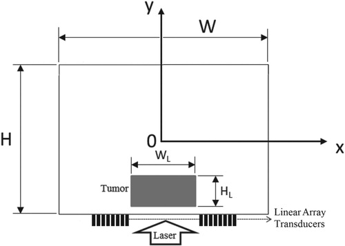
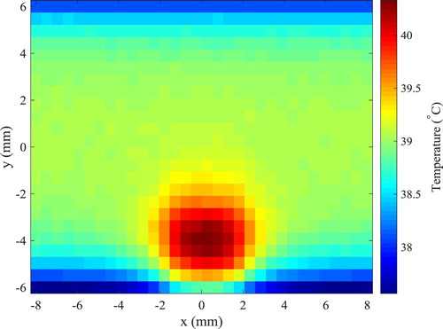
The finite volume method was used to solve the direct problem of hyperthermia, involving light propagation in the tissues and bioheat transfer, with the Alternating Direction-Implicit (ADI) scheme [55], such as in references [6,48,49]. The tissue in the two-dimensional region was supposed as muscle, where the size of the domain was taken as W = 16 mm and H = 12 mm. A rectangular region contained a tumour with W_L = 4 mm of width and H_L = 2.5 mm of height, centred in the x direction and located 0.5 mm underneath the heated surface (y = − 6 mm). This bottom surface was irradiated by a continuous flat laser beam (parallel to the y direction) of 1.9 mJ, at the wavelength of 800 nm and with width W_L = 4 mm (same as the tumour width), in order to increase the temperature in the region during the hyperthermia treatment. The tumour was supposed loaded with gold nanorods (concentration of 3 × 10¹⁵ nanoparticles/m³) of effective radius 11.43 nm and aspect ratio 3.9, with maximum absorption at the wavelength of 800 nm [50,51,58]. With the nanorods, the laser energy used for the hyperthermia treatment was mostly absorbed in the tumour region, thus avoiding that the surrounding healthy tissues be exposed to high temperatures. The absorption coefficients of muscle and tumour at the wavelength of 800 nm were 54 m⁻¹ and 120 m⁻¹, respectively, while the scattering coefficients of these tissues were 6670 m⁻¹ and 6675 m⁻¹, respectively [50,51,56–58]. The thermophysical properties for the muscle and for the tumour are summarized in Table 1. The heat transfer coefficients of the muscle to the surroundings were 6 W/m²K and 10 W/m²K, at the bottom and top boundaries, respectively. The bottom boundary was supposed to exchange heat with air at temperature of 25°C, while the top boundary was supposed to exchange heat with deeper tissues at 37°C. The computer code developed in this work, for the coupled radiation and bioheat transfer forward problem related to the hyperthermia treatment, was verified against the solution obtained with COMSOL®. Based on the solution verification procedure, J = 96 and I = 128 finite volumes were used for the discretization in the y and x directions, respectively. The initial condition for the transient hyperthermia problem was taken as the solution of the steady-state bioheat transfer problem without the laser heating. The temperature distribution in the region after 20 s of continuous heating, during the hyperthermia treatment, is presented by Figure 2. Notice in Figure 2 the larger temperatures in the tumour due to the nanoparticles loaded in this region, which increase the absorption of the laser used for the hyperthermia treatment. Notice also that only a mild hyperthermia treatment is considered in this work, which is in general adjuvant to other treatments, such as chemotherapy and radiotherapy. Hence, the temperatures in the tumour are not so high, so that optical and thermophysical properties can be assumed as constant during treatment. The solution of the present photoacoustic inverse problem is focused on the estimation of the temperature distribution shown by Figure 2, through the estimation of the spatial variation of the Gruneisen parameter.

Figure 2. Temperature distribution after 20 s of the hyperthermia treatment.

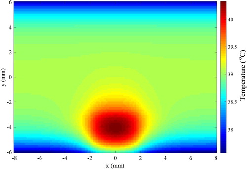
Table 1. Thermophysical properties for muscle and tumour [56].

	$\rho$(kg m^−3)	$c_{\mathrm{p}}$(J kg^−1 K^−1)	$k$(W m^−1K^−1)	$Q_{\mathrm{met}}$(W m^−3)	${\omega }_b$(s^−1)
Muscle	1073.4	3631.1	0.51	684.2	27×10^−4
Tumour	1073.4	3631.1	0.51	3680	63×10^−4

The photoacoustic pressure waves for the solution of the inverse problem were generated from a flat laser pulse of 1.9 mJ, with duration of 9 × 10⁻⁹ s, at the wavelength of 550 nm, also with width of 4 mm centred around x = 0 at the bottom boundary. The effect of nanorods on absorption and scattering coefficients of tumour at this wavelength is negligible [58]. The absorption coefficient and scattering coefficient for muscle and tumour were assumed for this wavelength as 166 m⁻¹ and 8820 m⁻¹, respectively. The problem for the light propagation of this flat laser pulse was also solved with the same code applied to the solution of the hyperthermia problem. The fluence rate resulting from the laser pulse for the photoacoustic problem is presented by Figure 3.

Figure 3. Distribution of fluence rate resulting from the laser pulse for the photoacoustic inverse problem.

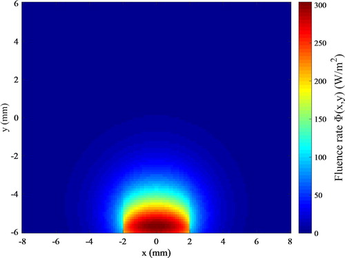
The Matlab toolbox k-Wave [45,59] was then used for the numerical solution of the acoustic problem given by equations (8.a-c). After a grid convergence analysis, the region was discretized with a mesh of 128 grids in the x and y directions and the solution was computed up to 15 µs after the laser pulse. The initial pressure field, generated from the instantaneous absorption of the laser pulse, reaches maximum values of the order of 20 kPa in the tumour region, due to the local larger temperatures resulting from the hyperthermia treatment, as shown by Figure 4.

Figure 4. The initial pressure field $p_0(x,y,T)$ generated by the laser pulse for the photoacoustic inverse problem.

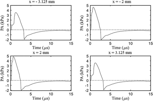
The photoacoustic pressure waves were detected by two linear array transducers, which were located non-intrusively at the bottom boundary (y = − 6 mm) on both sides of the laser irradiation region. Each linear array contained 8 transducers, spaced by 0.375 mm, and started from x = − 2 mm towards the left boundary and from x = 2 mm towards the right boundary (see Figure 1). The transient variation of the photoacoustic pressure at four locations of the transducers, which resulted from the initial pressure field shown by Figure 4 and from the temperature field shown by Figure 2, are presented by Figure 5. This figure shows that peak values at the bottom boundary are of the order of few kPa. The pressures at the transducer positions become negative because of reflections at the bottom boundary, caused by the impedance difference between the muscle and the surrounding water. Besides that, the pressures eventually become null due to damping inside the medium and to propagation to the surroundings through the boundaries. Note in Figure 5 that the pressure variations are symmetric with respect to x = 0, as expected, due to the symmetries in the geometry and in the boundary/initial conditions for the case examined here.

Figure 5. Photoacoustic pressure at some locations of the detectors.

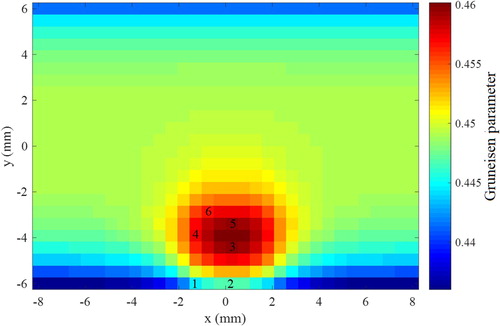
The pressure variations at the locations of the 16 transducers were used to generate the simulated measurements for the inverse analysis, which is aimed at the estimation of the local Gruneisen parameter, either with the Total Variation (TV) prior or with the Gaussian Markov Random Field (GMRF) prior, as described above. The simulated measurements were generated with a frequency of 40.3 MHz. Measurement errors were Gaussian, additive, uncorrelated, with zero mean and a standard deviation of 3% of the exact pressure values. In order to avoid an inverse crime, the Gruneisen parameter was estimated in a mesh much coarser than that used to generate the simulated measurements, with 32 volumes in the x and y directions. The Gruneisen parameter was assumed with local support limited to each finite control volume used for the discretization of the region. The exact values of the Gruneisen parameter on the coarse mesh are shown by Figure 6. Selected volumes that are used to address the accuracy of the inverse problem solution are identified by numbers in Figure 6.

Figure 6. Exact values of Gruneisen parameter on the coarse grid.

For the solution of the inverse problem with the Markov Chain Monte Carlo method, a Gaussian random walk proposal was utilized, with zero mean and a standard deviation of 2 × 10⁻⁴P^(t-1), which resulted in acceptance rates around 26%. The initial states of the Markov chains for the Gruneisen parameter were taken as 0.45 for all positions. For the other model parameters, the chains were started at the mean values of their Gaussian priors, which were centred at the exact values used to generate the simulated measurements, with a standard deviation of 0.5% of the mean values. Similar Gaussian priors, with a standard deviation of 2% of the mean values, were also used for the Gruneisen parameter for deep positions (y > 2 mm), since the focus of this work is the region of the tumour that is heated to larger temperatures. The hyperparameter for the case with Total Variation prior was fixed as γ = 8 × 10⁻⁴, based on numerical tests. For the Gaussian Markov Random Field prior, the Rayleigh hyperprior for γ (see equation 17) was centred at γ₀ = 8 × 10⁻⁴.

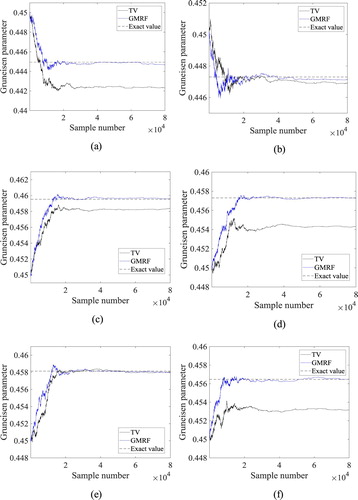
The Markov chains for the Gruneisen parameter with 8 × 10⁴ states, obtained with the Total Variation and Gaussian Markov Random Field priors, at the volumes 1, 2, 3, 4, 5 and 6 (see Figure 6) are presented by Figures 7(a-f), respectively. These volumes were selected because they are located in the region of most interest for the temperature estimation, that is, inside and around the tumour. Figures 7(a-f) indicate that more accurate results were obtained with the use of the Gaussian Markov Random Field prior. Note in Figures 7(a, c, d and f) that the chains generated with the Total Variation prior did not reach equilibrium around the exact values of the Gruneisen parameter for volumes 1, 3, 4 and 6, respectively. On the other hand, the chains generated with the Gaussian Markov Random Field prior reached equilibrium around values much closer to the exact ones than the chains generated with the Total Variation prior, at all volumes.

Figure 7. Markov chains for the Gruneisen parameter at selected volumes: (a) Volume 1; (b) Volume 2; (c) Volume 3; (d) Volume 4; (e) Volume 5; (f) Volume 6.

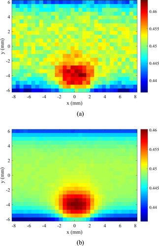
The last 4 × 10⁴ states of the chains were used for the computation of the statistics presented below, when equilibrium could be assured for all volumes. As a representative example, the histograms of these last 4 × 10⁴ states of the chains for volume 5 (see Figure 6) are presented by Figure 8, for both the Total Variation and the Gaussian Markov Random Field priors. The histogram obtained with the Gaussian Markov Random Field prior exhibits variance smaller than that obtained with the Total Variation prior and includes the exact value of the Gruneisen parameter (0.458). The Total Variation prior is more suitable for situations where sharp gradients must be preserved, while the Gaussian Markov Random Field prior is more suitable for cases where a smooth inverse problem solution is sought [38], like in the present case. The local variation (means of the equilibrium states of the Markov chains) of the Gruneisen parameters estimated with TV and GMRF priors are presented by Figures 9(a and b), respectively. These figures show that the Gruneisen parameter estimated with the GMRF prior is smoother and in better agreement with the exact one (see also Figure 6) than that estimated with the TV prior. Moreover, since the normalizing constant for the Gaussian Markov Random Field prior is analytically known, despite the fact that it represents an unlimited variance, the parameter γ in equation (15) was treated as a hyperparameter and computed with the Rayleigh prior given by equation (17). On the other hand, the normalizing constant for the Total Variation prior is analytically intractable, which required that the parameter γ in equation (13) be fixed by numerical tests. Therefore, we hereafter limit the presentation of the results to cases involving the Gaussian Markov Random Field prior.

Figure 8. Histograms of equilibrium states of the Markov chains in volume 5 obtained with total variation prior and Gaussian Markov Random Field prior.

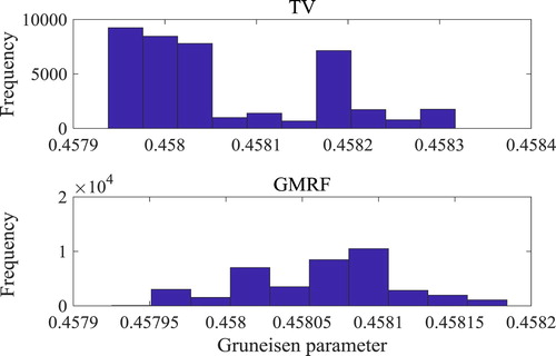
Figure 9. Means of the Gruneisen parameter estimated with: (a) Total Variation prior; (b) Gaussian Markov Random Field prior.

In this work, the experimental data of sound speed, thermal expansion coefficient and specific heat of muscle [37,60–62] were used to relate the Gruneisen parameter to temperature. A linear relation between the Gruneisen parameter for muscle and temperature was obtained, as shown by Figure 10. Such relation is given by [37,60–62]: (18) $T(x,y,t)=115.9\mathrm{\Gamma }(x,y,t)-13$(18)

Figure 10. Variation of the Gruneisen parameter of muscle with temperature [37,60–62].

Equation (18) was used to recover the temperatures from the Gruneisen parameters for each state of the Markov chains. Hence, samples of the local temperature statistical distributions were generated with the samples of the posterior distributions of the Gruneisen parameters, by using equation (18). The estimated local temperatures (means of the samples) were in excellent agreement with the exact temperatures, as shown by Table 2 for the selected volumes (see figure 6). The agreement between the estimated means and the exact temperatures was better than 0.03°C. Table 2 also shows that the uncertainties related to the estimated means, represented by their 99% confidence intervals [40], were smaller than 0.07°C. Although equation (18) was used in this work to relate the Gruneisen parameter to temperature, the procedure advanced in reference [37] can also be used to obtain other equations for different tissues.

Table 2. Estimated temperatures (means of the samples with their associated 99% confidence intervals).

Volume	Exact temperature (°C)	Estimated mean temperature (°C)
1	38.56	38.58 ± 0.002
2	38.82	38.84 ± 0.001
3	40.25	40.27 ± 0.007
4	39.99	40.02 ± 0.003
5	40.24	40.25 ± 0.07
6	39.90	39.93 ± 0.03

Figure 11 presents the estimated means of the local temperatures. A comparison of this figure (obtained in a coarse mesh) with the exact temperatures presented by Figure 2 (obtained with a refined mesh) also reveals that the proposed methodology resulted in accurate estimates of the local temperatures.

Figure 11. Estimated temperatures.

Conclusions

In this work, an inverse method was applied to recover the temperature distribution in a two-dimensional region, by estimating the local variation of the Gruneisen parameter in a photoacoustic problem. A Markov chain Monte Carlo method was used for the inverse problem solution. The Metropolis-Hastings algorithm was implemented to generate samples of the posterior distribution and the solution of the inverse problem was recast as statistical inference over these samples. The samples of the statistical distributions for the local temperatures were based on the Markov chains generated for the Gruneisen parameter. The effects of non-informative priors on the inverse problem solution were examined, by considering a Total Variation prior and a Gaussian Markov Random Field prior.

For the case examined in this paper, a two-dimensional muscle region, which contained a tumour loaded with gold nanorods, was heated by a continuous laser in the near-infrared range, in order to simulate a hyperthermia treatment of cancer. At a specific time, a laser pulse was additionally imposed on the region, for the temperature measurements obtained as the solution of an inverse photoacoustic problem. The simulated measurements of two ultrasound linear array transducers were used for the inverse analysis, which was performed on a mesh much coarser than the one used to generate the simulated measurements, in order to avoid an inverse crime. In general, the local estimated means of the equilibrium Markov chains for the Gruneisen parameter were closer to the exact values when the Gaussian Markov Random Field prior was applied, instead of the Total Variation prior. The present inverse photoacoustic technique resulted in estimated mean temperatures with small 99% confidence intervals. The estimated means were in an agreement better than 0.03°C at selected volumes in the tumour region, despite the use of non-informative priors.

Acknowledgements

The authors are thankful for the support provided by CNPq, CAPES and FAPERJ, Brazilian agencies for the fostering of science. Also, the authors are thankful to Prof. Bradley Treeby who kindly provided a copy of the Matlab toolbox k-Wave.

Disclosure statement

There are no relationships of all authors with any people or organizations that could inappropriately influence (bias) this work.

Additional information

Funding

This work was supported by Conselho Nacional de Desenvolvimento Científico e Tecnológico [Ph.D. Scholarship and Universal Project]; Coordenação de Aperfeiçoamento de Pessoal de Nível Superior [PROEX]; Fundação Carlos Chagas Filho de Amparo à Pesquisa do Estado do Rio de Janeiro [Ph.D. schollarship and Cientista do Estado award].

References

- Nicandro C-R, Efrén M-M, María Yaneli A-A, et al. Evaluation of the diagnostic power of thermography in breast cancer using Bayesian network classifiers. Comput. Math. Methods Med. 2013;2013: 1–10. doi: 10.1155/2013/264246
- Kiskova T, Karasova M, Steffekova Z, et al. Thermography use as a predictive tool in early diagnosis of breast cancer. Adv. Tech. Biol. Med. 2017;5:2379–1764. doi: 10.4172/2379-1764.1000217
- Pouget J-P, Lozza C, Deshayes E, et al. Introduction to radiobiology of targeted radionuclide therapy. Front. Med. 2015;2:428. doi: 10.3389/fmed.2015.00012
- Dewhirst M, Viglianti B, Lora-Michiels M, et al. Thermal dose requirement for tissue effect: experimental and clinical findings. Proc SPIE Int Soc Opt Eng. 2003;4954:37. doi: 10.1117/12.476637
- Stoll AM, Greene LC. Relationship between pain and tissue damage due to thermal radiation. J. Appl. Physiol. 1959;14:373–382. doi: 10.1152/jappl.1959.14.3.373
- Lamien B, Orlande HRB, Eliçabe GE, et al. State estimation problem in hyperthermia treatment of tumors loaded with nanoparticles, in: Proc. 15th Int. Heat Transf. Conf. IHTC 2014, 2014.
- Mcclay EF. Cancer management in man: chemotherapy, biological therapy, hyperthermia and supporting measures. Cancer Manag. Man Chemother. Biol. Ther. Hyperth. Support. Meas. 2011;13:39–60. doi: 10.1007/978-90-481-9704-0
- Field SB, Franconi C. Physics and technology of hyperthermia; 2012. doi: 10.1007/978-94-009-3597-6
- Bermeo Varon LA, Barreto Orlande HR, Eliçabe GE. Estimation of state variables in the hyperthermia therapy of cancer with heating imposed by radiofrequency electromagnetic waves. Int. J. Therm. Sci. 2015;98:228–236. doi: 10.1016/j.ijthermalsci.2015.06.022
- Foster KR, Cheever EA. Microwave radiometry in biomedicine: a reappraisal. Bioelectromagnetics. 1992;13:567–579. doi: 10.1002/bem.2250130611
- Leroy Y, Bocquet B, Mamouni A. Non-invasive microwave radiometry thermometry. Physiol. Meas. 1998;19:127–148. doi: 10.1088/0967-3334/19/2/001
- Edrich J, Jobe WE, Cacak RK, et al. Imaging Thermograms at centimeter and millimeter wavelengths. Ann. N. Y. Acad. Sci. 1980;335:456–474. doi: 10.1111/j.1749-6632.1980.tb50769.x
- De Poorter J, De Wagter C, De Deene Y, et al. Noninvasive MRI thermometry with the proton resonance frequency (PRF) method: in vivo results in human muscle. Magn. Reson. Med. 1995;33:74–81. doi: 10.1002/mrm.1910330111
- Cady EB, D’Souza PC, Penrice J, et al. The estimation of local brain temperature by in vivo 1H magnetic resonance spectroscopy. Magn. Reson. Med. 1995;33:862–867. doi: 10.1002/mrm.1910330620
- Young IR, Hand JW, Oatridge A, et al. Further observations on the measurement of tissue T1 to monitor temperature in vivo by MRI. Magn. Reson. Med. 1994;31:342–345. doi: 10.1002/mrm.1910310317
- Bertsch F, Mattner J, Stehling MK, et al. Non-invasive temperature mapping using MRI: comparison of two methods based on chemical shift and T1-relaxation. Magn. Reson. Imaging. 1998;16:393–403. doi: 10.1016/S0730-725X(97)00311-1
- Delannoy J, Chen CN, Turner R, et al. Noninvasive temperature imaging using diffusion MRI. Magn. Reson. Med. 1991;19:333–339. doi: 10.1002/mrm.1910190224
- Bleier AR, Jolesz FA, Cohen MS, et al. Real-time magnetic resonance imaging of laser heat deposition in tissue. Magn. Reson. Med. 1991;21:132–137. doi: 10.1002/mrm.1910210116
- Germain D, Chevallier P, Laurent A, et al. MR monitoring of tumour thermal therapy. Magn. Reson. Mater. Physics, Biol. Med. 2001;13:47–59. doi:10.1016/S1352-8661(01)00123-5
- Rieke V, Pauly KB, thermometry MR. J. Magn. Reson. Imaging. 2008;27:376–390. doi: 10.1002/jmri.21265
- Seip R, Ebbini ES. Noninvasive estimation of tissue temperature response to heating fields using diagnostic ultrasound. IEEE Trans. Biomed. Eng. 1995;42:828–839. doi: 10.1109/10.398644
- Maass Moreno R, Damianou CA, Sanghvi NT. Noninvasive temperature estimation in tissue via ultrasound echo-shifts. Part II. In vitro study. J. Acoust. Soc. Am. 1996;100:2522–2530. doi: 10.1121/1.417360
- Pulkkinen A, Cox BT, Arridge SR, et al. Quantitative photoacoustic tomography using illuminations from a single direction. J. Biomed. Opt. 2015;20:36015. doi: 10.1117/1.JBO.20.3.036015
- Cox BT, Laufer JG, Beard PC. Quantitative photoacoustic image reconstruction using fluence dependent chromophores. Biomed. Opt. Express. 2010;1:201–208. doi: 10.1364/BOE.1.000201
- Yuan Z, Jiang H. Quantitative photoacoustic tomography: recovery of optical absorption coefficient maps of heterogeneous media. Appl. Phys. Lett. 2006;88:231101. doi: 10.1063/1.2209883
- Ripoll J, Ntziachristos V. Quantitative point source photoacoustic inversion formulas for scattering and absorbing media. Phys. Rev. E - stat. nonlinear. Soft Matter Phys. 2005;71:2331. doi: 10.1103/PhysRevE.71.031912
- Jetzfellner T, Razansky D, Rosenthal A, et al. Performance of iterative optoacoustic tomography with experimental data. Appl. Phys. Lett. 2009;95:013703. doi: 10.1063/1.3167280
- Banerjee B, Bagchi S, Vasu RM, et al. Quantitative photoacoustic tomography from boundary pressure measurements: noniterative recovery of optical absorption coefficient from the reconstructed absorbed energy map. J. Opt. Soc. Am. A. 2008;25:2347–2356. doi: 10.1364/JOSAA.25.002347
- Yin L, Wang Q, Zhang Q, et al. Tomographic imaging of absolute optical absorption coefficient in turbid media using combined photoacoustic and diffusing light measurements. Opt. Lett. 2007;32:2556. doi: 10.1364/OL.32.002556
- Cox BT, Arridge SR, Beard PC. Simultaneous estimation of chromophore concentration and scattering distributions from multiwavelength photoacoustic images. Proc. SPIE 6856, Photons Plus Ultrasound: Imaging and Sensing 2008: The Ninth Conference on Biomedical Thermoacoustics, Optoacoustics, and Acousto-optics, 68560Y; 2008 Feb 28. doi:10.1117/12.762924
- Laufer J, Simpson R, Kohl M, et al. Effect of temperature on the optical properties of ex vivo human dermis and subdermis. Phys. Med. Biol. 1998;43:2479–2489. http://www.ncbi.nlm.nih.gov/pubmed/9755940 doi: 10.1088/0031-9155/43/9/004
- Ke H, Tai S, Wang LV. Photoacoustic thermography of tissue. J. Biomed. Opt. 2014;19:26003), doi: 10.1117/1.JBO.19.2.026003
- Nikitin SM, Khokhlova TD, Pelivanov IM. Temperature dependence of the optoacoustic transformation efficiency in ex vivo tissues for application in monitoring thermal therapies. J. Biomed. Opt. 2012;17:61214), doi: 10.1117/1.JBO.17.6.061214
- Wu X, Sanders JL, Stephens DN, et al. Photoacoustic-imaging-based temperature monitoring for high-intensity focused ultrasound therapy. 38th Annual International Conference of the IEEE Engineering in Medicine and Biology Society; Orlando, FL. IEEE; 2016. p. 3235–3238.
- Petrova EV, Motamedi M, Oraevsky AA, et al. In vivo cryoablation of prostate tissue with temperature monitoring by optoacoustic imaging. Photons Plus Ultrasoun Imaging Sens 2016. 2016;9708:1–8. doi: 10.1117/12.2211190
- Yu Liaoa XJ, Dong F, Cui Y. Dual-wavelengths photoacoustic temperature measurement. Proc. SPIE. 2017;10256:102561K–1. doi: 10.1117/12.2256956
- Alaeian M, Orlande HRB. Inverse photoacoustic technique for parameter and temperature estimation in tissues. Heat Transf. Eng. 2017;38:1573–1594. doi: 10.1080/01457632.2016.1262721
- Kaipio J, Somersalo E. Statistical and computational inverse problems; 2005. doi: 10.1007/b138659
- Kaipio JP, Fox C. The Bayesian framework for inverse problems in heat transfer. Heat Transf. Eng. 2011;32:718–753. doi: 10.1080/01457632.2011.525137
- Fox C, Nicholls GK, Tan SM. An introduction To inverse problems An introduction To inverse problems. Stat. Ber. 2010: 1–65. doi: 10.1007/978-3-642-32557-1
- Metropolis N, Rosenbluth AW, Rosenbluth MN, et al. Equation of state calculations by fast computing machines. J. Chem. Phys. 1953;21:1087–1092. doi: 10.1063/1.1699114
- Welch AJ, Van Gemert MJC. Optical-thermal response of laser-irradiated tissue; 2011. doi: 10.1007/978-90-481-8831-4
- Paltauf G, Dyer PE. Photomechanical processes and effects in ablation. Chem. Rev. 2003;103:487–518. doi: 10.1021/cr010436c
- Yao D-K, Zhang C, Maslov K, et al. Photoacoustic measurement of the Grüneisen parameter of tissue. J. Biomed. Opt. 2014;19:17007-1–17007–7. doi: 10.1117/1
- Treeby BE, Cox BT. k-Wave: MATLAB toolbox for the simulation and reconstruction of photoacoustic wave fields. J. Biomed. Opt. 2010;15:21314. doi: 10.1117/1.3360308
- Cox BT, Kara S, Arridge SR, et al. k-space propagation models for acoustically heterogeneous media: application to biomedical photoacoustics. J. Acoust. Soc. Am. 2007;121:3453. doi: 10.1121/1.2717409
- Yuan X, Borup D, Wiskin J, et al. Simulation of acoustic wave propagation in dispersive media with relaxation losses by using FDTD method with PML absorbing boundary condition. IEEE Trans. Ultrason. Ferroelectr. Freq. Control. 1999;46:14–23. doi: 10.1109/58.741419
- Lamien B, Orlande HRB, Eliçabe GE. Particle filter and approximation error model for state estimation in hyperthermia. J. Heat Transfer. 2017;139:1–12. doi: 10.1115/1.4034064
- Lamien B, Orlande HRB, Eliçabe GE. Inverse problem in the hyperthermia therapy of cancer with laser heating and plasmonic nanoparticles. Inverse Probl. Sci. Eng. 2017;25:608–631. doi: 10.1080/17415977.2016.1178260
- Star WM. Diffusion theory of light transport, In: Opt. response laser-irradiated tissue; 2011. p. 145–201. doi: 10.1007/978-90-481-8831-4_6
- Carp SA, Prahl SA, Venugopalan V. Radiative transport in the delta-P1 approximation: accuracy of fluence rate and optical penetration depth predictions in turbid semi-infinite media. J. Biomed. Opt. 2004;9:632–647. doi: 10.1117/1.1695412
- Pennes HH. Analysis of tissue and arterial blood temperatures in the resting human forearm 1948. J. Appl. Physiol. 1998;85:5–34. doi: 9714612
- Aykroyd RG. Bayesian estimation for homogeneous and inhomogeneous Gaussian random fields. IEEE Trans. Pattern Anal. Mach. Intell. 1998;20:533–539. doi: 10.1109/34.682182
- Rue H. Gaussian Markov random fields: theory and applications, hand. 104; 2005. 263 p. doi: 10.1007/s00184-007-0162-3
- Anderson JD. Computational fluid dynamics, 1995. doi: 10.1007/978-3-540-85056-4
- Duck FA. Physical properties of tissues. Phys. Prop. Tissues. 1990;336:73–135. doi: 10.1016/B978-0-12-222800-1.50008-5
- Nilsson AMK, Berg R, Andersson-Engels S. Measurements of the optical properties of tissue in conjunction with photodynamic therapy. Appl. Opt. 1995;34:4609–4619. doi: 10.1364/AO.34.004609
- Jain PK, Lee KS, El-Sayed IH, et al. Calculated absorption and scattering properties of gold nanoparticles of different size, shape, and composition: applications in biological imaging and biomedicine. J. Phys. Chem. B. 2006;110:7238–7248. doi: 10.1021/jp057170o
- Tabei M, Mast TD, Waag RC. A k-space method for coupled first-order acoustic propagation equations. J. Acoust. Soc. Am. 2002;111:53–63. doi: 10.1121/1.1421344
- Haney WD, O’Brian MJ. Temperature dependency of ultrasonic propagation properties in biological materials. Tissue Charact. with Ultrasound. 1986: 15–55. http://www.brl.uiuc.edu/Publications/1986/Haney-CRCpress-15-1986.pdf
- Jarvis HFT. The thermal variation of the density of beef and the determination of its coefficient of cubical expansion. Int. J. Food Sci. Technol. 1971;6:383–391. doi: 10.1111/j.1365-2621.1971.tb01625.x
- Varzakas T, Tzia C. Food engineering handbook; 2015. 600. doi: 10.1201/b17843