Structural dynamics model updating with interval uncertainty based on response surface model and sensitivity analysis

ABSTRACT

The uncertainties widely exist in the engineering structures. Though great progress has been made in the study of the finite element (FE) modelling and updating with uncertainty, most model updating methods with uncertainty still suffer from the complexity of implementation. A novel FE model updating method in the structural dynamics with uncertainty is proposed in the paper. The model updating with interval uncertainty consists of two steps. In step one, the response surface model (RSM) between the natural frequency and the updating parameters is constructed according to the quadratic polynomial, and the interval average value of uncertain parameters is identified based on an optimal algorithm and the adaptive response surface model. Then, The half width of interval parameter is identified by combining the RSM and the sensitivity analysis in step two. A significant advantage of the proposed method is that it makes the interval model updating to be understood and implemented in the engineering application more easily. Finally, the proposed method is validated in a two degree-of-freedom mass-spring system and a transport mirror system. The updating results evidently demonstrate the feasibility and reliability of this method.

KEYWORDS:

• Response surface model
• uncertainty
• model updating
• sensitivity analysis
• kernel density estimation

2010 MSC SUBJECT CLASSIFICATION:

• 74H4545

1. Introduction

In the design of practical engineering structures, finite element (FE) models are most often used to simulate the behaviour of real systems. Then, the reliable dynamic model is very important for structural design. However, due to the lack of knowledge or other restrictions, the FE models are the approximations of real world phenomena based on various assumptions, which may detract from the quality and accuracy of simulation results. In order to improve the accuracy of FE simulations to serve the structural design better, the FE model updating techniques are needed to be developed. In the past few decades, various kinds of FE model updating methods have been widely investigated based on the actually observed behaviours of the system. Additionally, experimental modal and vibration data are often used to identify the updating parameters in the field of structural mechanics [1–6].

In most model updating methods, the simulations are usually deterministic where each of the updating parameters is considered to have one ‘true’ value, and the purpose of the updating process is to provide a deterministic estimation on the updating parameters. In reality, there are always uncertainties in nominally identical structures, such as the structural parameter uncertainty (physical material properties, geometric parameters), the assembly joints uncertainty, and the experiment uncertainty (measurement noise, modal identification techniques) et al. As a result, the FE model updating methods with uncertainty have received great attention recently. Recent studies have shown that the simulation results are more reliable when the uncertainties are taken into account [7], suggesting that it is necessary to consider the uncertainties during modelling [8].

In FE model updating with uncertainty, the updated parameters are no longer deterministic and are described as random variables. Usually, the FE model updating methods with uncertainty can be classified into two major categories: probabilistic and non-probabilistic methods. In non-probabilistic methods, the interval method has been intensively investigated. In the earlier works, a probabilistic method proposed by Friswell [9] incorporated the measurement noise into model updating. Subsequently, Bayesian statistical frameworks were adopted to estimate the posterior probabilities of uncertain parameters in the structrual FE model and the biological HIV model by Beck et al. [10–11], Kennedy et al. [12] and Wentworth et al. [13]. Recently, the perturbation and sensitivity analysis methods have been employed in stochastic model updating to improve the efficiency by Khodaparast et al. [14–15] and Hua X G et al. [16–17]. The accuracy of the probabilistic methods depends on the estimation of the probability distribution characteristics of the structural parameters and the responses. Lots of experimental data are required to establish an accurate probability distribution function in the probabilistic methods, which makes it difficult to be applied in engineering. By comparison, the experimental samples are not strictly needed in the FE model updating with interval analysis that was proposed by Sao et al. [18], Khodaparast et al. [19], Gabriele et al. [20] and Fang SE et al. [21]. Unlike the traditional algorithms, the current interval model updating approach decomposes the modelling into two deterministic processes. That is, the upper and lower bounds of the parameters are identified separately. Consequently, the optimization difficulty caused by the interval algorithm is avoided. Though several probabilistic and interval model updating methods have been developed, most of them are still complicated for implementation. Hence, it is necessary to construct a two-step updating method based on interval analysis with the feature of easy implementation.

An FE model updating method based on the response surface model (RSM) and sensitivity analysis is developed in the paper. In the proposed method, the FE model updating process is divided into two steps to identify the means and the half widths of interval parameters respectively, which makes the interval model updating to be performed easily. The remainder of this article is organized as follows. In section 2, the general deterministic FE model updating method based on RSM is introduced to identify the mean of the interval parameter. In section 3, the sensitivity-based FE model updating method is presented to identify the radius of interval parameter. In section 4, two examples are provided to validate the accuracy and reliability of the proposed method. Conclusions are presented in section 5.

2. Identifying the mean of interval parameter

The FE model updating problems are inverse problems, as they aim to invert the standard ‘forward’ relationship between input and output variables of a model. The identification of the mean of interval parameter belongs to the deterministic model updating and it aims to find the optimal parameters of a numerical model such that the best possible fit is obtained between the model output and the observed data. Thus, all deterministic FE model updating methods can be employed to determine the mean of updating parameters. The structure FE models of model updating are often constructed by using commercial FE software like ANSYS, ABAQUS and SAP et al. To avoid the expensive cost in the iterative updating method, the RSM based meta-model has emerged as a convenient alternative to the model updating problems. The primary advantages of RSM in the FE model updating are the easy implementation and high efficiency. Moreover, the function relationship between the input parameters and the desired output is clear in the RSM, and this is advantageous to analyse the sensitivity in the next section.

The RSM is a set of mathematical and statistical techniques designed to gain a better understanding of the overall response by design of experiment (DOE) and subsequent analysis of experimental data. The basic procedure to create a response surface that can serve as a surrogate for the FE model, consists of calculating the response features at various sample points in the parameter space and constructing the function model between the inputs and outputs.

As to the choice of the RSM order, it has been found that a second-order RSM is adequate for most engineering problems [22–23]. However, once such adequacy can not be guaranteed, higher-order models should be considered. As a previous study shown the cross items in the quadratic polynomial function have negligible effects on the fitting accuracy [22], the quadratic polynomial form without the cross items is employed in this study as follows: (1) $\begin{array}{rl}y& =b_0+\sum _{i=1}^n{b}_i{x}_i+\sum _{i=1}^n{b}_{ii}{x}_i^2\\ & =b_0+\sum _{i=1}^n{b}_{ii}{\left(x_i+\frac{b_i}{2b_{ii}}\right)}^2-\sum _{i=1}^n\frac{b_i^2}{4b_{ii}}\end{array}$(1) where $b_0$, $b_i$ and $b_{ii}$ are the polynomial coefficients, and n is the number of variables, and $x_i$ is the ith variable. The least-squares method (LSM) of estimation technique is applied to obtain the coefficients by minimizing the error norm defined as (2) $\begin{array}{rl}L& ={\left(y-b_0+\sum _{i=1}^n{b}_i{x}_i+\sum _{i=1}^n{b}_{ii}{x}_i^2\right)}^2\\ & =(y-Xb{)}^T(y-Xb)\end{array}$(2) where X is the vector $\left[\begin{array}{ccc}1& x_i& x_i^2\end{array}\right]$, b is the vector $\left[\begin{array}{ccc}{b}_0& b_i& b_{ii}^{}\end{array}\right]$.

The least-squares estimate of b is obtained by (3) $b=(X^{T}X{)}^{-1}\left(X^{T}y\right)$(3)

The deterministic model updating consists in determining an optimal set of model parameters as described by (4) $\left\{\begin{array}{c}\begin{array}{cc}Min& F\left(p\right)=\end{array}max\left(∥\frac{y_e-y_a\left(p\right)}{y_e}∥\right)\\ s.t.\begin{array}{cc}& \underset{\_}{p}\le p\le \overline{p}\end{array}\end{array}\right.$(4) where $p\in R^N$ are the updating parameters, $y_e$ and $y_a\left(p\right)$ are a given set of experiment and simulation data, respectively.

In fact, the estimation of the original intervals of the updating parameters may be far from its base line value, the resulting updating parameters could fall in wide range, the fitting accuracy of the RSM could be undesired, and only the local optimization rather than the global optimization could be reached for the updating parameters because of nonlinearity. In order to solve these issues, the adaptive response surface technique is adopted [24].

As one of the most important artificial intelligence algorithms, the genetic algorithms (GA) can obtain a global minimum solution theoretically and have been employed for structural model updating by many researchers [25]. In this study, it is adopted to identify the mean of interval parameters. The R-square index is used to evaluate the accuracy of a reconstructed RSM beforce the optimization. 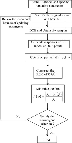In the optimization procedure, the convergent criterion is specified $|F_{k+1}-F_k|/F_k\le {\epsilon }_1$ or $F_k\le {\epsilon }_2$ where ${\epsilon }_1$ and ${\epsilon }_2$ are enough small values. If the optimization result dissatisfies the criterion in the current iteration step, the current values are regarded as the centre of updating parameters in the next iteration step and the new interval and DOE points of updating parameters are specified. Then, calculating the responses of the structure at new sample points, constructing new RSM and identifying the mean of updating parameters are repeated until the convergent criterion is satisfied. The flow chart for the determination of the mean of updating parameters is outlined in Figure 1.

Figure 1. Flow chart identifying the mean of updating parameters.

3. Identifying the radius of interval parameter

Assuming that the updating parameter p is the interval uncertain variable, it can be described by the interval analysis as: (5) $p^I=\left[\begin{array}{cc}\underset{\_}{p}& \overline{p}\end{array}\right]=p^c+\left[\begin{array}{cc}-\mathrm{\Delta }p& \mathrm{\Delta }p\end{array}\right]=p^c+\mathrm{\Delta }{p}^I$(5) where $\underset{\_}{p}$ and $\overline{p}$ are the lower and upper bounds of the interval parameter p, $p^c=0.5\times (\underset{\_}{p}+\overline{p})$ is the mean of the interval parameter p, $\mathrm{\Delta }p=0.5\times (\overline{p}-\underset{\_}{p})$ is the half width of the interval parameter p, that is to say, the radius of the interval parameter p, $\mathrm{\Delta }{p}^I=\left[\begin{array}{cc}-\mathrm{\Delta }p& \mathrm{\Delta }p\end{array}\right]$ is the interval expression with the radius $\mathrm{\Delta }p$.

The eigen-frequency $\lambda \left(p\right)$ of the structure with interval uncertain parameter p is also the interval variable. Because the eigen-frequency $\lambda \left(p\right)$ is regressed in the quadratic polynomial form in the previous chapter, according to the Taylor expansion, it can be written as: (6) $\lambda \left(p\right)=\lambda (p^c+\mathrm{\Delta }p)=\lambda \left(p^c\right)+\sum _{i=1}^n\left(\frac{\mathrm{\partial }\lambda \left(p^c\right)}{\mathrm{\partial }{p}_i}\mathrm{\Delta }{p}_i+\frac{1}{2}\cdot \frac{{\mathrm{\partial }}^{\mathrm{\prime \prime }}\lambda \left(p^c\right)}{\mathrm{\partial }{p^{\mathrm{\prime \prime }}}_i}\mathrm{\Delta }{p}_i^2\right)$(6) By applying the interval extension theory [26] to Equation (6), the bounds and radius of $\lambda \left(p\right)$ can be written as: (7a) $\overline{\lambda }=\lambda \left(p^c\right)+\sum _{i=1}^n\left|\frac{\mathrm{\partial }\lambda \left(p^c\right)}{\mathrm{\partial }{p}_i}+\frac{1}{2}\cdot \frac{{\mathrm{\partial }}^{\mathrm{\prime \prime }}\lambda \left(p^c\right)}{\mathrm{\partial }{p^{\mathrm{\prime \prime }}}_i}\mathrm{\Delta }{p}_i\right|\mathrm{\Delta }{p}_i$(7a) (7b) $\underset{\_}{\lambda }=\lambda \left(p^c\right)-\sum _{i=1}^n\left|\frac{\mathrm{\partial }\lambda \left(p^c\right)}{\mathrm{\partial }{p}_i}+\frac{1}{2}\cdot \frac{{\mathrm{\partial }}^{\mathrm{\prime \prime }}\lambda \left(p^c\right)}{\mathrm{\partial }{p^{\mathrm{\prime \prime }}}_i}\mathrm{\Delta }{p}_i\right|\mathrm{\Delta }{p}_i$(7b) (7c) $\mathrm{\Delta }{\lambda }^I=\left[\begin{array}{cc}-\sum _{i=1}^n\left|\frac{\mathrm{\partial }\lambda \left(p^c\right)}{\mathrm{\partial }{p}_i}+\frac{1}{2}\cdot \frac{{\mathrm{\partial }}^{\mathrm{\prime \prime }}\lambda \left(p^c\right)}{\mathrm{\partial }{p^{\mathrm{\prime \prime }}}_i}\mathrm{\Delta }{p}_i\right|\mathrm{\Delta }{p}_i& \sum _{i=1}^n\left|\frac{\mathrm{\partial }\lambda \left(p^c\right)}{\mathrm{\partial }{p}_i}+\frac{1}{2}\cdot \frac{{\mathrm{\partial }}^{\mathrm{\prime \prime }}\lambda \left(p^c\right)}{\mathrm{\partial }{p^{\mathrm{\prime \prime }}}_i}\mathrm{\Delta }{p}_i\right|\mathrm{\Delta }{p}_i\end{array}\right]$(7c)

A sensitivity-based FE model updating method is proposed to identify the updating parameter. The corresponding problem can be written as: (8) $y_e-y_{a\mathrm{\_}j}=S_j(p_{j+1}-p_j)$(8) where $S_j=\mathrm{\partial }{y}_{a\mathrm{\_}j}/\mathrm{\partial }{p}_j$ is the sensitivity matrix of modal parameters that can be obtained by Equation (1).

Assuming that the experimental data and updating parameters are interval variables, the variables in Equation (8) can be determined by the interval method: (9) $\left\{\begin{array}{c}{p}_j=p_j^c+\mathrm{\Delta }{p}_j^I\\ y_e=y_e^c+\mathrm{\Delta }{y}_e^I\\ y_{a\mathrm{\_}j}=y_{a\mathrm{\_}j}^c+\mathrm{\Delta }{y}_{a\mathrm{\_}j}^I\\ S_j=S_j^c+\mathrm{\Delta }{S}_j^I\end{array}\right.$(9) where $y_{a\mathrm{\_}j}^c$ and $S_j^c$ are the modal parameters and the sensitivity matrix when the updating parameters are the means. Since the means of updating parameters are calculated in the previous model updating, $y_{a\mathrm{\_}j}^c$ and $S_j^c$ are considered as constant temporarily. By applying the interval extension theory, $\mathrm{\Delta }{y}_{a\mathrm{\_}j}^I$ and $\mathrm{\Delta }{S}_j^I$ can be written as: (10) $\begin{array}{rl}\mathrm{\Delta }{y}_{a\mathrm{\_}j}^I& =\left[-\sum _{i=1}^n\left|\frac{\mathrm{\partial }{y}_{a\mathrm{\_}j}\left(p^c\right)}{\mathrm{\partial }{p}_i}+\frac{1}{2}\cdot \frac{{\mathrm{\partial }}^{\mathrm{\prime \prime }}{y}_{a\mathrm{\_}j}\left(p^c\right)}{\mathrm{\partial }{p}_i^{\mathrm{\prime \prime }}}\mathrm{\Delta }{p}_i\right|\mathrm{\Delta }{p}_i\right.\\ & \left.\sum _{i=1}^n\left|\frac{\mathrm{\partial }{y}_{a\mathrm{\_}j}\left(p^c\right)}{\mathrm{\partial }{p}_i}+\frac{1}{2}\cdot \frac{{\mathrm{\partial }}^{\mathrm{\prime \prime }}{y}_{a\mathrm{\_}j}\left(p^c\right)}{\mathrm{\partial }{p}_i^{\mathrm{\prime \prime }}}\mathrm{\Delta }{p}_i\right|\mathrm{\Delta }{p}_i\right]\end{array}$(10) (11) $\mathrm{\Delta }{S}_j^I=\left[\begin{array}{cc}-\sum _{i=1}^n\left|\frac{\mathrm{\partial }{S}_j\left(p^c\right)}{\mathrm{\partial }{p}_i}+\frac{1}{2}\cdot \frac{{\mathrm{\partial }}^{\mathrm{\prime \prime }}{S}_j\left(p^c\right)}{\mathrm{\partial }{p^{\mathrm{\prime \prime }}}_i}\mathrm{\Delta }{p}_i\right|\mathrm{\Delta }{p}_i& \sum _{i=1}^n\left|\frac{\mathrm{\partial }{S}_j\left(p^c\right)}{\mathrm{\partial }{p}_i}+\frac{1}{2}\cdot \frac{{\mathrm{\partial }}^{\mathrm{\prime \prime }}{S}_j\left(p^c\right)}{\mathrm{\partial }{p^{\mathrm{\prime \prime }}}_i}\mathrm{\Delta }{p}_i\right|\mathrm{\Delta }{p}_i\end{array}\right]$(11) Substituting Equation (9) into Equation (8), the equation is written as: (12) $y_e^c+\mathrm{\Delta }{y}_e^I-(y_{a\mathrm{\_}j}^c+\mathrm{\Delta }{y}_{a\mathrm{\_}j}^I)=(S_j^c+\mathrm{\Delta }{S}_j^I)(p_{j+1}^c+\mathrm{\Delta }{p}_{j+1}^I-p_j^c-\mathrm{\Delta }{p}_j^I)$(12)

From Equation (12), the zero-order and first-order terms can be separated and consequently we obtain (13) $\mathrm{\Delta }{y}_e^I-\mathrm{\Delta }{y}_{a\mathrm{\_}j}^I=S_j^c(\mathrm{\Delta }{p}_{j+1}^I-\mathrm{\Delta }{p}_j^I)$(13)

The radius of the updating interval parameter p at the jth iteration step can be determined by (14) $\mathrm{\Delta }{p}_{j+1}^I=G_j^c(\mathrm{\Delta }{y}_e^I-\mathrm{\Delta }{y}_{a\mathrm{\_}j}^I)+\mathrm{\Delta }{p}_j^I$(14) where $G_j^c=(S_j^{cT}{S}_j^c{)}^{-1}{S}_j^{cT}$.

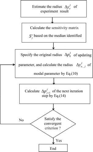
Based on the analysis above, the flow chart identifying the radius of the updating interval parameters is illustrated in Figure 2.

Figure 2. Flow chart identifying the radius of updating parameters.

In practical model updating, the measured data are only a few samples in general. Reasonable interval estimation on experimental data is the precondition to obtain the reliable updated FE model. However, the kernel density estimation (KDE) allows for the capture of the observed distributional structure for the random variables, without having to assume a particular parametric distributional form. Generally speaking, it is a non-parametric method to estimate the interval of parameter [27]. Because of the above features, a non-parametric KDE method is used to estimate the interval of experimental data in this study.

The empirical cumulative distribution function (CDF) and 95% confidence interval (CI) $\left[\begin{array}{cc}{y}_{e\mathrm{\_}95}^{-}& y_{e\mathrm{\_}95}^{+}\end{array}\right]$ of the experimental data can be obtained based on KDE in Matlab easily. As a result, the mean and radius of the experimental data can be obtained by (15a) $y_e^c=0.5\times (y_{e\mathrm{\_}95}^{-}+y_{e\mathrm{\_}95}^{+})$(15a) (15b) $\mathrm{\Delta }{y}_e=0.5\times (y_{e\mathrm{\_}95}^{+}-y_{e\mathrm{\_}95}^{-})$(15b)

4. Case studies

4.1. Example 1: a two degree-of-freedom mass-spring system

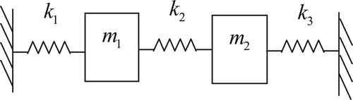
A two degree-of-freedom mass-spring system is shown in Figure 3. The deterministic parameters in the system are $m_1=m_2=1$ kg and $k_1=1$ N/m. The uncertain interval parameters are $k_2=\left[\begin{array}{cc}0.8& 1.2\end{array}\right]$ N/m and $k_3=\left[\begin{array}{cc}0.9& 1.1\end{array}\right]$ N/m.

Figure 3. Two degree-of-freedom mass-spring system.

For simplicity, it is assumed that the uncertain parameters are uniformly distributed. To create such kind of uncertainty, the Latin Hypercube Sample (LHS) method is used to create twenty experimental samples. Afterwards, the experimental results of the first two natural frequencies are obtained according to the samples. Considering the effect of the small sample, the 95% CI of experimental results are estimated by KDE, which is regarded as the interval of experiment results. And then the mean and radius of the experiment results are calculated by Equation (15). The means of the natural frequencies f₁ and f₂ are 0.9993 and 1.7313 rad s⁻¹, respectively. Additionally, the radii of the natural frequencies f₁ and f₂ are 0.0332 and 0.1570 rad s⁻¹, respectively.

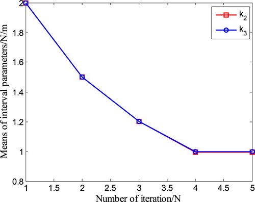
Assuming that the original intervals of k₂ and k₃ are the same as [1.5 2.5], their means are identified according to the optimization course described in Figure 1. The R-square values of all reconstructed RSMs in the optimization procedure are greater than 0.998, which shows that the RSMs have a better accuracy. The convergence curves of k₂ and k₃ are shown in Figure 4 where the optimization is convergent after five iteration steps and the identified means of k₂ and k₃ are 0.9995 and 0.9973 N/m, respectively.

Figure 4. Convergence curves of the means of updating parameters.

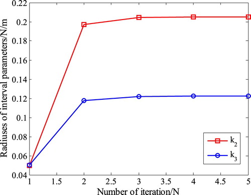
The radii of k₂ and k₃ are calculated according to the optimization course illustrated in Figure 2. The convergence curves of k₂ and k₃ are presented in Figure 5 where the optimization is convergent after five iteration steps and the identified radii of k₂ and k₃ are 0.2051 and 0.1224 N/m, respectively.

Figure 5. Convergence curves of the radiuses of updating parameters.

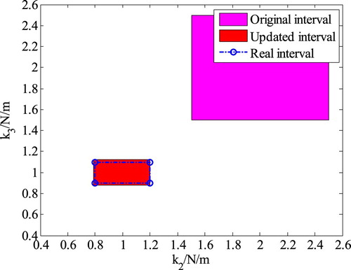
Then, the updated intervals of k₂ and k₃ are [0.7944 1.2046] N/m and [0.8749 1.1197] N/m. The comparison between the original uncertain interval and the updated interval is shown in Figure 6, which shows that the updated interval covers the real interval of updating parameters better. Since the small sample of the experimental data is considered in the model updating process, the updated interval is bigger than the real interval.

Figure 6. Comparison between the original and updated interval of updating parameters.

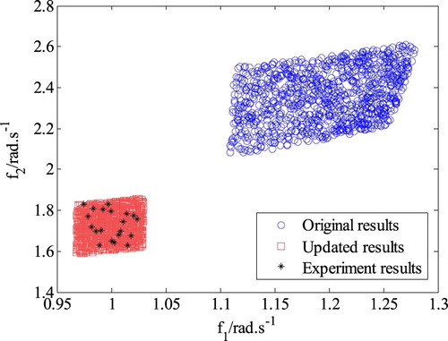
1000 samples of uncertain parameters are created by the LHS according to the original and updated interval and the first two frequencies of the system are calculated. The scatter map of the calculating results and the experimental results shown in Figure 7 indicates that the frequencies of the updated model cover the experimental results better.

Figuer 7. Comparison of frequency between the simulation and experiment results.

4.2. Example 2: transport mirror system

The ShenGuangIII (SGIII) facility is designed for inertial confinement fusion (ICF) high energy experiments with 48 laser beams exactly transported and oriented to target. There are 276 transport mirror systems in the facility, and the dynamic response under ambient vibration is a key factor to affect the stability of the SGIII facility [28]. A classic transport mirror system is shown in Figure 8, which consists of a mirror component and a support frame.

Figure 8. Sketch map of the transport mirror system.

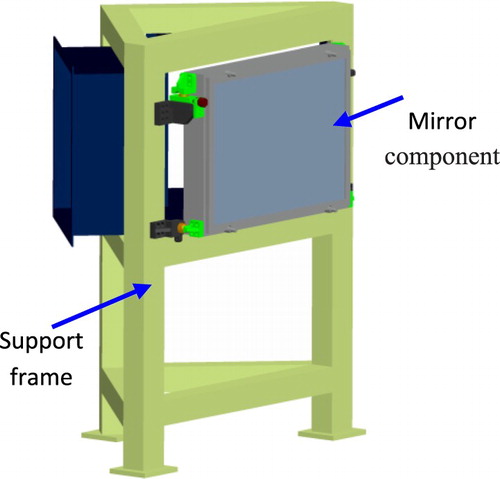
The material of the support frame is steel with the nominal Young’s modulus 200 Gpa, the nominal Poisson’s ratio 0.3 and the nominal density 7850 kg/m³. The material of the mirror is K9 class with the nominal Young’s modulus 80 Gpa, the nominal Poisson’s ratio 0.21 and the nominal density 2510 kg/m³. The transport mirror system is 1.32 m high.

The uncertainty exists in the transport mirror system because of the installation fluctuation and the welding technology fluctuation about the support frame, which the uncertainty of the vibrational characteristics. In order to study how these uncertain factors affect the natural frequencies of the transport mirror system, ten repeated modal experiments were done on the ten same transport mirror systems exactly. Three natural frequencies in the interesting frequency range were found to significantly influence the response of the transport mirror system under the work condition. Then, the first three natural frequencies of the transport mirror system should be updated before the response is calculated. The corresponding natural frequencies were obtained by the modal experiments, as listed in Table 1.

Table 1. Experiment samples of the natural frequencies.

Case	1	2	3	4	5	6	7	8	9	10
f1/Hz	21.573	21.642	21.675	21.472	21.583	21.683	21.657	21.797	21.644	21.462
f2/Hz	22.213	22.223	22.31	22.087	22.168	22.293	22.283	22.407	22.232	22.121
f3/Hz	41.328	41.432	41.58	41.203	41.416	41.56	41.557	41.807	41.497	41.237

Generally, the bolts are ignored in the structural dynamic analysis model generally, the FE model of the cylinder is built by the SOLID185 and SHELL181 element in ANSYS, which is shown in Figure 9. The boundary condition is fully restricted in the bottom of the support frame. The first three calculated modal shapes are shown in Figure 10.

Figure 9. FE model of transport mirror system.

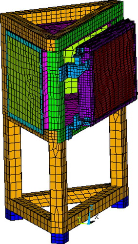
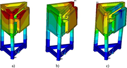
Figure 10. Calculated modal shapes of transport mirror system. (a) first-order mode (b) second-order mode (c) third order mode.

Theoretical analysis finds that the installation uncertainty of the transport mirror system can be characterized by Young’s modulus E₁ of the bottom part of the support frame. The weld uncertainty of the support frame can be characterized by Young’s modulus E₂ of the upper part of the support frame. The goal of FE model updating is to identify the interval between E₁ and E₂.

The weld and the installation on the support frame make its stiffness to reduce, and the installation makes the stiffness to reduce more. Then, assuming that the original intervals of E₁ and E₂ are [1.0 1.5] × 10¹¹ Pa and [1.8 2.0] × 10¹¹ Pa, respectively. Firstly, the means of the first three modal frequencies are estimated by combining the KDE with Equation (15a) according to the experimental data in Table 1. Then, according to the optimal procedure on means of interval parameters in Figure 1, the means of E₁ and E₂ are identified. The R-square values of all reconstructed RSM in the optimization procedure are greater than 0.999, which shows that the RSMs have a better accuracy.

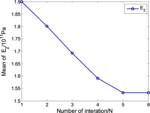
The convergence curves of E₁ and E₂ are shown in Figures 11 and 12, respectively, which shows that the optimization is convergent after six iteration steps.

Figure 11. Convergence curve of the mean of E_1.

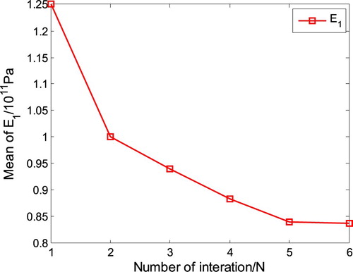
Figure 12. Convergence curve of the mean of E_2.

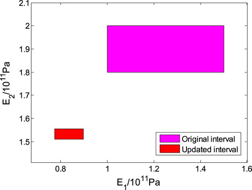
Secondly, the radii of the first three modal frequencies are estimated by combining the KDE with Equation (15b) according to the experimental data in Table 1, they are 0.211, 0.212 and 0.392 Hz, respectively. According to the optimal procedure on radii of interval parameters shown in Figure 2, the radii of E₁ and E₂ are determined. The convergence curves of E₁ and E₂ are shown in Figures 13 and 14, which shows that the optimization is convergent after six iteration steps. The comparison between the original uncertain interval and the updated interval uncertain parameters is shown in Figure 15. The updated results show that Young’s modulus of the bottom part is much less than its nominal value because the simulation boundary is more enhanced than the fact boundary.

Figure 13. Convergence curve of the radius of E_1.

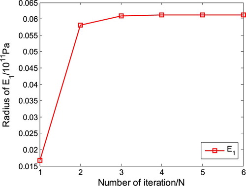
Figure 14. Convergence curve of the radius of E_2.

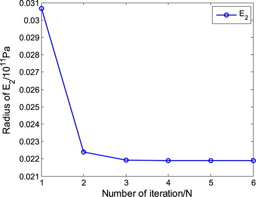
Figure 15. Comparison between the original and the updated interval of uncertain parameters.

In order to validate the optimization results on the interval parameters, 1000 samples of E₁ and E₂ are created by the LHS according to the original and updated intervals, and the first three frequencies of the transport mirror system are calculated by the final RSMs. The scatter map of the calculated results and the experimental results are shown in Figure 16. Furthermore, the 95% CI of the first three natural frequencies of the transport mirror system is calculated according to the 1000 samples, which are regarded as the original and updated interval of the first three natural frequencies, and the comparison on the first three natural frequencies are listed in Table 2. Comparison of the results in Figure 16 and Table 2 show that the natural frequencies of the updated model agree with the experimental results better. It can be seen from Table 2 and Figure 16 that the frequencies of the updated model agree with the experimental results better, and the mean errors of frequencies decrease from the initial [8.60 11.31]% to [0.26 0.24]%.

Figure 16. Scatter map of the first three natural frequencies.

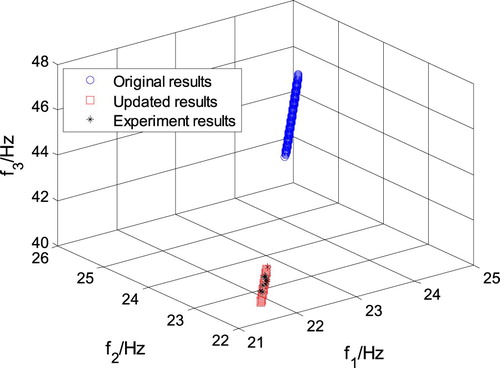
Table 2. Comparison on the natural frequencies between the simulation results and the experimental results.

Mode	Experimental interval/Hz	Original interval/Hz	Error (%)	Updated interval/Hz	Error (%)
1	[21.46 21.80]	[23.39 24.42]	[8.99 12.02]	[21.45 21.79]	[−0.07 −0.04]
2	[22.09 22.41]	[24.05 25.01]	[8.87 11.60]	[22.08 22.42]	[−0.04 0.05]
3	[41.20 41.81]	[44.47 46.12]	[7.94 10.31]	[40.93 41.55]	[−0.66 −0.62]
Mean			[8.60 11.31]		[0.26 0.24]

4.3. Discussions

The time cost in the model updating procedure is mainly to simulate the FE model. In the model updating procedure on the transport mirror system with uncertainty, the FE simulation is only performed in step one. There are nine samples to construct the RSM in each iteration step in example two. We also know that there are six iterations in the example. Then, there are totally 54 times FE simulations on the transport mirror system during updating the model with uncertainty. But, more than hundreds of FE simulations are needed in a determined model updating without the surrogate model, and the number of FE simulations in the model updating with uncertainty are far more than that of a determined model updating. Therefore, the model updating method proposed with interval uncertainty is efficient in the present paper.

5. Conclusions

In summary, an FE model updating method in the structural dynamics with uncertainty is presented. The model updating with interval uncertainty consists of two steps: (1) the means of interval parameters are identified based on the RSMs; (2) and the radii of interval parameters are calculated by combining the RSMs and the sensitivity analysis. The corresponding flows to identify the means and radii of interval parameters are described in detail.

Two examples are used to validate the FE model updating method proposed in the study. The updating results have proved the feasibility and reliability of this method. As the first step of the two-step model updating method with interval uncertain parameters is the classic deterministic FE model updating, most of the deterministic methods can be used instead of the one used in this study, which makes this method user-friendly for other researchers. Besides, the proposed method also estimates the interval of experiment samples by KDE in advance, which confers on this model great prediction power for the dynamic response of structures.

Disclosure statement

No potential conflict of interest was reported by the authors.

Additional information

Funding

This work was supported by Science Challenge Project [grant number TZ2018007], the National Natural Science Foundation of China [grant number 11472256] and the National Key Research and Development Programme of China [grant number 2016YFB0201005].

References

- Mottershead J, Friswell M. Model updating in structural dynamics: a survey. J Sound Vib. 1993;167(2):347–375.
- Fritzen CP, Jennewein D, Kiefer T. Damage detection based on model updating methods. Mech Syst Signal Process. 1998;11(1):163–186.
- Ren R, Beards CF. Identification of ‘effective’ linear joints using coupling and joint identification techniques. ASME J Vib Acoust. 1998;121:331–338.
- Li WL. A new method for structural model updating and joint stiffness identification. Mech Syst Signal Process. 2002;16(1):155–167.
- Bakir PG, Reynders E, Roeck GD. Sensitivity-based finite element model updating using constrained optimization with a trust region algorithm. J Sound Vib. 2007;305:211–225.
- Mottershead J, Link M, Friswell M. The sensitivity method in finite element model updating: a tutorial. Mech Syst Signal Process. 2011;25:2275–2296.
- Oberkampf WL, Roy CJ. Verification and validation in scientific computing. Cambridge: Cambridge University Press; 2010.
- Simoen E, De Roeck G, Lombaert G. Dealing with uncertainty in model updating for damage assessment: a review. Mech Syst Signal Process. 2015: 56–57: 123–149.
- Friswell M. The adjustment of structural parameters using a minimum variance estimator. Mech Syst Signal Process. 1989;3(2):143–155.
- Beck JL, Katafygiotis LS. Updating models and their uncertainties I: Bayesian statistical framework. J Eng Mech. 1998;124(4):455–461.
- Beck JL, Au SK. Bayesian updating of structural models and reliability using Markov chain Monte Carlo simulation. J Eng Mech. 2002;128(4):380–391.
- Kennedy MC, Hagan AO. Bayesian calibration of computer models. J Roy Stat Soc Ser B-Stat Methodol. 2001;63(3):425–464.
- Wentworth MT, Smith RC, Williams B. Bayesian model calibration and uncertainty quantification for an HIV model using adaptive Metropolis algorithms. Inverse Prob Sci Eng. 2018;26(2):233–256.
- Khodaparast H, Mottershead J, FrisWell M. Perturbation methods for the estimation of parameter variability in stochastic model updating. Mech Syst Signal Process. 2008;22(8):1751–1773.
- Husain NA, Khodaparast H, Ouyang HH. Parameter selection and stochastic model updating using perturbation methods with parameter weighting matrix assignment. Mech Syst Signal Process. 2012;32:135–152.
- Hua X G, Ni Y Q, Chen Z Q, et al. An improved perturbation method for stochastic finite element model updating. Int J Numer Methods Eng. 2008;73(13):1845–1864.
- Hua X G, Wen Q, Ni Y Q, et al. Assessment of stochastically updated finite element models using reliability indicator. Mech Syst Signal Process. 2017;82:217–229.
- Rao S S, Berke L. Analysis of uncertain structural systems using interval analysis. AIAA J. 1997;35(4):727–735.
- Khodaparast H, Mottershead J, Badcock K. Interval model updating with irreducible uncertainty using the Kriging predictor. Mech Syst Signal Process. 2011;25(4):1204–1226.
- Gabriele S, Valente C. An interval-based technique for FE model updating. Int J Reliab Saf. 2009;3(1–3):79–103.
- Fang SE, Zhang QH, Ren WX. An interval model updating strategy using interval response surface models. Mech Syst Signal Process. 2015: 60–61. : 909–927.
- Fang SE, Perera R. A response surface methodology based damage identification technique. Smart Mater Struct. 2009;18(6):065009.
- Fang SE, Perera R. Damage identification by response surface model updating using D-optimal design. Mech Syst Signal Process. 2011;25(2):717–733.
- Wang GG. Adaptive response surface method using inherited Latin hypercube design points. J Mech Des. 2003;125(2):210–220.
- Friswell MI, Penny JET, Garvey SD. A combined genetic and eigensensitivity algorithm for the location of damage in structures. Comput Struct. 1998;69(5):547–556.
- Moore RE, Kearfott RB, Cloud MJ. Introduction to interval analysis. Philadelphia: Society for Industrial and Applied Mathematics; 2009.
- McFarland J, Mahadevan S. Error and variability characterization in structural dynamics modeling. Comput Methods Appl Mech Eng. 2008;197(29):2621–2631.
- ChenX J, Wang MC, Wu WK, et al. Structural design of beam transport system in SGIII facility target area. Fusion Eng Des. 2014;89(12):3095–3100.