Solution to a three-dimensional axisymmetric inverse electromagnetic casting problem

ABSTRACT

A new method based on topology optimization is proposed for solving a three-dimensional axisymmetric inverse problem regarding the configuration of electric currents used in the electromagnetic casting technique of the metallurgical industry. These electric currents must generate an electromagnetic field such that when certain mass of liquid metal is placed in the field it levitates acquiring a predefined axisymmetric shape. The method proposed is able to obtain a suitable configuration of electric currents, and is very attractive from the computational point of view, since it is based on a sparse convex quadratic programming formulation for which there are very efficient interior-point solution algorithms.

KEYWORDS:

• Electromagnetic casting
• inverse problem
• axisymmetric geometry
• quadratic programming
• free-surface problem

AMS SUBJECT CLASSIFICATIONS:

• 49Q10
• 90C90
• 90C51
• 65K10
• 65R32

1. Introduction

In this paper, we present a numerical method to solve a design problem arising in electromagnetic casting (EMC). The EMC is an industrial process used in the metallurgical industry that allows for heating, shaping and controlling of chemical aggressive hot melts. Its main advantage over the conventional crucible melting is that the molten metal does not come into contact with the crucible wall. This is used in the preparation of very pure specimens [1–3].

The direct three-dimensional electromagnetic casting problem is a free-surface problem that consists of obtaining the equilibrium shape of a bubble of liquid metal levitating inside an electromagnetic field created by known alternating electric currents. Complete numerical models to simulate the direct problem in EMC involve the solution to a PDE system including Maxwell, Navier–Stokes and heat equations [3–15]. One of the most important parameters of the problem considered is the frequency of the imposed alternating current in the inductors. If the frequency is high, then the eddy currents are concentrated in a thin layer near the boundary of the liquid metal. Consequently, the numerical simulation must consider boundary layers with an adapted discretization, which makes the simulation of the direct problem very hard, see, e.g. [16]. However, the penetration of the electromagnetic field into the metal is governed by an induction equation depending on the fluid velocity and the magnetic diffusivity. By increasing the frequency, while keeping the field scale fixed, the magnetic Reynolds number becomes small, and Sneyd and Moffatt [6,7] have shown that we can neglect the velocity term in the calculation of the induced field. Hence, we are faced with a standard problem of field penetration into a solid conductor. This leads to an exponential decay of the field inside the conductor which is known as skin effect. When the frequency is very high, e.g. higher than ${10}^4$ Hz, an asymptotic analysis allows to set limit models where the eddy current are concentrated only on the surface, and we can neglect the motion of the fluid and the penetration of the electromagnetic field into the metal [5–7,17–19]. In the present paper, we consider the classic magnetostatic limit model, which has been widely used to find equilibrium configurations [4–7,17–29]. In the case of high frequencies it is known that this model provides results in good agreement with the experimental data, see [20]. In this model, the electromagnetic forces consist of a magnetic pressure acting on the surface of the liquid metal. The equilibrium shape is characterized by the satisfaction of an expression defined on the surface of the liquid metal which involves the surface tension of the liquid, the gravity forces and the magnetic pressure.

The magnetostatic model is adopted here to study the inverse problem related to the EMC problem. This problem consists of determining a configuration of electric currents such that the surface of the molten metal in equilibrium with the exterior electromagnetic field takes on certain prescribed shape. In other words, a solution of the inverse problem is a configuration of electric currents for which the equilibrium liquid metal surface matches the target shape. The existence of solutions for a general three-dimensional problem has been studied theoretically [28]. However, numerical algorithms for finding solutions have been proposed only for two-dimensional inverse EMC models which do not consider gravity forces. For instance, the problem of finding the best location of concentrated electric currents in single solid-core wires of negligible cross-section area was considered in [30]. Shin et al. [29] studied the same problem and presented a direct approach to obtain the best location and intensity of the electric currents. The more realistic case where the inductors are made of a set of bounded insulated strands was studied in [31,32]. In these papers, the number and topology of the inductors are set in advance. In a later article [33], optimal configurations of electric currents were obtained by considering a heuristic topology optimization method based on the Kohn-Vogelius criterion and the topological derivative concept. The same problem was solved in [34] by using mathematical programming techniques.

In the present paper, we propose a numerical method to find a solution of the three-dimensional axisymmetric inverse EMC problem. This problem is more complex than the two-dimensional one considered in previous papers [30–33], even in the axisymmetric case, since the equilibrium of the liquid metal implies a phenomenon of levitation of the liquid metal in the gravitational field. To the best of our knowledge, this is the first article that proposes a numerical method for this problem. The target shape is assumed to have a smooth closed surface diffeomorphic to the unit sphere. Other cases, e.g. toroidal shapes [25,35], are not considered in this paper.

We consider that the electric currents flow inside inductors that are made up of multiple, individually insulated strands of very small cross-section, and assume that the electric current intensity on each strand is the same. In other words, the electric currents are characterized by a uniform electric current density which, on account of the axisymmetry, is flowing in the azimuthal direction of certain cylindrical coordinate system. Hence, these particular kinds of solutions – that we call 0–1 solutions – define a very simple partition of the exterior space: in one region there is an electric current density of certain fixed magnitude (the region where the inductors are), and in the complementary region where the electric current density is zero.

To solve the inverse problem, we propose a topology optimization approach that is based on a simultaneous analysis and design (SAND) formulation [30,31,36]. Special codes devised for axisymmetric problems that use a variable mesh approach will be used to reduce the computational costs. The objective functional of the formulation is a penalized Kohn-Vogelius-like criterion [33,37], which is devised to provide for regular 0–1 solutions. The solution is regular in the sense that its $L_1$ norm is controlled by the penalty term. We show that the discrete version of the penalized SAND formulation is a convex quadratic programming problem that can be efficiently solved by using interior-point optimization algorithms.

The remaining contents of this paper are organized as follows. Section 2 describes the mathematical model of the EMC problem. Section 3 introduces the inverse EMC problem in the axisymmetric case and describes the SAND topology optimization formulation and the variable mesh approach. Six numerical examples of axisymmetric EMC problems are studied in Section 4. Final remarks are given in Section 5.

2. The direct EMC problem

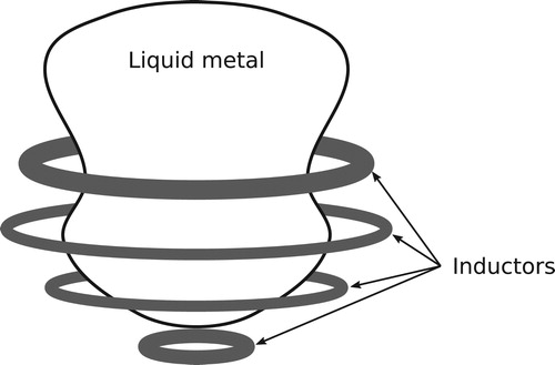
The simplified model of the EMC problem studied here concerns the case of certain mass of liquid metal resting on an electromagnetic field, which is created by alternating electric currents of high frequency flowing in axisymmetric inductors, see Figure 1. We assume that a stationary configuration is reached, see [4,9,21,23,26,38–40] for the physical analysis of the simplifying assumptions.

Figure 1. Electromagnetic casting: liquid metal and circular inductors.

2.1. Mathematical formulation

Let $\mathrm{\Omega }\subset {\mathbb{R}}^3$ be the exterior of the domain ω occupied by the liquid metal, which is assumed closed, simply connected, with a non-void interior and with boundary $\mathrm{\partial }\omega$ of class ${\mathbb{C}}^2$. The equilibrium configurations are characterized by the following equations [24–27,41–43]: (1) $\begin{array}{rl}& {\mathrm{\nabla }}^{\mathrm{\prime }}\times {\mathit{B}}^{\mathrm{\prime }}=\mu {\mathit{J}}^{\mathrm{\prime }}\text{in }{\mathrm{\Omega }}^{\mathrm{\prime }},\end{array}$(1) (2) $\begin{array}{rl}& {\mathrm{\nabla }}^{\mathrm{\prime }}\cdot {\mathit{B}}^{\mathrm{\prime }}=0\text{in }{\mathrm{\Omega }}^{\mathrm{\prime }},\end{array}$(2) (3) $\begin{array}{rl}& {\mathit{B}}^{\mathrm{\prime }}\cdot {\mathit{n}}^{\mathrm{\prime }}=0\text{on }\mathrm{\partial }{\omega }^{\mathrm{\prime }},\end{array}$(3) (4) $\begin{array}{rl}& \parallel {\mathit{B}}^{\mathrm{\prime }}\parallel =O(\parallel x^{\mathrm{\prime }}{\parallel }^{-2})\text{as }\parallel x^{\mathrm{\prime }}\parallel \to \mathrm{\infty },\end{array}$(4) (5) $\begin{array}{rl}& \parallel {\mathit{B}}^{\mathrm{\prime }}{\parallel }^2+{\mathcal{C}}^{\mathrm{\prime }}+x_3^{\mathrm{\prime }}=P^{\mathrm{\prime }}\text{on }\mathrm{\partial }{\omega }^{\mathrm{\prime }}.\end{array}$(5) In Equations (1(1) $\begin{array}{rl}& {\mathrm{\nabla }}^{\mathrm{\prime }}\times {\mathit{B}}^{\mathrm{\prime }}=\mu {\mathit{J}}^{\mathrm{\prime }}\text{in }{\mathrm{\Omega }}^{\mathrm{\prime }},\end{array}$(1) )–(5(5) $\begin{array}{rl}& \parallel {\mathit{B}}^{\mathrm{\prime }}{\parallel }^2+{\mathcal{C}}^{\mathrm{\prime }}+x_3^{\mathrm{\prime }}=P^{\mathrm{\prime }}\text{on }\mathrm{\partial }{\omega }^{\mathrm{\prime }}.\end{array}$(5) ), we used the dimensionless variables $x_i=L{x}_i^{\mathrm{\prime }}$, $\mathcal{C}={\mathcal{C}}^{\mathrm{\prime }}/L$, $\mathit{B}=B_0{\mathit{B}}^{\mathrm{\prime }}$, $\mathit{J}=I{\mathit{J}}^{\mathrm{\prime }}$ and $P=B_0^2/\left(2{\mu }_0\right)P^{\mathrm{\prime }}$, where $L=\sqrt{\sigma /\gamma }$, $B_0=\sqrt{2{\mu }_{0}L\gamma }$, $\mu ={\mu }_{0}IL/B_0$. In these expressions, $\mathit{J}$ is the mean square value of the electric current density vector, which is assumed compactly supported in Ω, $\mathit{B}$ is mean square value of the magnetic-flux density vector, I is a typical value for the current density in the problem considered, ${\mu }_0$ is the vacuum permeability, $\mathit{n}$ is the unit normal vector of $\mathrm{\partial }\omega$ pointing to the liquid metal, $\parallel \cdot \parallel$ denotes the Euclidean norm, $x=(x_1,x_2,x_3)\in {\mathbb{R}}^3$, $\mathcal{C}$ is the mean curvature of $\mathrm{\partial }\omega$ seen from the metal¹, σ and γ are, respectively, the surface tension and the specific weight of the liquid, and the constant P is an unknown to the problem. Physically, P represents the difference between the internal and external pressures at height $x_3=0$. Note the use of the big O notation in Equation (4(4) $\begin{array}{rl}& \parallel {\mathit{B}}^{\mathrm{\prime }}\parallel =O(\parallel x^{\mathrm{\prime }}{\parallel }^{-2})\text{as }\parallel x^{\mathrm{\prime }}\parallel \to \mathrm{\infty },\end{array}$(4) ). Equations (1(1) $\begin{array}{rl}& {\mathrm{\nabla }}^{\mathrm{\prime }}\times {\mathit{B}}^{\mathrm{\prime }}=\mu {\mathit{J}}^{\mathrm{\prime }}\text{in }{\mathrm{\Omega }}^{\mathrm{\prime }},\end{array}$(1) )–(2(2) $\begin{array}{rl}& {\mathrm{\nabla }}^{\mathrm{\prime }}\cdot {\mathit{B}}^{\mathrm{\prime }}=0\text{in }{\mathrm{\Omega }}^{\mathrm{\prime }},\end{array}$(2) ) are the field equations satisfied by the field ${\mathit{B}}^{\prime }$ in the exterior domain. The boundary condition of Equation (3(3) $\begin{array}{rl}& {\mathit{B}}^{\mathrm{\prime }}\cdot {\mathit{n}}^{\mathrm{\prime }}=0\text{on }\mathrm{\partial }{\omega }^{\mathrm{\prime }},\end{array}$(3) ) is a consequence of neglecting the penetration of the magnetic field into the liquid metal. Equation (4(4) $\begin{array}{rl}& \parallel {\mathit{B}}^{\mathrm{\prime }}\parallel =O(\parallel x^{\mathrm{\prime }}{\parallel }^{-2})\text{as }\parallel x^{\mathrm{\prime }}\parallel \to \mathrm{\infty },\end{array}$(4) ) is the growth condition for ${\mathit{B}}^{\prime }$ at infinity, and Equation (5(5) $\begin{array}{rl}& \parallel {\mathit{B}}^{\mathrm{\prime }}{\parallel }^2+{\mathcal{C}}^{\mathrm{\prime }}+x_3^{\mathrm{\prime }}=P^{\mathrm{\prime }}\text{on }\mathrm{\partial }{\omega }^{\mathrm{\prime }}.\end{array}$(5) ) is the equilibrium equation of the liquid metal surface [24,25]. For the sake of simplicity, we drop the prime symbols in the following equations. In the direct (dimensionless) EMC problem μ and the electric current density $\mathit{J}$ are known, and we have to find the shape ω of certain volume V , such that there exist $\mathit{B}\in W^1(\mathrm{\Omega }{)}^3$ and $P\in \mathbb{R}$ satisfying Equations (1(1) $\begin{array}{rl}& {\mathrm{\nabla }}^{\mathrm{\prime }}\times {\mathit{B}}^{\mathrm{\prime }}=\mu {\mathit{J}}^{\mathrm{\prime }}\text{in }{\mathrm{\Omega }}^{\mathrm{\prime }},\end{array}$(1) )–(5(5) $\begin{array}{rl}& \parallel {\mathit{B}}^{\mathrm{\prime }}{\parallel }^2+{\mathcal{C}}^{\mathrm{\prime }}+x_3^{\mathrm{\prime }}=P^{\mathrm{\prime }}\text{on }\mathrm{\partial }{\omega }^{\mathrm{\prime }}.\end{array}$(5) ); where $W^1\left(\mathrm{\Omega }\right)$ is the closure of $D\left(\overline{\mathrm{\Omega }}\right)$ with the semi-norm $u\to \parallel \mathrm{\nabla }u{\parallel }_{L^2\left(\mathrm{\Omega }\right)}$, see [27].

Since Ω is simply connected, then $\mathit{B}={\mathit{B}}_1+\mathrm{\nabla }\varphi$, where ${\mathit{B}}_1$ is a particular solution in ${\mathbb{R}}^3$ of Equations (1(1) $\begin{array}{rl}& {\mathrm{\nabla }}^{\mathrm{\prime }}\times {\mathit{B}}^{\mathrm{\prime }}=\mu {\mathit{J}}^{\mathrm{\prime }}\text{in }{\mathrm{\Omega }}^{\mathrm{\prime }},\end{array}$(1) )–(2(2) $\begin{array}{rl}& {\mathrm{\nabla }}^{\mathrm{\prime }}\cdot {\mathit{B}}^{\mathrm{\prime }}=0\text{in }{\mathrm{\Omega }}^{\mathrm{\prime }},\end{array}$(2) ): (6) ${\mathit{B}}_1\left(x\right)=\frac{\mu }{4\pi }{\int }_{{\mathbb{R}}^3}\frac{\mathit{J}\left(y\right)\times (x-y)}{\parallel x-y{\parallel }^3}\mathrm{d}y,$(6) and ϕ is the unique solution in $W^2\left(\mathrm{\Omega }\right)$ of (7) $\begin{array}{rl}-\mathrm{\Delta }\varphi & =0\text{in }\mathrm{\Omega },\\ \frac{\mathrm{\partial }\varphi }{\mathrm{\partial }\mathit{n}}& =-{\mathit{B}}_1\cdot \mathit{n}\text{on }\mathrm{\partial }\omega ,\\ \parallel \varphi \left(x\right)\parallel & =O(\parallel x{\parallel }^{-1}),\parallel \mathrm{\nabla }\varphi \left(x\right)\parallel =O(\parallel x{\parallel }^{-2})\text{as }\parallel x\parallel \to \mathrm{\infty },\end{array}$(7) where $W^2\left(\mathrm{\Omega }\right)$ is the closure of $D\left(\overline{\mathrm{\Omega }}\right)$ with the semi-norm $u\to \sum _{i,j}\parallel {\mathrm{\partial }}^{2}u/\mathrm{\partial }{x}_i\mathrm{\partial }{x}_j{\parallel }_{L^2\left(\mathrm{\Omega }\right)}$, see [27]. In the case considered, i.e. with $\mathrm{\partial }\omega$ of class ${\mathbb{C}}^2$, the solution ϕ to Equation (7(7) $\begin{array}{rl}-\mathrm{\Delta }\varphi & =0\text{in }\mathrm{\Omega },\\ \frac{\mathrm{\partial }\varphi }{\mathrm{\partial }\mathit{n}}& =-{\mathit{B}}_1\cdot \mathit{n}\text{on }\mathrm{\partial }\omega ,\\ \parallel \varphi \left(x\right)\parallel & =O(\parallel x{\parallel }^{-1}),\parallel \mathrm{\nabla }\varphi \left(x\right)\parallel =O(\parallel x{\parallel }^{-2})\text{as }\parallel x\parallel \to \mathrm{\infty },\end{array}$(7) ) is known to be in ${\mathbb{C}}^1\left(\overline{\mathrm{\Omega }}\right)\cap {\mathbb{C}}^2\left(\mathrm{\Omega }\right)$, see [44]. In addition, the equilibrium equation of the liquid metal surface in terms of ϕ is (8) $\parallel {\mathit{B}}_1+\mathrm{\nabla }\varphi {\parallel }^2+\mathcal{C}+x_3=P\text{on }\mathrm{\partial }\omega .$(8) We note that since $\mathit{J}$ is a divergence-free vector field, the field ${\mathit{B}}_1$ of Equation (6(6) ${\mathit{B}}_1\left(x\right)=\frac{\mu }{4\pi }{\int }_{{\mathbb{R}}^3}\frac{\mathit{J}\left(y\right)\times (x-y)}{\parallel x-y{\parallel }^3}\mathrm{d}y,$(6) ) can be obtained from the vector potential $\mathit{A}$ by [38]: (9) ${\mathit{B}}_1=\mathrm{\nabla }\times \mathit{A},\mathrm{with}\mathit{A}\left(x\right)=\frac{\mu }{4\pi }{\int }_{{\mathbb{R}}^3}\frac{\mathit{J}\left(y\right)}{\parallel x-y\parallel }dy.$(9)

2.2. Axisymmetric problem

In the axisymmetric case the electric current density has only the azimuthal component, i.e. $\mathit{J}\left(x\right)=J_{\theta }(r,z){\mathit{e}}_{\theta }$, where $(r,\theta ,z)$ are the usual cylindrical coordinates of the generic point x, i.e. $x_1=r\cos \left(\theta \right)$, $x_2=r\sin \left(\theta \right)$, and $x_3=z$, while ${\mathit{e}}_r$, ${\mathit{e}}_{\theta }$, and ${\mathit{e}}_z$ are the unit basis vectors corresponding to the radial, azimuthal and vertical directions. Let the sets $\mathcal{R}$ and $\mathcal{D}$ be given by (10) $\mathcal{R}=\left\{\right(r,z)\in {\mathbb{R}}^2:r>0\},\mathcal{D}=\left\{\right(r,z)\in \mathcal{R}:(r,\theta ,z)\in \mathrm{\Omega }\}.$(10) Axisymmetric functions do not depend on the azimuthal coordinate θ. Hence, from now on we will consider x and y as points in $\mathcal{R}$. The following notations will be extensively used in this section: (11) $\begin{array}{r}x=(r_x,z_x),y=(r_y,z_y),\mathrm{\Delta }z=z_x-z_y,\end{array}$(11) (12) $\begin{array}{r}R=\sqrt{\mathrm{\Delta }{z}^2+(r_x+r_y{)}^2},D=\sqrt{\mathrm{\Delta }{z}^2+(r_x-r_y{)}^2},\end{array}$(12) (13) $\begin{array}{r}{\beta }^2=4r_x{r}_y/R,K_{\beta }=K\left({\beta }^2\right),E_{\beta }=E\left({\beta }^2\right),\end{array}$(13) where K and E are the complete elliptic integrals of the first and second kinds, respectively, see [38].

By integrating the expression in Equation (9(9) ${\mathit{B}}_1=\mathrm{\nabla }\times \mathit{A},\mathrm{with}\mathit{A}\left(x\right)=\frac{\mu }{4\pi }{\int }_{{\mathbb{R}}^3}\frac{\mathit{J}\left(y\right)}{\parallel x-y\parallel }dy.$(9) ) in a circular loop of constant $r_y$ and $z_y$, we obtain the vector potential as [38, Section 5.5] (14) $\begin{array}{rl}\mathit{A}\left(x\right)& =A_{\theta }\left(x\right){\mathit{e}}_{\theta }\end{array}$(14) (15) $\begin{array}{rl}\mathrm{with}{A}_{\theta }\left(x\right)& =\frac{\mu }{4\pi }{\int }_{\mathcal{R}}{J}_{\theta }\left(y\right)\frac{R}{r_x}\left[\right(2-{\beta }^2)K_{\beta }-2E_{\beta }]dy,\end{array}$(15) From Equations (9(9) ${\mathit{B}}_1=\mathrm{\nabla }\times \mathit{A},\mathrm{with}\mathit{A}\left(x\right)=\frac{\mu }{4\pi }{\int }_{{\mathbb{R}}^3}\frac{\mathit{J}\left(y\right)}{\parallel x-y\parallel }dy.$(9) ) to (15(15) $\begin{array}{rl}\mathrm{with}{A}_{\theta }\left(x\right)& =\frac{\mu }{4\pi }{\int }_{\mathcal{R}}{J}_{\theta }\left(y\right)\frac{R}{r_x}\left[\right(2-{\beta }^2)K_{\beta }-2E_{\beta }]dy,\end{array}$(15) ) we have (16) $\begin{array}{rl}{\mathit{B}}_1\left(x\right)& =B_r\left(x\right){\mathit{e}}_r+B_z\left(x\right){\mathit{e}}_z\end{array}$(16) (17) $\begin{array}{rl}\mathrm{with}{B}_r\left(x\right)& =\frac{\mu }{4\pi }{\int }_{\mathcal{R}}{J}_{\theta }\left(y\right)\left[-\frac{2\mathrm{\Delta }z}{r_{x}R}(K_{\beta }-E_{\beta })+\frac{4r_y\mathrm{\Delta }z}{RD}{E}_{\beta }\right]\mathrm{d}y,\end{array}$(17) (18) $\begin{array}{rl}{B}_z\left(x\right)& =\frac{\mu }{4\pi }{\int }_{\mathcal{R}}{J}_{\theta }\left(y\right)\left[\frac{1}{R}(2K_{\beta }-E_{\beta })-\frac{R^2-4r_y^2}{RD}{E}_{\beta }\right]\mathrm{d}y.\end{array}$(18) Hence ${\mathit{B}}_1$ is axisymmetric with a zero azimuthal component. If an axisymmetric equilibrium configuration ω is reached, then the solution ϕ to Equation (7(7) $\begin{array}{rl}-\mathrm{\Delta }\varphi & =0\text{in }\mathrm{\Omega },\\ \frac{\mathrm{\partial }\varphi }{\mathrm{\partial }\mathit{n}}& =-{\mathit{B}}_1\cdot \mathit{n}\text{on }\mathrm{\partial }\omega ,\\ \parallel \varphi \left(x\right)\parallel & =O(\parallel x{\parallel }^{-1}),\parallel \mathrm{\nabla }\varphi \left(x\right)\parallel =O(\parallel x{\parallel }^{-2})\text{as }\parallel x\parallel \to \mathrm{\infty },\end{array}$(7) ) will be axisymmetric also, so that it can be seen as a function defined in $\mathcal{D}$. In this case, ϕ satisfies the following boundary integral equation [45, Section 6.1]: (19) $\begin{array}{r}c\left(x\right)\varphi \left(x\right)+{\int }_{\mathrm{\Gamma }}{q}^{\ast }(x,y)\varphi \left(y\right)r_y\mathrm{d}s={\int }_{\mathrm{\Gamma }}{u}^{\ast }(x,y)q\left(y\right)r_y\mathrm{d}s,\end{array}$(19) (20) $\begin{array}{r}\mathrm{with}q\left(x\right)=-{\mathit{B}}_1\cdot \mathit{n}=-B_r\left(x\right)n_r-B_z\left(x\right)n_z,\end{array}$(20) where $\mathrm{\Gamma }=\left\{\right(r,z)\in \mathcal{R}:(r,\theta ,z)\in \mathrm{\partial }\omega \}$ (note that Γ does not contain the axis r=0), $\mathit{n}=n_r{\mathit{e}}_r+n_z{\mathit{e}}_z$ is the unit normal of Γ pointing to the liquid metal and the characteristic function $c\left(x\right)=\delta /\left(2\pi \right)$ at a point $x\in \mathrm{\Gamma }$, where δ is the angle, external to $\mathcal{D}$, formed by the right and left tangents to Γ at x (in the case considered here Γ is smooth so that $c\left(x\right)=1/2$ for all $x\in \mathrm{\Gamma }$). The kernels are $u^{\ast }(x,y)=K_{\beta }/\left(\pi R\right)$, $q^{\ast }(x,y)=\mathrm{\partial }{u}^{\ast }/\mathrm{\partial }\mathit{n}(x,y)$. The integral on the left-hand side of Equation (19(19) $\begin{array}{r}c\left(x\right)\varphi \left(x\right)+{\int }_{\mathrm{\Gamma }}{q}^{\ast }(x,y)\varphi \left(y\right)r_y\mathrm{d}s={\int }_{\mathrm{\Gamma }}{u}^{\ast }(x,y)q\left(y\right)r_y\mathrm{d}s,\end{array}$(19) ) must be understood in the Cauchy principal value sense. In the axisymmetric problem, we have also the following simplified form of Equation (8(8) $\parallel {\mathit{B}}_1+\mathrm{\nabla }\varphi {\parallel }^2+\mathcal{C}+x_3=P\text{on }\mathrm{\partial }\omega .$(8) ). If $\mathit{\tau }$ is the unit tangent vector of Γ and s is the arc length, then we have (21) ${∣{\mathit{B}}_1\cdot \mathit{\tau }+\frac{\mathrm{\partial }\varphi }{\mathrm{\partial }s}∣}^2+\mathcal{C}+z=P\text{on }\mathrm{\Gamma }.$(21)

3. The inverse EMC problem

The goal of the inverse problem is to find a configuration of electric current around the molten metal so that the equilibrium shape matches the prescribed shape ω, i.e. in the axisymmetric case we have to determine $J_{\theta }$ such that the solution ϕ to Equation (19(19) $\begin{array}{r}c\left(x\right)\varphi \left(x\right)+{\int }_{\mathrm{\Gamma }}{q}^{\ast }(x,y)\varphi \left(y\right)r_y\mathrm{d}s={\int }_{\mathrm{\Gamma }}{u}^{\ast }(x,y)q\left(y\right)r_y\mathrm{d}s,\end{array}$(19) ), satisfies also Equation (21(21) ${∣{\mathit{B}}_1\cdot \mathit{\tau }+\frac{\mathrm{\partial }\varphi }{\mathrm{\partial }s}∣}^2+\mathcal{C}+z=P\text{on }\mathrm{\Gamma }.$(21) ). The target shape is said to be shapable if the inverse problem has a solution. The problem of determining which shapes are shapable has been addressed in a few papers. In [23] the two-dimensional problem was studied. In [24,25,28], the authors consider the three-dimensional problem in the axisymmetric and general cases. We express here the following important known facts when $\mathrm{\partial }\omega$ is a closed surface of class ${\mathbb{C}}^2$ diffeomorphic to the unit sphere ($z=x_3$ is the axial coordinate of the cylindrical system):

1. If ω is shapable then the pressure P is given by (22) $P=\underset{\mathrm{\partial }\omega }{max}\{\mathcal{C}+z\}.$(22)

2. If ω is shapable then the poles $y_1$ and $y_2$ of Γ are maximum points – with odd multiplicity – of $\mathcal{C}+z$, i.e. (23) $\mathcal{C}\left(y_1\right)+z\left(y_1\right)=\mathcal{C}\left(y_2\right)+z\left(y_2\right)\ge \mathcal{C}\left(y\right)+z\left(y\right)\mathrm{\forall }y\in \mathrm{\Gamma }.$(23)

3. If the inequality of Equation (23(23) $\mathcal{C}\left(y_1\right)+z\left(y_1\right)=\mathcal{C}\left(y_2\right)+z\left(y_2\right)\ge \mathcal{C}\left(y\right)+z\left(y\right)\mathrm{\forall }y\in \mathrm{\Gamma }.$(23) ) is strict, and the multiplicity of the poles is odd, then ω is shapable.

Starting from these known facts, we use Equation (22(22) $P=\underset{\mathrm{\partial }\omega }{max}\{\mathcal{C}+z\}.$(22) ) to compute P, and then use Equation (21(21) ${∣{\mathit{B}}_1\cdot \mathit{\tau }+\frac{\mathrm{\partial }\varphi }{\mathrm{\partial }s}∣}^2+\mathcal{C}+z=P\text{on }\mathrm{\Gamma }.$(21) ) to obtain the derivative of ϕ on Γ: (24) $\frac{\mathrm{\partial }\varphi }{\mathrm{\partial }s}=\varkappa \sqrt{P-\mathcal{C}-z}-(B_r{\tau }_r+B_z{\tau }_z)\text{on }\mathrm{\Gamma },$(24) where ${\tau }_r$ and ${\tau }_z$ are the components of the unit tangent vector $\mathit{\tau }$ to the curve Γ, and $\varkappa =\pm 1$, with the changes of sign located at the points where $P-\mathcal{C}-z=0$. Just like in the two-dimensional problem [33], there are two possible ways of defining ϰ, which lead to equivalent solutions to the inverse problem. Therefore, we assume from now on that one of the two possibilities is chosen and $\varkappa \sqrt{P-\mathcal{C}-z}$ is then a known function on Γ. Since $\varkappa \sqrt{P-\mathcal{C}-z}-(B_r{\tau }_r+B_z{\tau }_z)$ is continuous, each solution to Equation (24(24) $\frac{\mathrm{\partial }\varphi }{\mathrm{\partial }s}=\varkappa \sqrt{P-\mathcal{C}-z}-(B_r{\tau }_r+B_z{\tau }_z)\text{on }\mathrm{\Gamma },$(24) ) satisfies $\varphi \in {\mathbb{C}}^1\left(\mathrm{\Gamma }\right)$.

3.1. Problem formulation in the axisymmetric case

The considerations made in Section 3 allow us to formulate the inverse problem as follows: given the boundary Γ, determine an electric current density $J_{\theta }$ such that there exist functions ϕ, $B_r$, $B_z$ and q satisfying Equations (16(16) $\begin{array}{rl}{\mathit{B}}_1\left(x\right)& =B_r\left(x\right){\mathit{e}}_r+B_z\left(x\right){\mathit{e}}_z\end{array}$(16) )–(20(20) $\begin{array}{r}\mathrm{with}q\left(x\right)=-{\mathit{B}}_1\cdot \mathit{n}=-B_r\left(x\right)n_r-B_z\left(x\right)n_z,\end{array}$(20) ) and (24(24) $\frac{\mathrm{\partial }\varphi }{\mathrm{\partial }s}=\varkappa \sqrt{P-\mathcal{C}-z}-(B_r{\tau }_r+B_z{\tau }_z)\text{on }\mathrm{\Gamma },$(24) ). We assume that $J_{\theta }\in PC\left(\mathrm{\Theta }\right)$, where $PC\left(\mathrm{\Theta }\right)$ is the class of functions $\alpha ={\chi }_{{\mathrm{\Theta }}^{+}}-{\chi }_{{\mathrm{\Theta }}^{-}}$ where ${\mathrm{\Theta }}^{+}$ and ${\mathrm{\Theta }}^{-}$ are measurable domains satisfying ${\mathrm{\Theta }}^{+}\cup {\mathrm{\Theta }}^{-}\subset \mathrm{\Theta }$, ${\mathrm{\Theta }}^{+}\cap {\mathrm{\Theta }}^{-}=\mathrm{\varnothing }$, where Θ is a given compact in $\mathcal{D}$.

By defining the linear maps $J_{\theta }\to B_r\left[J_{\theta }\right]$ and $J_{\theta }\to B_z\left[J_{\theta }\right]$ by Equations (17(17) $\begin{array}{rl}\mathrm{with}{B}_r\left(x\right)& =\frac{\mu }{4\pi }{\int }_{\mathcal{R}}{J}_{\theta }\left(y\right)\left[-\frac{2\mathrm{\Delta }z}{r_{x}R}(K_{\beta }-E_{\beta })+\frac{4r_y\mathrm{\Delta }z}{RD}{E}_{\beta }\right]\mathrm{d}y,\end{array}$(17) )–(18(18) $\begin{array}{rl}{B}_z\left(x\right)& =\frac{\mu }{4\pi }{\int }_{\mathcal{R}}{J}_{\theta }\left(y\right)\left[\frac{1}{R}(2K_{\beta }-E_{\beta })-\frac{R^2-4r_y^2}{RD}{E}_{\beta }\right]\mathrm{d}y.\end{array}$(18) ) and $J_{\theta }\to q\left[J_{\theta }\right]$ by Equation (20(20) $\begin{array}{r}\mathrm{with}q\left(x\right)=-{\mathit{B}}_1\cdot \mathit{n}=-B_r\left(x\right)n_r-B_z\left(x\right)n_z,\end{array}$(20) ), we can formulate a problem in terms of the unknowns $J_{\theta }$ and ϕ only, i.e., we look for $J_{\theta }$ and ϕ solution to (25) $\begin{array}{rlr}& c\varphi +{\int }_{\mathrm{\Gamma }}{q}^{\ast }\varphi r_y\mathrm{d}s={\int }_{\mathrm{\Gamma }}{u}^{\ast }q\left[J_{\theta }\right]r_y\mathrm{d}s\text{on }\mathrm{\Gamma },& \left(a\right)\\ & \frac{\mathrm{\partial }\varphi }{\mathrm{\partial }s}=\varkappa \sqrt{P-\mathcal{C}-z}-B_r\left[J_{\theta }\right]{\tau }_r-B_z\left[J_{\theta }\right]{\tau }_z\text{on }\mathrm{\Gamma },& \left(b\right)\\ & J_{\theta }\in PC\left(\mathrm{\Theta }\right),\varphi \in {\mathbb{C}}^1\left(\mathrm{\Gamma }\right).& \left(c\right)\end{array}$(25) However, there are several reasons for which exact solutions to Equation (25(25) $\begin{array}{rlr}& c\varphi +{\int }_{\mathrm{\Gamma }}{q}^{\ast }\varphi r_y\mathrm{d}s={\int }_{\mathrm{\Gamma }}{u}^{\ast }q\left[J_{\theta }\right]r_y\mathrm{d}s\text{on }\mathrm{\Gamma },& \left(a\right)\\ & \frac{\mathrm{\partial }\varphi }{\mathrm{\partial }s}=\varkappa \sqrt{P-\mathcal{C}-z}-B_r\left[J_{\theta }\right]{\tau }_r-B_z\left[J_{\theta }\right]{\tau }_z\text{on }\mathrm{\Gamma },& \left(b\right)\\ & J_{\theta }\in PC\left(\mathrm{\Theta }\right),\varphi \in {\mathbb{C}}^1\left(\mathrm{\Gamma }\right).& \left(c\right)\end{array}$(25) ) do not exist in the general case. First, Γ may fail to satisfy the shapability conditions. Second, the condition $J_{\theta }\in PC\left(\mathrm{\Theta }\right)$ can be rather restrictive as we shall show in the numerical examples. In addition, even when considering a shapable shape the inverse problem is inherently ill-posed: small variations of the liquid surface may cause dramatic variations in the solutions of the inverse problem [23,24]. Furthermore, the uniqueness of the solution $J_{\theta }$ cannot be ensured [33].

To address these difficulties, we formulate the inverse problem as an optimization problem, in order to look for a solution (maybe just an approximate solution) by minimizing an appropriate functional. We propose the following regularized optimization formulation for the inverse EMC problem: (26) $\begin{array}{rl}& \underset{J_{\theta },\varphi ,\phi }{min}\mathcal{J}(\varphi -\phi )+\rho \psi \left(J_{\theta }\right),\\ & \mathrm{s}.\mathrm{t}.\left\{\begin{array}{l}c\varphi +{\int }_{\mathrm{\Gamma }}{q}^{\ast }\varphi r_y\mathrm{d}s={\int }_{\mathrm{\Gamma }}{u}^{\ast }q\left[J_{\theta }\right]r_y\mathrm{d}s\text{on }\mathrm{\Gamma },\\ \frac{\mathrm{\partial }\phi }{\mathrm{\partial }s}=\varkappa \sqrt{P-\mathcal{C}-z}-B_r\left[J_{\theta }\right]{\tau }_r-B_z\left[J_{\theta }\right]{\tau }_z\text{on }\mathrm{\Gamma },\\ J_{\theta }\in RPC\left(\mathrm{\Theta }\right),\varphi \text{and}\phi \in {\mathbb{C}}^1\left(\mathrm{\Gamma }\right).\end{array}\right.\end{array}$(26) The constraint $J_{\theta }\in RPC\left(\mathrm{\Theta }\right)$ is a relaxation of Equation (25(25) $\begin{array}{rlr}& c\varphi +{\int }_{\mathrm{\Gamma }}{q}^{\ast }\varphi r_y\mathrm{d}s={\int }_{\mathrm{\Gamma }}{u}^{\ast }q\left[J_{\theta }\right]r_y\mathrm{d}s\text{on }\mathrm{\Gamma },& \left(a\right)\\ & \frac{\mathrm{\partial }\varphi }{\mathrm{\partial }s}=\varkappa \sqrt{P-\mathcal{C}-z}-B_r\left[J_{\theta }\right]{\tau }_r-B_z\left[J_{\theta }\right]{\tau }_z\text{on }\mathrm{\Gamma },& \left(b\right)\\ & J_{\theta }\in PC\left(\mathrm{\Theta }\right),\varphi \in {\mathbb{C}}^1\left(\mathrm{\Gamma }\right).& \left(c\right)\end{array}$(25) )$\left(c\right)$. We consider $RPC\left(\mathrm{\Theta }\right)$ as the class of functions $\alpha \in L^{\mathrm{\infty }}\left(\mathrm{\Theta }\right)$ such that $-1\le \alpha \le 1$ a.e., hence allowing for intermediate values of the electric current density in the interval $[0,1]$. The formulation of Equation (26(26) $\begin{array}{rl}& \underset{J_{\theta },\varphi ,\phi }{min}\mathcal{J}(\varphi -\phi )+\rho \psi \left(J_{\theta }\right),\\ & \mathrm{s}.\mathrm{t}.\left\{\begin{array}{l}c\varphi +{\int }_{\mathrm{\Gamma }}{q}^{\ast }\varphi r_y\mathrm{d}s={\int }_{\mathrm{\Gamma }}{u}^{\ast }q\left[J_{\theta }\right]r_y\mathrm{d}s\text{on }\mathrm{\Gamma },\\ \frac{\mathrm{\partial }\phi }{\mathrm{\partial }s}=\varkappa \sqrt{P-\mathcal{C}-z}-B_r\left[J_{\theta }\right]{\tau }_r-B_z\left[J_{\theta }\right]{\tau }_z\text{on }\mathrm{\Gamma },\\ J_{\theta }\in RPC\left(\mathrm{\Theta }\right),\varphi \text{and}\phi \in {\mathbb{C}}^1\left(\mathrm{\Gamma }\right).\end{array}\right.\end{array}$(26) ) is actually a SAND approach for the inverse problem, since the state unknowns ϕ and φ, and the project unknown $J_{\theta }$ are treated as independent variables of the optimization problem, see [30,31,36] and references therein given. Thanks to the axisymmetry of the problem the main unknown $J_{\theta }$ is given by a two-dimensional field, and thanks to the boundary integral formulation the state unknowns ϕ and φ are given by one-dimensional fields. These facts lead to a significant reduction in the number of unknowns of the discretized numerical model. In the formulation, a feasible triplet $(J_{\theta },\varphi ,\phi )$ has the following properties: the pair $(J_{\theta },\varphi )$ solves Equation (25(25) $\begin{array}{rlr}& c\varphi +{\int }_{\mathrm{\Gamma }}{q}^{\ast }\varphi r_y\mathrm{d}s={\int }_{\mathrm{\Gamma }}{u}^{\ast }q\left[J_{\theta }\right]r_y\mathrm{d}s\text{on }\mathrm{\Gamma },& \left(a\right)\\ & \frac{\mathrm{\partial }\varphi }{\mathrm{\partial }s}=\varkappa \sqrt{P-\mathcal{C}-z}-B_r\left[J_{\theta }\right]{\tau }_r-B_z\left[J_{\theta }\right]{\tau }_z\text{on }\mathrm{\Gamma },& \left(b\right)\\ & J_{\theta }\in PC\left(\mathrm{\Theta }\right),\varphi \in {\mathbb{C}}^1\left(\mathrm{\Gamma }\right).& \left(c\right)\end{array}$(25) )$\left(a\right)$ and $(J_{\theta },\phi )$ solves Equation (25(25) $\begin{array}{rlr}& c\varphi +{\int }_{\mathrm{\Gamma }}{q}^{\ast }\varphi r_y\mathrm{d}s={\int }_{\mathrm{\Gamma }}{u}^{\ast }q\left[J_{\theta }\right]r_y\mathrm{d}s\text{on }\mathrm{\Gamma },& \left(a\right)\\ & \frac{\mathrm{\partial }\varphi }{\mathrm{\partial }s}=\varkappa \sqrt{P-\mathcal{C}-z}-B_r\left[J_{\theta }\right]{\tau }_r-B_z\left[J_{\theta }\right]{\tau }_z\text{on }\mathrm{\Gamma },& \left(b\right)\\ & J_{\theta }\in PC\left(\mathrm{\Theta }\right),\varphi \in {\mathbb{C}}^1\left(\mathrm{\Gamma }\right).& \left(c\right)\end{array}$(25) )$\left(b\right)$. Then a feasible triplet satisfying $\varphi =\phi$ provides a (relaxed) solution to Equation (25(25) $\begin{array}{rlr}& c\varphi +{\int }_{\mathrm{\Gamma }}{q}^{\ast }\varphi r_y\mathrm{d}s={\int }_{\mathrm{\Gamma }}{u}^{\ast }q\left[J_{\theta }\right]r_y\mathrm{d}s\text{on }\mathrm{\Gamma },& \left(a\right)\\ & \frac{\mathrm{\partial }\varphi }{\mathrm{\partial }s}=\varkappa \sqrt{P-\mathcal{C}-z}-B_r\left[J_{\theta }\right]{\tau }_r-B_z\left[J_{\theta }\right]{\tau }_z\text{on }\mathrm{\Gamma },& \left(b\right)\\ & J_{\theta }\in PC\left(\mathrm{\Theta }\right),\varphi \in {\mathbb{C}}^1\left(\mathrm{\Gamma }\right).& \left(c\right)\end{array}$(25) ). Therefore, such as in the Kohn-Vogelius approach [33], the main term $\mathcal{J}(\varphi -\phi )$ of the objective function of Equation (26(26) $\begin{array}{rl}& \underset{J_{\theta },\varphi ,\phi }{min}\mathcal{J}(\varphi -\phi )+\rho \psi \left(J_{\theta }\right),\\ & \mathrm{s}.\mathrm{t}.\left\{\begin{array}{l}c\varphi +{\int }_{\mathrm{\Gamma }}{q}^{\ast }\varphi r_y\mathrm{d}s={\int }_{\mathrm{\Gamma }}{u}^{\ast }q\left[J_{\theta }\right]r_y\mathrm{d}s\text{on }\mathrm{\Gamma },\\ \frac{\mathrm{\partial }\phi }{\mathrm{\partial }s}=\varkappa \sqrt{P-\mathcal{C}-z}-B_r\left[J_{\theta }\right]{\tau }_r-B_z\left[J_{\theta }\right]{\tau }_z\text{on }\mathrm{\Gamma },\\ J_{\theta }\in RPC\left(\mathrm{\Theta }\right),\varphi \text{and}\phi \in {\mathbb{C}}^1\left(\mathrm{\Gamma }\right).\end{array}\right.\end{array}$(26) ) should ideally be a measure of the difference $\varphi -\phi$. We propose to consider the square of the $L_2\left(\mathrm{\partial }\omega \right)$ norm: $\mathcal{J}(\varphi -\phi )=2\pi {\int }_{\mathrm{\Gamma }}(\varphi -\phi {)}^2{r}_y\mathrm{d}s.$ The penalty term $\rho \psi \left(J_{\theta }\right)$, with the penalty parameter $\rho >0$, plays the following roles: (i) it conduces to 0–1 solutions by penalizing intermediate values of $J_{\theta }$ in the set $(-1,0)\cup (0,1)$ and (ii) it serves as a regularization term for the objective function, so that providing stability to the solution. As the penalty functional we propose to consider the total electric current, which is given by $\psi \left(J_{\theta }\right)=\parallel J_{\theta }{\parallel }_{L_1\left(\mathrm{\Omega }\right)}=2\pi {\int }_{\mathcal{R}}\mid J_{\theta }\mid r_y\mathrm{d}y.$ As we shall see in the following sections, $\psi \left(J_{\theta }\right)$ has two main advantages: it penalizes solutions of high total electric current, hence leading to solutions that are appropriate from the economical point of view, and can be rewritten as a linear function through a simple change of variables, preserving the quadratic programming structure of the numerical approach. The first advantage is responsible for the regularizing effect on the solution. Note, however, that $\psi \left(J_{\theta }\right)$ does not explicitly penalizes the intermediate values of $J_{\theta }$ in the set $(-1,0)\cup (0,1)$. It leads to 0–1 solutions in a natural manner.

We stress that ω is the known target shape of the inverse problem, hence one of the advantages of this approach is the absence of shape variables, which usually lead to highly nonlinear and nonconvex formulations, like the proposed in [30,31]. However, after solving Equation (26(26) $\begin{array}{rl}& \underset{J_{\theta },\varphi ,\phi }{min}\mathcal{J}(\varphi -\phi )+\rho \psi \left(J_{\theta }\right),\\ & \mathrm{s}.\mathrm{t}.\left\{\begin{array}{l}c\varphi +{\int }_{\mathrm{\Gamma }}{q}^{\ast }\varphi r_y\mathrm{d}s={\int }_{\mathrm{\Gamma }}{u}^{\ast }q\left[J_{\theta }\right]r_y\mathrm{d}s\text{on }\mathrm{\Gamma },\\ \frac{\mathrm{\partial }\phi }{\mathrm{\partial }s}=\varkappa \sqrt{P-\mathcal{C}-z}-B_r\left[J_{\theta }\right]{\tau }_r-B_z\left[J_{\theta }\right]{\tau }_z\text{on }\mathrm{\Gamma },\\ J_{\theta }\in RPC\left(\mathrm{\Theta }\right),\varphi \text{and}\phi \in {\mathbb{C}}^1\left(\mathrm{\Gamma }\right).\end{array}\right.\end{array}$(26) ), the equilibrium shape for the optimized configuration of electric currents must be computed, and we have to check that it does not differ significantly from the target shape, see [30,31].

3.2. The discrete convex quadratic programming formulation

In the discrete version of Equation (26(26) $\begin{array}{rl}& \underset{J_{\theta },\varphi ,\phi }{min}\mathcal{J}(\varphi -\phi )+\rho \psi \left(J_{\theta }\right),\\ & \mathrm{s}.\mathrm{t}.\left\{\begin{array}{l}c\varphi +{\int }_{\mathrm{\Gamma }}{q}^{\ast }\varphi r_y\mathrm{d}s={\int }_{\mathrm{\Gamma }}{u}^{\ast }q\left[J_{\theta }\right]r_y\mathrm{d}s\text{on }\mathrm{\Gamma },\\ \frac{\mathrm{\partial }\phi }{\mathrm{\partial }s}=\varkappa \sqrt{P-\mathcal{C}-z}-B_r\left[J_{\theta }\right]{\tau }_r-B_z\left[J_{\theta }\right]{\tau }_z\text{on }\mathrm{\Gamma },\\ J_{\theta }\in RPC\left(\mathrm{\Theta }\right),\varphi \text{and}\phi \in {\mathbb{C}}^1\left(\mathrm{\Gamma }\right).\end{array}\right.\end{array}$(26) ) we look for an electric current density distribution $J_{\theta }$ of the form: (27) $J_{\theta }=I\sum _{p=1}^m{\alpha }_p{\chi }_{{\mathrm{\Theta }}_p},$(27) where ${\alpha }_p\in [-1,1]$ for each $1\le p\le m$, $m\in \mathbb{N}$, and I is the maximum value for the electric current density. The cells ${\mathrm{\Theta }}_p$ are fixed disjoint bounded domains satisfying $\mathrm{\Theta }={\cup }_{p=1}^m{\mathrm{\Theta }}_p\subset \mathcal{D}$, and ${\chi }_{{\mathrm{\Theta }}_p}$ denotes the characteristic function of ${\mathrm{\Theta }}_p$. Note that the electric current density $J_{\theta }$ is uniform on each ${\mathrm{\Theta }}_p$. Inductors made of bundled insulated strands allow the implementation of good approximations to such kind of distribution, see [46] and references therein.

The boundary Γ is approximated by N line segments ${\mathrm{\Gamma }}_j$, $1\le j\le N$. The piecewise linear interpolation $\varphi \left(x\right)=\mathit{N}\left(x\right){\mathit{\varphi }}^{\left(j\right)}$ is used, where $\mathit{N}\in {\mathbb{R}}^{1\times 2}$ is the matrix of the linear interpolation functions and ${\mathit{\varphi }}^{\left(j\right)}\in {\mathbb{R}}^2$ contains the nodal values of the element ${\mathrm{\Gamma }}_j$. The collocation boundary element method (BEM) [45,47] builds a linear system by imposing the integral equation at the N+1 nodes $x_i$ of the boundary mesh: (28) $c_i{\mathit{\phi }}_i+\sum _{j=1}^N{\mathit{h}}_{ij}{\mathit{\phi }}^{\left(j\right)}=\sum _{p=1}^m{\mathit{A}}_{ip}{\mathit{\alpha }}_p,1\le i\le N+1,$(28) where ${\mathit{h}}_{ij}$ and ${\mathit{A}}_{ip}$ are ${\mathit{h}}_{ij}={\int }_{{\mathrm{\Gamma }}_j}{q}^{\ast }(x_i,y)r_y\mathit{N}\left(y\right)\mathrm{d}s,{\mathit{A}}_{ip}=I\sum _{j=1}^N{\int }_{{\mathrm{\Gamma }}_j}{u}^{\ast }(x_i,y)q\left[{\chi }_{{\mathrm{\Theta }}_p}\right]\left(y\right)r_y\mathrm{d}s.$ By integrating the second constraint in Equation (26(26) $\begin{array}{rl}& \underset{J_{\theta },\varphi ,\phi }{min}\mathcal{J}(\varphi -\phi )+\rho \psi \left(J_{\theta }\right),\\ & \mathrm{s}.\mathrm{t}.\left\{\begin{array}{l}c\varphi +{\int }_{\mathrm{\Gamma }}{q}^{\ast }\varphi r_y\mathrm{d}s={\int }_{\mathrm{\Gamma }}{u}^{\ast }q\left[J_{\theta }\right]r_y\mathrm{d}s\text{on }\mathrm{\Gamma },\\ \frac{\mathrm{\partial }\phi }{\mathrm{\partial }s}=\varkappa \sqrt{P-\mathcal{C}-z}-B_r\left[J_{\theta }\right]{\tau }_r-B_z\left[J_{\theta }\right]{\tau }_z\text{on }\mathrm{\Gamma },\\ J_{\theta }\in RPC\left(\mathrm{\Theta }\right),\varphi \text{and}\phi \in {\mathbb{C}}^1\left(\mathrm{\Gamma }\right).\end{array}\right.\end{array}$(26) ), we obtain its discrete version: (29) ${\mathit{\phi }}_2^{\left(j\right)}-{\mathit{\phi }}_1^{\left(j\right)}={\mathit{b}}_j-\sum _{p=1}^m{\mathit{C}}_{jp}{\mathit{\alpha }}_p,1\le j\le N,$(29) where ${\mathit{b}}_j={\int }_{{\mathrm{\Gamma }}_j}\varkappa \sqrt{P-\mathcal{C}-z}\mathrm{d}s,{\mathit{C}}_{jp}=I{\int }_{{\mathrm{\Gamma }}_j}{B}_r\left[{\chi }_{{\mathrm{\Theta }}_p}\right]{\tau }_r+B_z\left[{\chi }_{{\mathrm{\Theta }}_p}\right]{\tau }_z\mathrm{d}s.$ The linear system of Equations (28(28) $c_i{\mathit{\phi }}_i+\sum _{j=1}^N{\mathit{h}}_{ij}{\mathit{\phi }}^{\left(j\right)}=\sum _{p=1}^m{\mathit{A}}_{ip}{\mathit{\alpha }}_p,1\le i\le N+1,$(28) )–(29(29) ${\mathit{\phi }}_2^{\left(j\right)}-{\mathit{\phi }}_1^{\left(j\right)}={\mathit{b}}_j-\sum _{p=1}^m{\mathit{C}}_{jp}{\mathit{\alpha }}_p,1\le j\le N,$(29) ) can be expressed in a matrix form as (30) $\begin{array}{rl}\mathit{H}\mathit{\varphi }& =\mathit{A}\mathit{\alpha },\end{array}$(30) (31) $\begin{array}{rl}\mathit{D}\mathit{\phi }& =\mathit{b}-\mathit{C}\mathit{\alpha },\end{array}$(31) where $\mathit{H}\in {\mathbb{R}}^{N\times N}$ is assembled from the values $c_i$ and ${\mathit{h}}_{ij}$, $\mathit{A}\in {\mathbb{R}}^{N\times m}$ from the values ${\mathit{A}}_{ip}$ and $\mathit{C}$ from the values ${\mathit{C}}_{jp}$. The matrix $\mathit{D}$ has all elements equal to zero except for ${\mathit{D}}_{i(i+1)}=1$, ${\mathit{D}}_{ii}=-1$; $\mathit{\varphi }\in {\mathbb{R}}^{N+1}$ and $\mathit{\phi }\in {\mathbb{R}}^{N+1}$ contain all the nodal variables corresponding to ϕ and φ, respectively, and $\mathit{\alpha }\in {\mathbb{R}}^m$ is the vector with the values ${\alpha }_p$.

For the objective function, we have (32) $\begin{array}{rl}\mathcal{J}(\varphi -\phi )& =2\pi {\int }_{\mathrm{\Gamma }}(\varphi -\phi {)}^2{r}_y\mathrm{d}s=\frac{1}{2}(\mathit{\varphi }-\mathit{\phi }{)}^T\mathit{M}(\mathit{\varphi }-\mathit{\phi }),\end{array}$(32) (33) $\begin{array}{rl}\psi \left(J_{\theta }\right)& =2\pi {\int }_{\mathcal{R}}\mid J_{\theta }\mid r_y\mathrm{d}y={\mathit{e}}^T\mid \mathit{\alpha }\mid ,\end{array}$(33) where the sparse matrix $\mathit{M}\in {\mathbb{R}}^{N\times N}$ is obtained by integrating the interpolation functions, $\mathit{e}\in {\mathbb{R}}^m$ is obtained from Equations (27(27) $J_{\theta }=I\sum _{p=1}^m{\alpha }_p{\chi }_{{\mathrm{\Theta }}_p},$(27) ) and (33(33) $\begin{array}{rl}\psi \left(J_{\theta }\right)& =2\pi {\int }_{\mathcal{R}}\mid J_{\theta }\mid r_y\mathrm{d}y={\mathit{e}}^T\mid \mathit{\alpha }\mid ,\end{array}$(33) ), and the superscript T means transposition.

Finally, the positive and negative parts ${\mathit{\alpha }}^{+}\in {\mathbb{R}}^m$, ${\mathit{\alpha }}^{-}\in {\mathbb{R}}^m$ of $\mathit{\alpha }$ are defined by ${\mathit{\alpha }}_p^{+}=max\{0,{\mathit{\alpha }}_p\}$ and ${\mathit{\alpha }}_p^{-}=max\{0,-{\mathit{\alpha }}_p\}$, so that $\mathit{\alpha }={\mathit{\alpha }}^{+}-{\mathit{\alpha }}^{-}$, and $\mid \mathit{\alpha }\mid ={\mathit{\alpha }}^{+}+{\mathit{\alpha }}^{-}$. Therefore, from Equations (30(30) $\begin{array}{rl}\mathit{H}\mathit{\varphi }& =\mathit{A}\mathit{\alpha },\end{array}$(30) )–(31(31) $\begin{array}{rl}\mathit{D}\mathit{\phi }& =\mathit{b}-\mathit{C}\mathit{\alpha },\end{array}$(31) ) and (32(32) $\begin{array}{rl}\mathcal{J}(\varphi -\phi )& =2\pi {\int }_{\mathrm{\Gamma }}(\varphi -\phi {)}^2{r}_y\mathrm{d}s=\frac{1}{2}(\mathit{\varphi }-\mathit{\phi }{)}^T\mathit{M}(\mathit{\varphi }-\mathit{\phi }),\end{array}$(32) )–(33(33) $\begin{array}{rl}\psi \left(J_{\theta }\right)& =2\pi {\int }_{\mathcal{R}}\mid J_{\theta }\mid r_y\mathrm{d}y={\mathit{e}}^T\mid \mathit{\alpha }\mid ,\end{array}$(33) ) we can formulate a discrete version of Equation (26(26) $\begin{array}{rl}& \underset{J_{\theta },\varphi ,\phi }{min}\mathcal{J}(\varphi -\phi )+\rho \psi \left(J_{\theta }\right),\\ & \mathrm{s}.\mathrm{t}.\left\{\begin{array}{l}c\varphi +{\int }_{\mathrm{\Gamma }}{q}^{\ast }\varphi r_y\mathrm{d}s={\int }_{\mathrm{\Gamma }}{u}^{\ast }q\left[J_{\theta }\right]r_y\mathrm{d}s\text{on }\mathrm{\Gamma },\\ \frac{\mathrm{\partial }\phi }{\mathrm{\partial }s}=\varkappa \sqrt{P-\mathcal{C}-z}-B_r\left[J_{\theta }\right]{\tau }_r-B_z\left[J_{\theta }\right]{\tau }_z\text{on }\mathrm{\Gamma },\\ J_{\theta }\in RPC\left(\mathrm{\Theta }\right),\varphi \text{and}\phi \in {\mathbb{C}}^1\left(\mathrm{\Gamma }\right).\end{array}\right.\end{array}$(26) ) as the following convex quadratic programming problem: (34) $\begin{array}{rl}\underset{{\mathit{\alpha }}^{+},{\mathit{\alpha }}^{-},\mathit{\varphi },\mathit{\phi }}{min}& \frac{1}{2}(\mathit{\varphi }-\mathit{\phi }{)}^T\mathit{M}(\mathit{\varphi }-\mathit{\phi })+\rho {\mathit{e}}^T\left({\mathit{\alpha }}^{+}+{\mathit{\alpha }}^{-}\right),\\ \mathrm{s}.\mathrm{t}.& \mathit{H}\mathit{\varphi }=\mathit{A}\left({\mathit{\alpha }}^{+}-{\mathit{\alpha }}^{-}\right),\\ & \mathit{D}\mathit{\phi }=\mathit{b}-\mathit{C}\left({\mathit{\alpha }}^{+}-{\mathit{\alpha }}^{-}\right),\\ & 0\le {\mathit{\alpha }}^{+}\le 1,\\ & 0\le {\mathit{\alpha }}^{-}\le 1.\end{array}$(34) Note that the first 2N+1 equality constraints are defined by the matrices $\mathit{H}$, $\mathit{A}$ and $\mathit{C}$ that are full in the general case. However, if the number of cells is much larger than the number of boundary elements, i.e. if m>>N, then the problem of Equation (34(34) $\begin{array}{rl}\underset{{\mathit{\alpha }}^{+},{\mathit{\alpha }}^{-},\mathit{\varphi },\mathit{\phi }}{min}& \frac{1}{2}(\mathit{\varphi }-\mathit{\phi }{)}^T\mathit{M}(\mathit{\varphi }-\mathit{\phi })+\rho {\mathit{e}}^T\left({\mathit{\alpha }}^{+}+{\mathit{\alpha }}^{-}\right),\\ \mathrm{s}.\mathrm{t}.& \mathit{H}\mathit{\varphi }=\mathit{A}\left({\mathit{\alpha }}^{+}-{\mathit{\alpha }}^{-}\right),\\ & \mathit{D}\mathit{\phi }=\mathit{b}-\mathit{C}\left({\mathit{\alpha }}^{+}-{\mathit{\alpha }}^{-}\right),\\ & 0\le {\mathit{\alpha }}^{+}\le 1,\\ & 0\le {\mathit{\alpha }}^{-}\le 1.\end{array}$(34) ) is sparse. The data of the problem are $\mathit{M}$, ρ, $\mathit{e}$, $\mathit{H}$, $\mathit{A}$, $\mathit{D}$, $\mathit{b}$ and $\mathit{C}$, with the matrices obtained by means of numerical quadrature, see [45,47] for details about the integration of the singular kernels.

3.2.1. A simple variable mesh approach

Even though Equation (34(34) $\begin{array}{rl}\underset{{\mathit{\alpha }}^{+},{\mathit{\alpha }}^{-},\mathit{\varphi },\mathit{\phi }}{min}& \frac{1}{2}(\mathit{\varphi }-\mathit{\phi }{)}^T\mathit{M}(\mathit{\varphi }-\mathit{\phi })+\rho {\mathit{e}}^T\left({\mathit{\alpha }}^{+}+{\mathit{\alpha }}^{-}\right),\\ \mathrm{s}.\mathrm{t}.& \mathit{H}\mathit{\varphi }=\mathit{A}\left({\mathit{\alpha }}^{+}-{\mathit{\alpha }}^{-}\right),\\ & \mathit{D}\mathit{\phi }=\mathit{b}-\mathit{C}\left({\mathit{\alpha }}^{+}-{\mathit{\alpha }}^{-}\right),\\ & 0\le {\mathit{\alpha }}^{+}\le 1,\\ & 0\le {\mathit{\alpha }}^{-}\le 1.\end{array}$(34) ) defines a sparse convex quadratic programming problem for which there are very efficient solution algorithms, by reducing the number of project variables the variable mesh approach can produce a significant reduction in the computational costs. The simple variable mesh approach proposed in [34] will be used here. It is based in the fact that a typical solution has large regions of constant electric current density, whose geometric representation can be improved by refining the mesh nearby their boundaries. The variable mesh procedure is the following: start with a coarse mesh, solve Equation (34(34) $\begin{array}{rl}\underset{{\mathit{\alpha }}^{+},{\mathit{\alpha }}^{-},\mathit{\varphi },\mathit{\phi }}{min}& \frac{1}{2}(\mathit{\varphi }-\mathit{\phi }{)}^T\mathit{M}(\mathit{\varphi }-\mathit{\phi })+\rho {\mathit{e}}^T\left({\mathit{\alpha }}^{+}+{\mathit{\alpha }}^{-}\right),\\ \mathrm{s}.\mathrm{t}.& \mathit{H}\mathit{\varphi }=\mathit{A}\left({\mathit{\alpha }}^{+}-{\mathit{\alpha }}^{-}\right),\\ & \mathit{D}\mathit{\phi }=\mathit{b}-\mathit{C}\left({\mathit{\alpha }}^{+}-{\mathit{\alpha }}^{-}\right),\\ & 0\le {\mathit{\alpha }}^{+}\le 1,\\ & 0\le {\mathit{\alpha }}^{-}\le 1.\end{array}$(34) ) and refine the mesh subdividing those cells whose dimensionless electric current density ${\alpha }_p$ differs more than a specified tolerance of the corresponding value of any of the adjacent cells, i.e. we subdivide into four smaller cells each cell ${\mathrm{\Theta }}_p$ of the mesh having an adjacent cell ${\mathrm{\Theta }}_q$ such that $\mid {\alpha }_p-{\alpha }_q\mid >{\mathrm{Tol}}_{\alpha }$, where ${\mathrm{Tol}}_{\alpha }$ is the chosen tolerance. In addition, for better representing the geometry of Θ, we also subdivide the cells adjacent to its boundary.

4. Numerical examples

We consider six examples to illustrate the efficacy of the proposed approach. When using the variable mesh approach, the value ${\mathrm{Tol}}_{\alpha }=1.0\times {10}^{-2}$ has been specified. To solve the finite dimensional convex quadratic problems, the quadprog routine of the Optimization Toolbox^TM of MATLAB® was used. The interior-point-convex option with $\mathrm{TolFun}=1.0\times {10}^{-17}$ has been considered. The numerical experiments have been carried out in a laptop PC with an Intel® Core^TM i7 M620 $2.67$GHz CPU and $6.0$GiB of RAM.

The first and second examples consider target shapes that are actually solutions to direct free-surface problems. In these examples a dimensionless volume $V=\left(4/3\right)2^3\pi$ of liquid metal rests on a magnetic field created by circular inductors centred at the vertical axis, which are carrying currents of intensity $\pm 1$, with the sign and location given in Figure 2. The target shapes of these examples are then shapable, since there exist electric currents for which these shapes are in equilibrium. However, in the set $RPC\left(\theta \right)$ may not exist exact solutions. The designs obtained by solving Equation (34(34) $\begin{array}{rl}\underset{{\mathit{\alpha }}^{+},{\mathit{\alpha }}^{-},\mathit{\varphi },\mathit{\phi }}{min}& \frac{1}{2}(\mathit{\varphi }-\mathit{\phi }{)}^T\mathit{M}(\mathit{\varphi }-\mathit{\phi })+\rho {\mathit{e}}^T\left({\mathit{\alpha }}^{+}+{\mathit{\alpha }}^{-}\right),\\ \mathrm{s}.\mathrm{t}.& \mathit{H}\mathit{\varphi }=\mathit{A}\left({\mathit{\alpha }}^{+}-{\mathit{\alpha }}^{-}\right),\\ & \mathit{D}\mathit{\phi }=\mathit{b}-\mathit{C}\left({\mathit{\alpha }}^{+}-{\mathit{\alpha }}^{-}\right),\\ & 0\le {\mathit{\alpha }}^{+}\le 1,\\ & 0\le {\mathit{\alpha }}^{-}\le 1.\end{array}$(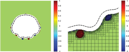34) ) using the variable mesh approach are shown in Figures 3–4. In these figures, the values of the currents obtained are represented by different colours. Note that the values obtained for the dimensionless current densities ${\alpha }_p$ tend to be 0, $+1$ or $-1$, avoiding intermediate values. Note that the equilibrium shapes for the optimized configuration of electric currents were obtained and represented in the figures together with the target shapes. The figures show that in these examples the equilibrium shapes fit very well the target shapes considered.

Figure 2. First and second examples. The thick black lines represent a cut of the equilibrium liquid metal surface by a meridian plane. Plus signs: location in the meridian plane of positive currents, i.e. flowing in the direction opposite to the reader. Minus signs: negative currents. Numbers in parentheses give the inductor coordinates.

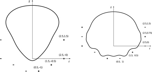
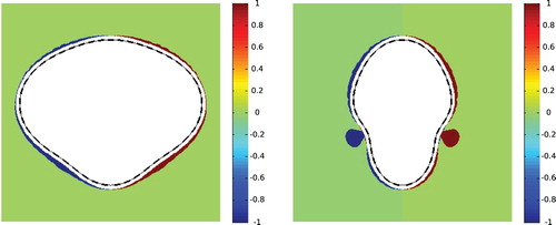
Figure 3. Left: solution of the first example for $\rho =1\times {10}^{-7}$, right: detail of the solution. Dashed line: target shape, thin solid line: equilibrium shape obtained for the optimized electric currents. The colours of the cells indicate the value ${\alpha }_p$ of the current density according to the scale of the colour bar.

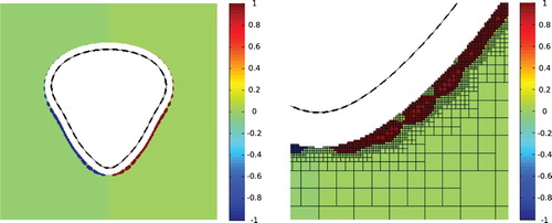
Figure 4. Left: solution of the second example for $\rho =1\times {10}^{-7}$, right: detail of the solution. Dashed line: target shape, thin solid line: equilibrium shape obtained for the optimized electric currents. The colours of the cells indicate the value ${\alpha }_p$ of the current density according to the scale of the colour bar.

The third and fourth examples correspond to shapes Γ given by the expression$r=R\left(\eta \right)\sin \left(\eta \right)$, $z=R\left(\eta \right)\cos \left(\eta \right)$ with $\begin{array}{rl}R\left(\eta \right)& =1+{\epsilon }_1\left[P_0\right(\cos \left(\eta \right))-P_2(\cos \left(\eta \right)\left)\right]+{\epsilon }_2\left[P_0\right(\cos \left(\eta \right))-P_4(\cos \left(\eta \right)\left)\right]\\ & +{\epsilon }_3\left[P_1\right(\cos \left(\eta \right))-P_3(\cos \left(\eta \right)\left)\right],\end{array}$ where $P_{\ell }$ is the ℓ-degree Legendre polynomial. For this representation the value ${\epsilon }_3=0.1$ ensures an equal value for $\mathcal{C}+z$ at the poles of the axisymmetric shape. In the third example ${\epsilon }_1=0.2$, ${\epsilon }_3=-0.1$, and in the fourth one ${\epsilon }_1=-0.2$, ${\epsilon }_3=-0.1$. These values ensure that the quantity $\mathcal{C}+z$ be maximal at the poles. The results obtained are shown in Figure 5.

Figure 5. Solution of the third and fourth examples for $\rho =1\times {10}^{-7}$. Dashed line: target shape, thin solid line: equilibrium shape obtained for the optimized electric currents. The colours of the cells indicate the value ${\alpha }_p$ of the current density according to the scale of the colour bar.

The fifth and sixth examples are a sphere and a rounded cylinder. Both examples are not shapable, since the necessary condition of Equation (23(23) $\mathcal{C}\left(y_1\right)+z\left(y_1\right)=\mathcal{C}\left(y_2\right)+z\left(y_2\right)\ge \mathcal{C}\left(y\right)+z\left(y\right)\mathrm{\forall }y\in \mathrm{\Gamma }.$(23) ) is not satisfied. In the case of the sphere, the solution obtained is shown in Figure 6 whilst the solution for the cylinder is shown in Figure 7. Note in these figures that the equilibrium shape around the south pole has a mean curvature clearly greater than that of the target shape. This fact is a consequence of the non-satisfaction of Equation (23(23) $\mathcal{C}\left(y_1\right)+z\left(y_1\right)=\mathcal{C}\left(y_2\right)+z\left(y_2\right)\ge \mathcal{C}\left(y\right)+z\left(y\right)\mathrm{\forall }y\in \mathrm{\Gamma }.$(23) ). Three-dimensional representations of the solutions obtained for the fifth and sixth examples are given in Figure 8.

Figure 6. Left: solution of the fifth example for $\rho =1\times {10}^{-3}$, right: detail of the solution. Dashed line: target shape, thin solid line: equilibrium shape obtained for the optimized electric currents. The colours of the cells indicate the value ${\alpha }_p$ of the current density according to the scale of the colour bar.

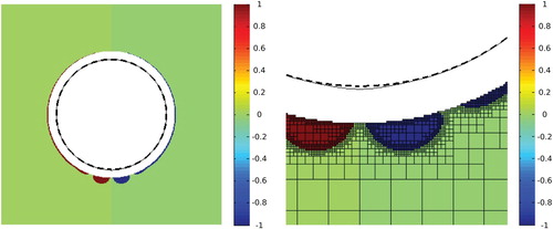
Figure 7. Left: solution of the sixth example for $\rho =1\times {10}^{-3}$, right: detail of the solution. Dashed line: target shape, thin solid line: equilibrium shape obtained for the optimized electric currents. The colours of the cells indicate the value ${\alpha }_p$ of the current density according to the scale of the colour bar.

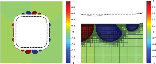
Figure 8. Fifth and sixth examples, a 3D representation of the solutions. Light colour: liquid metal in equilibrium, dark colour: inductors.

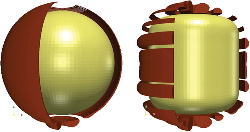
Table 1 presents information about the examples and the results obtained. It can be seen that the optimization algorithm requires less than 30 iterations and a few minutes to solve each of the examples considered.

Table 1. Summary of results.

Example	μ	Cells^a	Iter^a	Time^b (s)	$\mathcal{J}(\varphi -\phi {)}^{\mathrm{c}}$	$\psi (J_{\theta }{)}^{\mathrm{c}}$	ρ^c
Figure 3	20.0	3694	23	164.4	$4.05\times {10}^{-8}$	3.193	${10}^{-7}$
Figure 4	60.0	3258	28	590.7	$1.74\times {10}^{-7}$	1.732	${10}^{-7}$
Figure 5, left	30.0	3958	24	126.2	$2.23\times {10}^{-10}$	0.547	${10}^{-7}$
Figure 5, right	30.0	3675	23	126.7	$5.69\times {10}^{-7}$	0.556	${10}^{-7}$
Figure 6	50.0	3316	22	47.0	$9.75\times {10}^{-6}$	0.339	${10}^{-3}$
Figure 7	50.0	5277	26	129.7	$1.88\times {10}^{-4}$	0.827	${10}^{-3}$

^aNumber of cells and iterations for the final mesh.

^bWall time of the whole process of solution.

^cThe objective function is $\mathcal{J}(\varphi -\phi )+\rho \psi \left(J_{\theta }\right)$.

5. Final remarks

In this paper, we have proposed a new method for solving an inverse problem concerning the design of inductors for three-dimensional EMC applications which is based on topology optimization techniques. A penalization approach is used to obtain stable regular 0-1 solutions for the required configuration of electric currents. The total electric current was considered as the penalty function. It has the advantage of leading naturally to regular 0–1 solutions without introducing a severe smoothing effect or modifying the convex quadratic programming structure of the problem.

The results obtained for the six numerical examples considered show that the method proposed is able to obtain regular 0-solutions with a low total electric current. Since the solutions obtained imply low energy consumption, the method proposed is appropriate from the economic point of view.

From the computational point of view, the method proposed is very attractive, since the optimization problems can be solved very efficiently by using interior-point optimization algorithms. In addition, a simple variable mesh approach has been used to obtain a significant reduction in the number of unknowns, enabling us to obtain solutions with a good resolution at a reasonable computational cost.

Disclosure statement

No potential conflict of interest was reported by the authors.

Additional information

Funding

The authors thank the Brazilian research councils CAPES, CNPq and FAPERJ, the institutions supporting the programme Ciência Sem Fronteiras of Brazil, the Uruguayan research councils ANII and CSIC, and the French research council CNRS for the financial support.

Notes

1 We use here the usual definition in fluid mechanics, i.e. $\mathcal{C}={\kappa }_1+{\kappa }_2$, where ${\kappa }_1$ and ${\kappa }_2$ are the principal curvatures of the surface, e.g. a sphere of liquid metal of radius r has positive curvatures ${\kappa }_i=1/r$, providing $\mathcal{C}=2/r$.

References

- Zhiqiang C, Fei J, Xingguo Z, et al. Microstructures and mechanical characteristics of electromagnetic casting and direct-chill casting 2024 aluminum alloys. Mater Sci Eng A. 2002;327:133–137. doi: 10.1016/S0921-5093(01)01673-2
- Fu HZ, Shen J, Liu L, et al. Electromagnetic shaping and solidification control of Ni-base superalloys under vacuum. J Mater Process Technol. 2004;148:25–29. doi: 10.1016/j.jmatprotec.2003.11.039
- Besson O, Bourgeois J, Chevalier PA, et al. Numerical modelling of electromagnetic casting processes. J Comput Phys. 1991;92:482–507. doi: 10.1016/0021-9991(91)90219-B
- Shercliff JA. Magnetic shaping of molten metal columns. Proc R Soc Lond A. 1981;375:455–473. doi: 10.1098/rspa.1981.0063
- Mestel AJ. Magnetic levitation of liquid metals. J Fluid Mech. 1982;117:27–43. doi: 10.1017/S0022112082001505
- Sneyd AD. Fluid flow induced by a rapidly alternating or rotating magnetic field. J Fluid Mech. 1979;92:35–51. doi: 10.1017/S0022112079000513
- Sneyd AD, Moffatt HK. Fluid dynamical aspects of the levitation-melting process. J Fluid Mech. 1982;117:45–70. doi: 10.1017/S0022112082001517
- Li BQ. The magnetothermal phenomena in electromagnetic levitation processes. Int J Eng Sci. 1993;31:201–220. doi: 10.1016/0020-7225(93)90034-R
- Moffatt HK. Magnetostatic equilibria and analogous Euler flows of arbitrarily complex topology. Part 1. Fundamentals. J Fluid Mech. 1985;159:359–378. doi: 10.1017/S0022112085003251
- Bui RT. Computational modelling of thermophysical processes in the light metals industry. Rev Gén Therm. 1997;36:575–591. doi: 10.1016/S0035-3159(97)89985-0
- Dulikravich GS, Lynn SR. Unified electro-magneto-fluid dynamics (EMFD): introductory concepts. Int J Non-Linear Mech. 1997;32:913–922. doi: 10.1016/S0020-7462(96)00084-4
- Dulikravich GS, Lynn SR. Unified electro-magneto-fluid dynamics (EMFD): a survey of mathematical models. Int J Non-Linear Mech. 1997;32:923–932. doi: 10.1016/S0020-7462(96)00083-2
- Dennis BH, Dulikravich GS. Magnetic field suppression of melt flow in crystal growth. Int J Heat Fluid Flow. 2002;23:269–277. doi: 10.1016/S0142-727X(02)00174-1
- Dulikravich GS, Colaço MJ. Convective heat transfer control using magnetic and electric fields. J Enhanc Heat Transf. 2006;13:139–155. doi: 10.1615/JEnhHeatTransf.v13.i2.40
- Colaço MJ, Dulikravich GS. A multilevel hybrid optimization of magnetohydrodynamic problems in double-diffusive fluid flow. J Phys Chem Solids. 2006;67:1965–1972. doi: 10.1016/j.jpcs.2006.05.036
- Bay F, Labbe V, Favennec Y, et al. A numerical model for induction heating processes coupling electromagnetism and thermomechanics. Int J Numer Methods Eng. 2003;58:839–867. doi: 10.1002/nme.796
- Coulaud O, Henrot A. Numerical approximation of a free boundary problem arising in electromagnetic shaping. SIAM J Numer Anal. 1994;31:1109–1127. doi: 10.1137/0731058
- Coulaud O. Multiple time scales and perturbation methods for high frequency electromagnetic-hydrodynamic coupling in the treatment of liquid metals. Nonlinear Anal-Theor. 1997;30:3637–3643. Proceedings of the Second World Congress of Nonlinear Analysts. doi: 10.1016/S0362-546X(97)00264-2
- Coulaud O. Asymptotic analysis of magnetic induction with high frequency for solid conductors. RAIRO Modél Math Anal Numér. 1998;32:651–669. doi: 10.1051/m2an/1998320606511
- Brancher JP, Etay J, Séro-Guillaume O. Formage d'une lame métallique liquide. Calculs et expériences. J Méc théor appl. 1983;2:977–989.
- Brancher JP, Séro-Guillaume OE. Étude de la déformation d'un liquide magnétique. Arch Ration Mech Anal. 1985;90:57–85. doi: 10.1007/BF00281587
- Henrot A, Brancher JP, Pierre M. Existence of equilibria in electromagnetic casting. In: Proceedings of the Fifth International Symposium on Numerical Methods in Engineering, Vol. 1, 2 (Lausanne, 1989). Comput. Mech., Southampton; 1989. p. 221–228.
- Henrot A, Pierre M. Un problème inverse en formage des métaux liquides. RAIRO Modél Math Anal Numér. 1989;23:155–177. doi: 10.1051/m2an/1989230101551
- Felici TP, Brancher JP. The inverse shaping problem. Eur J Mech B Fluids. 1991;10:501–512.
- Felici TP. The inverse problem in the theory of electromagnetic shaping. University of Cambridge; 1992.
- Pierre M, Roche JR. Computation of free surfaces in the electromagnetic shaping of liquid metals by optimization algorithms. Eur J Mech B Fluids. 1991;10:489–500.
- Pierre M, Roche JR. Numerical simulation of tridimensional electromagnetic shaping of liquid metals. Numer Math. 1993;65:203–217. doi: 10.1007/BF01385748
- Pierre M, Rouy E. A tridimensional inverse shaping problem. Commun Part Diff Eq. 1996;21:1279–1305. doi: 10.1080/03605309608821226
- Shin J, Spicer JP, Abell JA. Inverse and direct magnetic shaping problems. Struct Multidiscip Optim. 2012;46:285–301. doi: 10.1007/s00158-011-0756-2
- Canelas A, Roche JR, Herskovits J. The inverse electromagnetic shaping problem. Struct Multidiscip Optim. 2009;38:389–403. doi: 10.1007/s00158-008-0285-9
- Canelas A, Roche JR, Herskovits J. Inductor shape optimization for electromagnetic casting. Struct Multidiscip Optim. 2009;39:589–606. doi: 10.1007/s00158-009-0386-0
- Roche JR, Canelas A, Herskovits J. Shape optimization for inverse electromagnetic casting problems. Inverse Probl Sci Eng. 2012;20:951–972. doi: 10.1080/17415977.2011.637206
- Canelas A, Novotny AA, Roche JR. A new method for inverse electromagnetic casting problems based on the topological derivative. J Comput Phys. 2011;230:3570–3588. doi: 10.1016/j.jcp.2011.01.049
- Canelas A, Roche JR. Topology optimization in electromagnetic casting via quadratic programming. Inverse Probl Sci Eng. 2014;22:419–435. doi: 10.1080/17415977.2013.788173
- Felici TP. On the surface stability of liquid conductors in electromagnetic shaping. J Fluid Mech. 1995;302:1–28. doi: 10.1017/S0022112095003983
- Canelas A, Herskovits J, Telles JCF. Shape optimization using the boundary element method and a SAND interior point algorithm for constrained optimization. Comput Struct. 2008;86:1517–1526. doi: 10.1016/j.compstruc.2007.05.008
- Kohn R, Vogelius M. Determining conductivity by boundary measurements. Commun Pure Appl Math. 1984;37:289–298. doi: 10.1002/cpa.3160370302
- Jackson JD. Classical electrodynamics. New York (NY): Third Wiley; 1998.
- Gagnoud A, Etay J, Garnier M. Le problème de frontière libre en lévitation électromagnétique. J Méc Théor Appl. 1986;5:911–934.
- Novruzi A, Roche JR. Second order derivatives, Newton method, application to shape optimization. Rapport de recherche RR-2555, INRIA; 1995.
- Roche JR. Gradient of the discretized energy method and discretized continuous gradient in electromagnetic shaping simulation. Appl Math Comput Sci. 1997;7:545–565.
- Roche JR. Adaptive Newton-like method for shape optimization. Control Cybern. 2005;34:363–377.
- Novruzi A, Roche JR. Newton's method in shape optimisation: a three-dimensional case. BIT. 2000;40:102–120. doi: 10.1023/A:1022370419231
- Atkinson KE. The numerical solution of integral equations of the second kind. Cambridge: Cambridge University Press; 1997. (Cambridge Monographs on Applied and Computational Mathematics; 4).
- Becker AA. The boundary element method in engineering: a complete course. New York (NY): McGraw-Hill; 1992.
- Sullivan CR. Optimal choice for number of strands in a litz-wire transformer winding. IEEE Trans Power Electron. 1999;14:283–291. doi: 10.1109/63.750181
- Brebbia CA, Telles JCF, Wrobel LC. Boundary element technique: theory and applications in engineering. Berlin: Springer-Verlag; 1984.