A combined neural network and simulated annealing based inverse technique to optimize the heat source control parameters in heat treatment furnaces

Abstract

This study proposes the use of artificial neural network (ANN) based surrogate framework along with simulated annealing (SA) approach to inversely estimate the optimum values of heat source control parameters in a heat treatment furnace. In particular, a two-dimensional radiant furnace with gas fired heaters has been considered and the heat source control parameters for a general gaussian heating profile are estimated to achieve better heat flux uniformity at the specimen. To expedite the forward radiative transfer calculations, ANN based surrogate is developed and coupled with SA. The maximum difference in radiative transfer solution and ANN is found to be less than 6%. Results indicate that the uniformity of fluxes is largely dependent on the emissivity of the specimen and its overall length, the dependence on specimen temperature and gas concentration is minimal. Cross validation of optimum heating profiles with radiative transfer solver shows an excellent match in local heat flux predictions. Overall, combined ANN-SA based algorithm proves to be an accurate and fast tool in heat source control parameter optimization problem.

Keywords:

• Inverse solution
• heat source
• ANN
• optimization

2010 Mathematics Subject Classifications:

• 80A23
• 65K10

1. Introduction

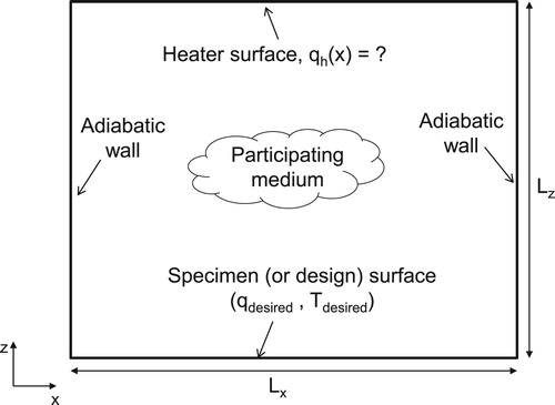
Application of common heat treatment furnaces can be found in material processing, concentrated solar power systems, thermal processing of semi-conductor wafers, baking of food items, curing of paints and dyes etc. The heat treatment furnaces, in general, have a heater surface (usually at the top) where the discrete heaters or burners are mounted and a specimen surface (usually at the bottom) that hosts the specimen to be heat treated. At the heater surface, gas fired burners or electric heaters are mounted and the primary job of these heaters is to heat the specimens to a desired level of temperature in order to impart uniform material properties. Since the operating temperatures are quite high, radiation appears to be a dominant mode of heat transfer. For instance, in applications such as cake baking and aluminum reheating, radiation itself accounted for 75–80% of the total heat transfer to the specimen [1,2]. In case the heating operation is performed through gas fired heaters, there are also participating gases present in the furnace which play a significant role in radiation heat transfer [3,4]. Modeling and prediction of radiative heating from the gas fired heaters to the specimen in the presence of participating medium is important to evaluate the performance of the furnace and efficiency of heating. This is accomplished either by measurements or by numerical modelling of radiative transfer phenomenon i.e. by solving the complete radiative transfer equation (RTE). The basic goal of the heat treatment is to provide uniform heating to the specimens, and the task before a furnace operator is to adjust the different operation parameters such as placements of the heaters and heater power levels to achieve this. From the modelling point of view, this task requires to specify two boundary conditions on the specimen surface namely the desired temperature and the desired heat flux, whereas no boundary condition is known at the heater surface (see Figure 1). This problem belongs to the class of inverse thermal design [5]. The traditional way to tackle this is to use the trial and error method, where based on the experience of the furnace operator, the heating conditions are tuned sequentially until the desired effect is obtained at the specimen. It is both time consuming and unscientific. With the rise of computing era and simultaneous mathematical development of inverse problems for radiation, the problem has more scientifically approachable solutions. Within the framework of inverse modelling, the major problem arises due to non-linear nature of the radiative transfer equation. This results in the ill-conditioned matrices, the solution to which may give unphysical results. Several researchers in the past have attempted to solve this problem by using regularization techniques [5,6]. The idea behind regularization methods is to reduce the ill-posed nature of the problem by using sophisticated techniques, some of them include singular value decomposition, modified singular value decomposition and Tikonov regularization [7]. An elaborate review and comparison of various regularization methods can be found elsewhere [8,9].

Figure 1. A typical inverse problem of determining unknown heater conditions in a heat treatment furnace.

The other possible way is to treat the problem as an optimization problem, such that the objective function is formulated in a way that the error between the obtained and desired effect should be minimum. Therefore, the output of optimization algorithm is the best design which ensures that the desired goal is achieved. In particular to the furnaces with discrete heaters, two design problems appear to be really important, (i) optimum number and placement of the heaters and (ii) the optimum distribution of the power across the heaters. During the heat treatment process, the heat from the heaters is dissipated to the participating medium, which in turn heats the specimen. Knowing the desired heat flux required at the specimen, one can calculate the total heat needed to be supplied to the heaters, however, the uniformity of the heat flux at the specimen surface largely depends upon the heater configuration and distribution of power. Controlling these two factors can ensure better uniformity in heating and hence increased efficiency of the process. Considering the discrete nature of the problem, researchers have directed their attention towards applying search based optimization algorithms to obtain the optimum heater conditions. To obtain the solution of the aforementioned two class of inverse design problems with different geometries and boundary conditions, the optimization methods that have been primarily applied include generalized extreme optimization [10,11], hybrid-genetic algorithm [12,13], micro-genetic algorithm [14–16], particle swarm optimization [17] and krill herd optimization [18]. Overall, optimization methods have proved to be sufficiently accurate in obtaining the results in such inverse problems. However, in all the problems discussed and solved so far, the primary attention has been laid on using new and efficient optimization algorithms in solving these problems. A little attention has been directed towards the fact that the actual forward estimation (i.e. by solving the full radiative transfer model) tend to consume enormous computation time, due to which overall process becomes very slow. This can be overcome by developing efficient surrogate models from the accurate forward model data. Some of the standard methods to develop a surrogate model include high order singular value decomposition, polynomial based regression, radial basis functions method and neural networks. A review and application of some of these methods is included in [19]. Among these, neural networks have appeared to be a promising choice due to their applicability to a variety of complex non-linear problems. In particular to radiative transfer problems, Howell et al. [20] used a neural network model to provide efficient control over transient heating systems. Yeun et al. [21] developed ANN based emissivity functions to calculate radiative transfer in gray and non-gray media. The applicability of these functions was also analysed in combustion mixtures by the same authors [22]. It is observed that use of neural network as a surrogate model to some of the standard radiative transfer problem have been made in the past, efforts towards assessing its capability as a possible alternate tool to predict the radiative heating in inverse problems are rare.

Recently, author has proposed the use of a neural-network based surrogate model and utilized it to obtain the optimum number and placement of discrete heaters in a radiant furnace [23]. To perform the optimization, surrogate model was coupled with a genetic algorithm. It was seen that this method was able to efficiently obtain the solution to discrete heater number and placement optimization problem. This addressed the applicability of neural network modelling to the first type of inverse problems as discussed before. However, there remains to investigate the second type of problem, where, to obtain the desired conditions on the specimens, it is required to optimize the input heat flux distribution to the heaters. Therefore, this study addresses the problem of optimizing the heat source control parameters for obtaining a desired level of uniform heating at the specimen surface using a neural network based surrogate modelling and coupling it with simulated annealing. The heat treatment furnace is approximated as a two dimensional rectangular geometry and is equipped with discrete heaters at the top surface. The number of heaters is fixed while the power input to the heaters is approximated by a general Gaussian profile with defined maximum and minimum power levels. The bottom wall is considered as the specimen surface and the heat fluxes are monitored at five discrete locations of the specimen surface. In order to impart uniform heating to the specimen surface, the parameters of the Gaussian profile can be varied. The problem then breaks down to optimize the control parameters such that the specimen surface receives a uniform heating of desired level at desired temperature. Firstly, a neural network based surrogate is developed from the data generated by the forward RTE solver. This network is then coupled with Simulated Annealing algorithm to solve the multi-variable optimization problem to obtain optimum values of heat source control parameters. The following sections represent the mathematical formulation, development procedure and inverse solution using ANN-SA algorithm.

2. Formulation of the problem

2.1. The forward model: solution to radiative transfer equation

To determine the heat fluxes received at the specimen surface, a forward model is developed following the Finite Volume Method (FVM) [24] as the solver for radiative transfer equation and Spectral Line based Weighted sum of gray gases (SLW) method [25] for incorporation of non gray nature of participating medium. The detailed description of the governing equations and development procedure is throughly discussed in references [23, 26]. Only the important equations are provided here. For a two dimensional rectangular geometry, the change in radiation intensity in a particular direction as it passes through a control volume dV characterized by the dimensions dx and dz and hosts the participating medium with ${\kappa }_{g,\lambda }$ as the spectral absorption coefficient, is given as (1) $\mu \frac{\mathrm{\partial }{I}_{\lambda }^{\prime }}{\mathrm{\partial }x}+\eta \frac{\mathrm{\partial }{I}_{\lambda }^{\prime }}{\mathrm{\partial }z}=-{\kappa }_{g,\lambda }{I}_{\lambda }^{\prime }+{\kappa }_{\lambda }{I}_{b\lambda }$(1) Where μ and η respectively denote the direction cosines in the x and z directions. The left hand side of above equation represent the change in directional spectral radiation intensity with respect to position while the right hand side denotes the attenuation and augmentation because of medium absorption and emission of the radiation intensity respectively. As can be observed, Equation (1(1) $\mu \frac{\mathrm{\partial }{I}_{\lambda }^{\prime }}{\mathrm{\partial }x}+\eta \frac{\mathrm{\partial }{I}_{\lambda }^{\prime }}{\mathrm{\partial }z}=-{\kappa }_{g,\lambda }{I}_{\lambda }^{\prime }+{\kappa }_{\lambda }{I}_{b\lambda }$(1) ) is a first order differential equation and one boundary condition should be defined for its solution. This is provided from the intensity balance at the diffuse gray wall, as (2) $I_{\lambda }^{\prime }(r)={ϵ}_w{I}_{bw}+\frac{1-{ϵ}_w}{\pi }{\int }_{n_w\mathrm{\Omega }<0}{I}_{\lambda }|n_w.\mathrm{\Omega }|\mathrm{d}\mathrm{\Omega }$(2) Where the term on the left side indicates the outgoing intensity at the wall location r, and the terms on the right hand side indicate the contribution of hemispherical emission and reflection to the outgoing intensity. Equation (1(1) $\mu \frac{\mathrm{\partial }{I}_{\lambda }^{\prime }}{\mathrm{\partial }x}+\eta \frac{\mathrm{\partial }{I}_{\lambda }^{\prime }}{\mathrm{\partial }z}=-{\kappa }_{g,\lambda }{I}_{\lambda }^{\prime }+{\kappa }_{\lambda }{I}_{b\lambda }$(1) ) along with boundary condition as defined by Equation (2(2) $I_{\lambda }^{\prime }(r)={ϵ}_w{I}_{bw}+\frac{1-{ϵ}_w}{\pi }{\int }_{n_w\mathrm{\Omega }<0}{I}_{\lambda }|n_w.\mathrm{\Omega }|\mathrm{d}\mathrm{\Omega }$(2) ) can be solved numerically using Finite Volume Method (FVM) both in spatial as well as angular domain. The detailed discretization based on FVM has been provided in the literature and the development methodology is prescribed in [23]. There remains a need to define the spectral absorption coefficient for a mixture of gases in a control volume. This is obtainable through the SLW method, inherently developed on the concepts of absorption line blackbody distribution function [27] and later extended to include mixture of gases [28]. Within the framework of SLW model, sometimes it is customary to define the total emissivity representative of the mixture of participating gases, which is given as: (3) $ϵ=\sum _{j=0}^{NGG}{u}_j(T)(1-{\mathrm{e}}^{-{\kappa }_{j}L})$(3) where NGG is the total number of gray gases considered in the SLW model and ${\kappa }_j$ is the representative absorption coefficient for the $j\mathrm{th}$ gray gas. L denotes the average path length or mean beam length, which can be defined based on the control volume under inspection or based on the volume of the whole enclosure. However, the RTE usually requires the absorption coefficient value for the given volume which can be calculated as: (4) $\kappa =-\frac{1}{L}\ln (1-ϵ)$(4) With the κ obtained from Equation (4(4) $\kappa =-\frac{1}{L}\ln (1-ϵ)$(4) ), the problem can be solved assuming the medium to be gray. Although being a gray model, it is usually more reliable than other gray approximations as spectral line contributions are taken into account through individual gray gas coefficients. Amiri et al. [29] has shown that this SLW gray model performs significantly better than Planck's gray model and provides results with acceptable accuracy. Such a model is promising in cases such as radiative equilibrium, where the intensity computation is coupled with temperature distribution of the medium and an iterative procedure is required. An in-house code developed following the FVM and SLW method has been verified with the benchmark results and is chosen as the forward model for the present study.

2.2. The surrogate model: artificial neural networks

Artificial neural networks are one of the promising way to develop a surrogate model possibly for a variety of problems. The fundamentals of neural networks finds its root in the functioning of a natural neuron, which works as an information processing tool. A single neuron takes certain information as input and processes it to achieve some specific output. A neural network is a group of such neurons. An artificial neural network, therefore, is a group of neurons, which uses certain mathematical functions to obtain the output from the given set of input. These mathematical functions are called transfer (or mapping) functions. Specifically, a neural network performs the mapping of a set of inputs $M::\{x_1,x_2,x_3,\dots ,x_m\}$ to a set of outputs $O::\{O_1,O_2,O_3,\dots ,O_n\}$ following a transfer function $f(x)$. 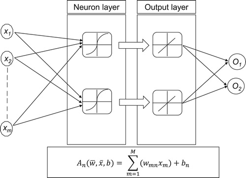Some of the most commonly used transfer functions are tangent-sigmoid, logistic-sigmoid, rectified linear unit, pure linear transfer function etc. The connections between input-output dataset, neurons and the flow of information between them decides the network architecture. A typical neural network, most commonly used in engineering application is a feed-forward back propagation network as shown in Figure 2. It has distinct layer of inputs and outputs and the neurons. The information from the input layer is feed to the neuron layers, which perform the mapping and further send the information to subsequent neuron layers. In case there are no other neuron layers, the output layer, in general performs a linear mapping of the information, such that $f(A)=A$. Each input connection to a neuron is characterized by a weight ($w_{mn}$), which is nothing but the contribution of an input towards the transfer operation to be performed by the neuron. There is also a parameter called bias ($b_n$) associated with every neuron in the layer. Together, the weight and bias quantify the contribution from each input and their sum over all the inputs forms the argument ($A_n$) for the transfer operation. Any standard transfer function ($T(A_n)$) is then utilized to generate the output from the neuron arguments. Considering that a static dataset of input-output values is available, the neural network initially assigns assumed values to weights and bias and calculates the output. The obtained outputs are matched with the actual output and based on the values of the errors, the weights and bias are readjusted. This is repeated for all the available datasets until the overall error is minimum. In this way the network gets trained for a set of input variables for their specified range. This is called training of the network and the popular methods to perform training include Levenberg-Marquardt [30], Scaled Conjugate Gradient [31] and Bayesian Regularization [32]. Within the network training algorithm, there is provision to divide the complete dataset into dataset for training and testing. Upon having sufficient confidence on the network performance over these two class of data, the network should further be validated with a completely new dataset which was neither a part of training nor testing.

Figure 2. A typical feed-forward back propagation neural network framework.

3. The test problem of heat treatment furnace

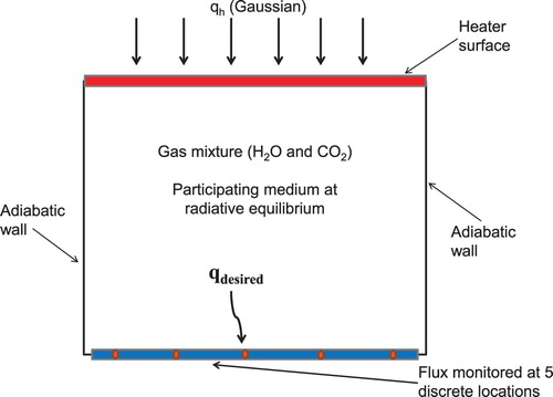
The test problem considered in the present study is a heat treatment furnace approximated as a two-dimensional rectangular geometry with the upper surface hosting the heaters and the bottom surface hosting the specimens, as shown in the Figure 3. The heaters size and shape are uniform and they occupy the complete heater surface. The furnace contains a mixture of participating gases viz. ${\mathrm{H}}_2\mathrm{O}$ and ${\mathrm{CO}}_2$ in varied proportions. The side walls are adiabatic. As the process of heating starts, the heaters dissipate heat into the medium, thereby changing the thermal conditions of the medium. However, over the time, the medium adjusts itself to allow all the heat to pass through it and eventually comes to a steady state. This is called radiative equilibrium. The properties of the medium have a strong effect on time taken to achieve the equilibrium. This is one of the main reason that the forward RTE model becomes slow in some of the cases where the media is in optically thin limit. The RTE based forward model estimates the net radiative heat fluxes at the specimen surface, and major inputs to the given problem are specimen temperature ($T_{des}$), specimen emissivity (${ϵ}_d$), gas concentration ($Y_{\mathrm{H}2\mathrm{O}}$) and heat input to the heaters ($q_h$). The concentration of ${\mathrm{CO}}_2$ gas is assumed to be half of ${\mathrm{H}}_2\mathrm{O}$ gas concentration for all cases (i.e. $Y_{\mathrm{CO}2}=Y_{\mathrm{H}2\mathrm{O}}/2$), which is standard for many of the combustion applications. The design requirement, as mentioned earlier, is the uniform desired heat flux on the specimen surface to maintain the specimen temperature at steady state. To achieve this, the input heat flux variation at the heater surface ($q_h(x)$) can be controlled. We assume a general Gaussian profile of the form, (5) $q_h(x)=a{\mathrm{e}}^{-(x-b{)}^2/2c^2}$(5) Where, the term a, b and c are the control parameters of the profile. In physical sense, the value of a signifies the peak value of heat flux, b determines the location of the peak and c indicates the extent or spread of the profile over the heater surface length. A high value of c indicates a broader spread or gradual change in the heat flux values from one location to the other, while a value of c close to 0 signifies a narrow spread or sharp change. It is customary to note that a has the units of heat flux i.e. 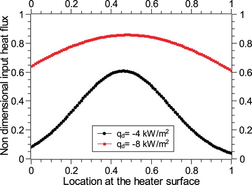${\mathrm{W}/\mathrm{m}}^2$ and therefore on non-dimensionalizing a, non-dimensional heat flux profile can be generated. In this case, a value of a close to 1 would signify that peak flux value in profile is close to the maximum possible flux input and a value of a close to 0 would signify that peak flux value in profile is close to the minimum possible flux input. This type of representation of heat flux profile is very practical [33] and allows one to examine variety of profiles for a given problem and therefore ensures better control. Considering all other inputs to the problem are defined, the question before us is to obtain the best values of a, b and c which can fulfill the requirements of desired and close to uniform heat fluxes at the specimen surface.

Figure 3. Depiction of a heat treatment furnace with heater and specimen surface.

4. Validation of the accuracy of forward model

4.1. Validation for a two dimensional rectangular geometry

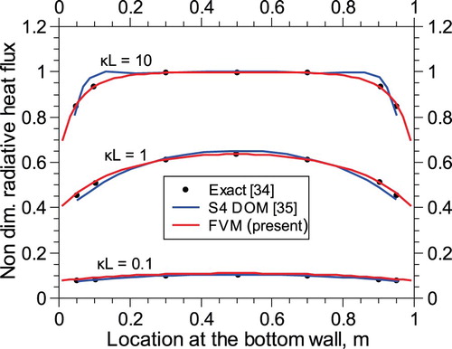
A two-dimensional rectangular furnace with a medium that can absorb and emit, but does not scatter has been considered for the purpose of validation of the present methodology. This case belongs to the benchmark solutions discussed by Lockwood et al. [34], who developed an exact solution for this problem. This was further solved by Jamaluddin et al. [35] using the discrete ordinates method. The enclosure has cold and black walls and medium with varying optical depth from $\kappa L=0.1$, 1 and 10. The radiative heat flux to the bottom wall has been estimated for these optical depths and the results are shown in Figure 4. From the figure, it can be observed that the present FVM-SLW Gray formulation gives better accuracy than the S4-Discrete Ordinates Method (DOM) where S4 indicates that 24 discrete directions are used in DOM. The maximum errors observed in the flux estimation are less than 8% for the optically thin case and less than 1% for optically thick case.

Figure 4. Validation of present FVM formulation for a two dimensional rectangular enclosure with homogeneous and gray participating medium – comparison of solutions with exact method and S4 DOM.

4.2. Verification with a commercial solver

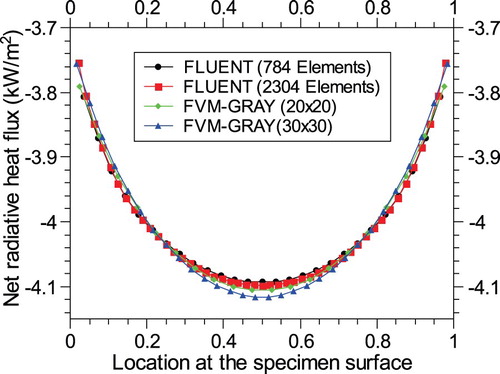
Additional to the above mentioned case, the forward model based on the FVM-SLW framework to solve the radiative transfer equation (Section 2.1) has been thoroughly verified against the existing benchmark cases in the literature and the detailed discussion on the same has been presented in the reference [23]. However, a more relevant verification of the formulation and code has also been performed with respect to solutions from ANSYS-FLUENT [36]. For the purpose of verification with the case of heat flux boundary conditions pertinent to this case, solutions are generated using the Discrete Ordinates module. The enclosure is $1\mathrm{m}\times 1\mathrm{m}$ with homogeneous participating medium inside. Temperature and emissivity of the specimen surface is 400 K and 0.4 respectively. The case under consideration has been modelled with constant horizontal heating profile at the top wall ($Q_h=4000\mathrm{W}$) and the values of net radiative heat flux across the specimen surface is evaluated. The side walls are all adiabatic. The distribution of the heat fluxes at the bottom wall is plotted with respect to the wall location and is represented in Figure 5. It can be clearly observed from the figure that the present forward model agrees well with the results obtained through ANYSYS-FLUENT for both coarse and fine meshes. The change in values of the fluxes on refining the grid from $20\times 20$ to $30\times 30$ did not produce a significant change. In a similar way, the angular grids are also refined from a value $6\times 4$ to $8\times 6$. The relative errors in the estimation of mean heat fluxes at the specimen surface upon doing the spatial and angular grid refinement are found to be less than 0.1% in both cases. Based on these results, the grid sizes in spatial domain is fixed to $20\times 20$ and the grid sizes in angular domain is fixed to $6\times 4$ for the generation of forward model output data for building a neural network to drive the inverse problem.

Figure 5. Verification of the forward RTE model with the results from ANSYS-FLUENT, for a case of heating surface at the top with $Q_h=4000\mathrm{W}$, $T_d=400\mathrm{K}$, ${ϵ}_d=0.4$, $\kappa =1$.

5. Development of ANN as a surrogate model

The heat treatment furnace geometry shown in Figure 3 has been considered for the purpose of development and testing of a neural network based surrogate model and in order to use it to expedite the forward calculations in the inverse problem. The furnace geometry is $1\mathrm{m}\times 1\mathrm{m}$, which contains a gas mixture of participating gases such as ${\mathrm{H}}_2\mathrm{O}$ and ${\mathrm{CO}}_2$. The heat input in the form of a Gaussian curve (Equation (5(5) $q_h(x)=a{\mathrm{e}}^{-(x-b{)}^2/2c^2}$(5) )) has been supplied to the heaters and the FVM-SLW based RTE solver calculates the heat fluxes at the specimen surface. The side walls are adiabatic and the total radiative heat flux values are monitored at the specimen surface at five discrete locations (viz $x=0.1,0.3,0.5,0.7$ and 0.9) as shown in Figure 3. For the purpose of developing the network as the surrogate to the RTE solver, a set of 200 cases were generated using Latin Hypercube Sampling (LHS) [37]. The range of input variables has been shown in Table 1. Values of the control parameter a has been defined such that $a_k=q_{h,k}/q_{h,max}$, where $q_{h,k}$ is the value of peak heat flux for the $k\mathrm{th}$ case and $q_{h,max}$ is the maximum allowable heat flux value. In order to obtain the actual flux value from a non-dimensional heat flux, a simple relation is used, which is given as, $q_h=(q_{h,max}-q_{h,min})\ast q_{h,ndm}+q_{h,min}$. Where, $q_{h,max}$ is the maximum possible heat flux value, $q_{h,min}$ is the minimum possible heat flux value and $q_{h,ndm}$ is non-dimensional heat flux value as obtained from Equation (5(5) $q_h(x)=a{\mathrm{e}}^{-(x-b{)}^2/2c^2}$(5) ). The values of maximum and minimum allowable heat fluxes pertinent to present study has been shown in Table 1. The RTE model is run for these 200 sets of input and the outputs are generated. These 200 input-output datasets are now utilized to generate the neural network with the help of Neural Network toolbox in MATLAB [38]. This can be highlighted that 5 out of 6 input variables have their specified range between 0 to 1 (Table 1). The values of a, b, c and emissivity ranges from 0 to 1. The ${\mathrm{H}}_2\mathrm{O}$ gas concentration ranges from 0 to 0.25. The only variable needs to be normalized is specimen temperature which ranges from 300 K to 600 K. The normalization of specimen temperature is made as $T/T_{max}$, where $T_{max}=600\mathrm{K}$. Before introducing to MATLAB, this 200 input-output dataset was divided into two parts, where 90% of it (180 cases) were used in MATLAB for network generation and 10% of it (20 cases) were kept reserved to perform the external validation of the network. The choice of these external validation cases was randomized in order to maintain generality in the values of input variables. Such a division helps to store some part of the data to be introduced to the network later for the assessment of its accuracy. MATLAB uses the provided datasets in the fractions of 70% for training, 15% for testing and 15% for internal validation. We choose Bayesian regularization [32] as the training algorithm as it ensures that there is no overfitting in terms of number of connections and number of variables, and always choses the optimum number of connections to define the network. It also uses all the dataset that is made available to the algorithm. The training has been performed using both single and double neuron layer, however in the present case, the single layer networks did not provide satisfactory results and hence a two layer network was chosen. With a two layer network, assessment of the network performance is judged based on three different performance criteria i.e. training error, testing error and external validation error. Out of these, in order to avoid an overfitting situation, the external validation error has been monitored closely since it corresponds to the data which was totally new to the network. The values of mean square error (MSE) for training, testing and external validation are tabulated in Table 2. From the table, it can be observed that the network corresponding to neurons (8,8) i.e. with architecture 6-8-8-5 performs best in terms of MSE value for training and testing as well as external validation. The training and testing results for this network has been shown in Figure 6. Among the other networks listed in Table 2, a network with architecture 6-4-8-5 though shows an acceptable error, but did not converge in training till the maximum number of epochs were reached and so the results are taken at the last epoch. Another network with architecture 6-8-2-5 has comparable values of validation error and converged within 413 epochs. Therefore, to analyse the networks 6-8-2-5 and 6-8-8-5, a separate test is performed with a newly generated set of 5 cases using LHS, the details of which are given in Table 3. The value of relative errors in local heat flux predictions (i.e. 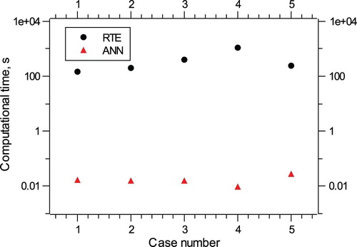$RE=|RTE-ANN|/RTE$) by the network are compared with the actual solution through RTE. The results of this analysis have been included in Table 4 which gives the magnitude of maximum relative error between local heat flux estimation by ANN and the corresponding RTE solution. From the table, it can be observed that the network 6-8-8-5 performs better than 6-8-2-5 in most of the cases, and thus appears to be a better choice for further analysis. This network is selected and the values of relative errors in local heat flux estimations in between the actual RTE output and ANN prediction for aforementioned 5 cases (Table 3) is plotted in Figure 7. It is observed that the ANN based surrogate predicts the heat flux values accurately and the maximum relative error was found to be under 6%. The computational time comparison between the ANN prediction and RTE solution for these 5 cases is performed on an Intel Pentium N3540 2.16 GHz system equipped with 4 GB RAM. The results are plotted in the Figure 8. As can be observed from the figure, the ANN based model is significantly faster than the RTE solver by the order of ${10}^5\mathrm{s}$. This analysis thus provides promising credibility to use ANN as a surrogate model to apply to the present problem under consideration.

Table 1. The input variables and their lower and upper bounds.

Variables	Lower bound	Upper bound	Unit
$T_{des}$	300	600	K
$Q_h$	1000	10000	W
${ϵ}_d$	0	1	–
$Y_{\mathrm{H}2\mathrm{O}}$	0	0.25	–
a	0	1	–
b	0	1	–
c	0	1	–

Table 2. Training, testing and external validation results for a two layer network.

No. of neurons (Layer 1)	No. of neurons (Layer 2)	Training (MSE)	Testing (MSE)	External Validation (MSE)
2	2	0.0010	0.0025	0.0013
2	4	0.0022	0.0068	0.0113
2	6	0.0011	0.0023	0.0012
2	8	6.2216e−04	0.0041	0.0030
4	2	1.2707e−04	1.5607e−04	0.0002
4	4	6.4779e−05	3.1490e−04	0.0001
4	6	2.9405e−05	6.7014e−04	0.0001
4	8	1.3372e−05	3.7479e−04	7.99e−05
6	2	1.3119e−04	4.7743e−04	0.0004
6	4	3.0456e−05	1.2138e−04	0.0001
6	6	1.2226e−05	2.6156e−04	0.0001
6	8	2.2232e−06	9.7349e−04	0.0051
8	2	5.4998e−05	1.6156e−04	9.24e−05
8	4	1.3706e−05	1.2767e−04	0.0001
8	6	3.9394e−06	1.6221e−04	0.0002
8	8	1.8856e−06	1.2503e−04	3.59e−05

Figure 6. Change in training and testing errors with number of epochs for the network 6-8-8-5.

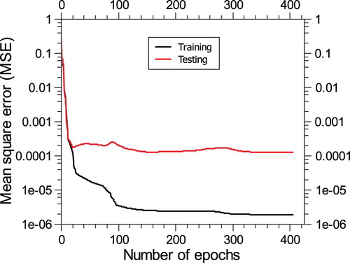
Table 3. Five additional test cases for the validation of the selected network.

case	a	b	c	$T_{des}$	${ϵ}_d$	$Y_{\mathrm{H}2\mathrm{O}}$
1	0.1	0.3	0.3	390	0.9	0.125
2	0.9	0.5	0.5	450	0.7	0.225
3	0.3	0.9	0.7	570	0.3	0.175
4	0.5	0.1	0.9	510	0.1	0.075
5	0.7	0.7	0.1	330	0.5	0.025

Table 4. Magnitude of maximum relative errors in prediction of local heat fluxes for 5 additional test cases as given in Table 3 using two networks with architecture 6-8-2-5 and 6-8-8-5.

Case no.	Maximum relative error (network 6-8-2-5)	Maximum relative error (network 6-8-8-5)
1	0.06247	0.02631
2	0.01276	0.00220
3	0.02020	0.03590
4	0.03096	0.02284
5	0.02101	0.05065

Figure 7. Relative error in flux estimation between ANN and RTE for 5 additional cases generated for validation of the network as given in Table 3.

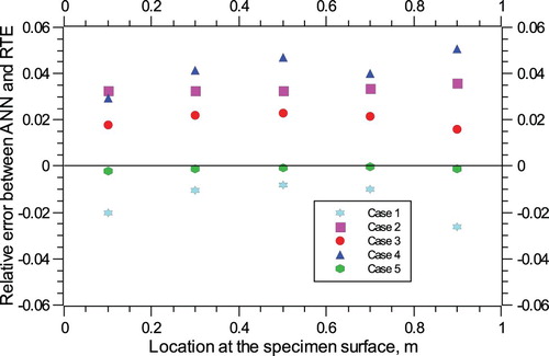
Figure 8. Comparison of computational time in flux estimation between ANN and RTE for 5 additional cases generated for validation of the network as given in Table 3.

6. Setting up the inverse problem

The necessity of determining the optimum heat source control parameters such that to get a desired and close to uniform heat fluxes at the specimen surface is a problem of real practical interest. Here, we consider a similar case, where the specimen surface is imposed with two design conditions and the gaussian flux input at the heater surface should be optimized in such a way that both the design conditions are met. For this purpose we generate two pseudo design cases (see Table 5) where the input parameters such as specimen temperature ($T_{des}$), specimen emissivity (${ϵ}_d$) and ${\mathrm{H}}_2\mathrm{O}$ gas concentration ($Y_{\mathrm{H}2\mathrm{O}}$) have been fixed to a certain assumed value, but are subject to parametric study in the later part. The desired heat flux at the specimen surface is designated as $q_{desired}$ or in short $q_d$. A negative value of desired heat flux means that the net heat fluxes are into the specimen and hence would provide heating. The objective of the problem is to determine the best values of heat flux control parameters a, b and c such that the obtained heat fluxes are nearly uniform and close to the $q_{desired}$ value. Therefore, for a proposed set of control parameters ζ, the objective function is defined as, (6) $F(\zeta )=min(\sum _i(q_{desired}-q_{estimated,i}(\zeta ){)}^2)$(6) Where i indicates the location on the specimen surface. Above equation can be solved by any of the standard optimization algorithm. It can be observed that it is a multi-variable optimization problem as we are trying to optimize three variables at a time viz. a, b and c.

Table 5. Design cases considered for optimization.

case	$q_d$	$T_{des}$	${ϵ}_d$	$Y_{\mathrm{H}2\mathrm{O}}$	a	b	c
1st	$-4$	400	0.5	0.1	to be optimized	to be optimized	to be optimized
2nd	$-8$	400	0.5	0.1	to be optimized	to be optimized	to be optimized

Notes: Inputs such as $T_{des}$, ${ϵ}_d$ and $Y_{H2O}$ are subject to parametric study. The negative sign in $q_d$ shows that the net heat should be going into the specimen.

7. Results and discussion

7.1. Optimization using simulated annealing algorithm

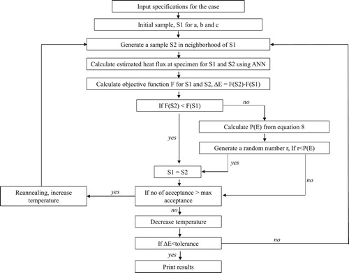
To obtain the optimum value of the heat flux control parameters following Equation (6(6) $F(\zeta )=min(\sum _i(q_{desired}-q_{estimated,i}(\zeta ){)}^2)$(6) ), we use the Simulated Annealing (SA) algorithm [39]. Simulated annealing is a non-traditional stochastic search technique, which derives its principles from slow cooling of metals (or annealing) used in metallurgy. As the metal is in hot state initially, its atoms are free to transit to a higher energy state, however, as the temperature of the metal reduces, the chance that an energy state would be changed further becomes smaller and smaller. Furthermore, it is desired to make all the atoms acquire a desired energy state, in general the crystalline state, which ensures better uniformity of the metal properties. To achieve this, the cooling rate (or temperature) should be controlled in an effective manner. The probabilistic distribution of energy states at a temperature T, when system is in equilibrium is given by Boltzmann's distribution, (7) $P(E)={\mathrm{e}}^{-E/kT}$(7) Here $P(E)$ is the probability distribution of energy states at temperature T and k is Boltzmann constant. It can be seen that, as T is higher the atoms will have a higher probability to acquire any energy state, while as T becomes lower, this probability also reduces. Analogous to this concept, in an optimization problem, initially the generated samples are allowed to explore a wider solution space but as the iterations progress, the exploration space becomes smaller and smaller. In other words, the extent of leap from one sample to the another becomes shorter. If we define $\mathrm{\Delta }E$ as the change in objective function value for a present sample and a newly generated sample, the Boltzmann equation can be used to determine the probability associated with accepting or rejecting this new sample. More precisely, the equation can be recast as, (8) $P(E)={\mathrm{e}}^{-\mathrm{\Delta }E/kT}$(8) Where T can be user-defined temperature to control the cooling. Therefore, by controlling the temperature effectively, one can ensure that the search converges to a state of minimum energy (or minimum value of objective function) as defined for a minimization problem. SA is a robust tool for handling optimization problems with varying degree of complexity. Furthermore, its extension to multiple variable optimization problem is straightforward. However, in order to avoid the algorithm trapping in a local minimum, reannealing is performed where the cooling rate is tweaked after a certain number of acceptances have taken place. In the present study, a MATLAB [38] based simulated annealing tool has been utilized and coupled with generated neural network to obtain the optimum values of a, b and c. The temperature for cooling in SA is controlled by expression $T=T_0\ast {0.95}^k$, where $T_0$ is initial temperature and k is annealing parameter which is similar to iteration number until reannealing condition is met. Number of acceptances before reannealing is set to 100. The algorithm stops when the difference in objective function value in subsequent iterations in less than 1E-06. The procedure of coupling the ANN solution with SA is presented in Figure 9.

Figure 9. Flowchart of the procedure of obtaining optimum values of a, b and c using ANN-SA algorithm.

7.2. Optimum values of heat flux control parameters and their validation

Following the algorithm mentioned in Figure 9, the optimum values of the heat flux control parameters a, b and c have been determined for the first and second design case (see Table 5) and the corresponding results are shown Table 6. The value of objective function indicates that the flux values are relatively close to the desired uniform flux. The computational time taken by the ANN-SA algorithm as mentioned in the last column of the Table 6 clearly indicates the fastness of this inverse technique. The optimum profiles of the non-dimensional heat flux input have been drawn for these two design cases as shown in Figure 10. In the next sections, further analysis on the effect of parameters such as specimen temperature, specimen emissivity and gas concentration on the obtained results has been performed.

Table 6. Optimum values of a, b and c as obtained from ANN-SA algorithm and corresponding computational time for the design cases mentioned in Table 5.

case	$q_d$	$T_{des}$	${ϵ}_d$	$Y_{\mathrm{H}2\mathrm{O}}$	a	b	c	F	time taken (s)
1st	$-4$	400	0.5	0.1	0.6079	0.4602	0.2310	0.0492	3.49
2nd	$-8$	400	0.5	0.1	0.8587	0.4798	0.6298	0.2121	2.72

Figure 10. Optimum profiles of heat input over the heater surface as obtained from the ANN-SA algorithm for the two design cases discussed in Table 5.

7.3. Effect of specimen temperature, emissivity and gas concentration

To assess the effect of specimen temperature and emissivity, different variants of design cases have been generated by changing the specimen surface temperature to $T_{des}=500\mathrm{K}$ and $T_{des}=300\mathrm{K}$ and specimen surface emissivity to $ϵ=0.25$ and $ϵ=0.75$. The optimums have also been obtained by changing the medium properties, where the ${\mathrm{H}}_2\mathrm{O}$ gas concentration is changed to $Y_{\mathrm{H}2\mathrm{O}}=0.05$ and $Y_{\mathrm{H}2\mathrm{O}}=0.2$. This generates a total of 6 variant cases for each design case. These cases have been listed in Table 7 for a uniform desired flux of $-4{\mathrm{kW}/\mathrm{m}}^2$ and in Table 8 for uniform desired flux of $-8{\mathrm{kW}/\mathrm{m}}^2$. The optimum values of a, b and c for these cases are determined from the ANN-SA algorithm have all been reported along with their objective function values. The maximum deviation in the values of local heat fluxes when compared to the desired flux ($q_d$) is calculated for all cases to assess the uniformity of the flux distribution. The last column of the tables report the validation results for the optimum, where the optimum values of a, b and c obtained for different cases have been used as an input to the forward RTE model and the difference in the values predicted by RTE and ANN is examined. The results are reported in terms of maximum deviation in local heat flux values between ANN and RTE at the optimum values of a, b and c. The results indicate that the deviations are really small for both the analysis (of the order of ${10}^{-2}{\mathrm{kW}/\mathrm{m}}^2$).

Table 7. Results of ANN-SA algorithm for the variants of design case corresponding to $q_d=-4{\mathrm{kW}/\mathrm{m}}^2$ by varying specimen temperature, emissivity and gas concentrations.

				Optimum values			Obj. function value
$q_d({\mathrm{kW}/\mathrm{m}}^2)$	$T_{des}(\mathrm{K})$	${ϵ}_d$	$Y_{\mathrm{H}2\mathrm{O}}$	a	b	c	F	$max$ $(|q_d-q_{ann,i}|)$	$max$ $(|q_{rte,i}-q_{ann,i}|)$
$-4$	500	0.5	0.1	0.4370	0.4018	0.3970	0.0513	0.1291	0.0626
$-4$	300	0.5	0.1	0.4960	0.3746	0.3223	0.0474	0.1326	0.0872
$-4$	400	0.25	0.1	0.7806	0.4730	0.1727	0.0120	0.0662	0.0376
$-4$	400	0.75	0.1	0.4620	0.3755	0.3689	0.1028	0.1777	0.0976
$-4$	400	0.5	0.2	0.3945	0.3066	0.5682	0.0534	0.1259	0.0119
$-4$	400	0.5	0.05	0.6605	0.4673	0.2085	0.0488	0.1338	0.0721

Table 8. Results of ANN-SA algorithm for the variants of design case corresponding to $q_d=-8{\mathrm{kW}/\mathrm{m}}^2$ by varying specimen temperature, emissivity and gas concentrations.

				Optimum values			Obj. function value
$q_d({\mathrm{kW}/\mathrm{m}}^2)$	$T_{des}(\mathrm{K})$	${ϵ}_d$	$Y_{\mathrm{H}2\mathrm{O}}$	a	b	c	F	$max$ $(|q_d-q_{ann,i}|)$	$max$ $(|q_{rte,i}-q_{ann,i}|)$
$-8$	500	0.5	0.1	0.8926	0.3010	0.6344	0.2130	0.2766	0.0298
$-8$	300	0.5	0.1	0.8624	0.4737	0.6269	0.2156	0.2727	0.0369
$-8$	400	0.25	0.1	0.8494	0.4457	0.6895	0.0549	0.1330	0.0137
$-8$	400	0.75	0.1	0.9106	0.5094	0.4893	0.4634	0.3810	0.0225
$-8$	400	0.5	0.2	0.8820	0.5822	0.5842	0.2250	0.2598	0.0369
$-8$	400	0.5	0.05	0.8875	0.5843	0.5740	0.2108	0.2507	0.0445

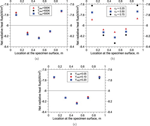
Next, the local heat fluxes at the specimen surface corresponding to the input heat flux profiles governed by the optimums given in Tables 7 and 8 have been obtained. The local heat flux values are then compared with the desired heat flux values ($q_d$) and the results of this analysis for $q_d=-4{\mathrm{kW}/\mathrm{m}}^2$ and $q_d=-8{\mathrm{kW}/\mathrm{m}}^2$ are plotted in Figures 11 and 12 respectively. The Figures 11(a) and 12(a) show the local flux values and their closeness to desired flux values on varying the specimen temperature ($T_{des}$), Figures 11(b) and 12(b) represent the similar effect on varying the specimen emissivity (${ϵ}_d$), and Figures 11(c) and 12(c) show this effect on varying the ${\mathrm{H}}_2\mathrm{O}$ gas concentrations. From the figures, it is clear that the obtained heat fluxes are very close to the desired ones for all the cases and this suggests that the present solution technique is accurate enough when applied to variety of test cases. It is also observed that as the desired heat flux increases it becomes more difficult to maintain the heat flux uniformity at any given specimen temperature. Moreover, at every desired heat flux level, a specimen with lower emissivity can ensure better heat flux uniformity. This is due to the fact that net radiative heat flux depends on the emission in an additive way and to the incident heat fluxes in a subtractive way. For higher emitting specimens the contribution due to emission is larger and because of adiabatic side walls more radiation is incident on the specimen. The region of the specimen close to adiabatic side walls receives more incident radiation due to shorter path lengths of rays emanating from the walls and hence shows a lower value of net radiation heat flux. Therefore, this appears to be difficult to obtain uniform heat fluxes over the specimen parts which are close to the side walls compared to the specimen parts located at the centre of the enclosure.

Figure 11. Values of net radiative fluxes at monitored locations on specimen surface for the first design case (i.e. $q_d=-4{\mathrm{kW}/\mathrm{m}}^2$) under the effect of (a) various specimen temperatures, (b) various specimen surface emissivities and (c) various ${\mathrm{H}}_2\mathrm{O}$ gas concentration.

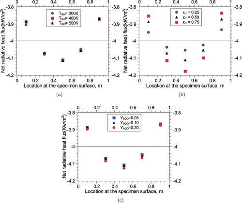
Figure 12. Values of net radiative fluxes at monitored locations on specimen surface for the first design case (i.e. $q_d=-8{\mathrm{kW}/\mathrm{m}}^2$) under the effect of (a) various specimen temperatures, (b) various specimen surface emissivities and (c) various ${\mathrm{H}}_2\mathrm{O}$ gas concentration.

7.4. Sensitivity analysis of the obtained optima

The optimum values of the control parameters obtained should be tested for their sensitivity. It is interesting to highlight that upon performing an exhaustive search for a design case, we find that there exist around 0.7% (7 in every 100) combination of values of control parameters which provide the objective function value fairly close to the minimum. It means that there exist not one but few combination of values of a, b and c which would provide objective function values close to global minima for this problem. However, the efficacy of an engineering algorithm is to provide a good workable solution that can be used practically. Nevertheless, from the obtained values, it was also verified that the present ANN-SA algorithm give values very close to the global optimum. In order to test the sensitivity and to obtain a confidence that the optimum values indicate a objective function value close to global minima, the optimum values of a, b and c have been varied with 5% random perturbation around the design case. The change in objective function value is then estimated using the surrogate model for these newly generated cases after perturbation. The results are shown in Table 9. From the table, it is observable that under such minute perturbation also the objective function values change considerably, which clearly indicates that the calculated optimums truly indicate minimum value of the objective function and hence confirms the credibility of the present results.

Table 9. Results of varying the optimum configuration by 5% random normal perturbation around the design case corresponding to $q_d=-4{\mathrm{kW}/\mathrm{m}}^2$.

$q_d$	a	b	c	$T_{des}$	${ϵ}_d$	$Y_{\mathrm{H}2\mathrm{O}}$	F
−4	0.6079	0.4602	0.2310	400	0.5	0.1	0.0492
$-4$	0.627	0.391	0.221	400	0.5	0.1	0.0684
$-4$	0.607	0.501	0.194	400	0.5	0.1	0.7278
$-4$	0.576	0.419	0.142	400	0.5	0.1	8.2503
$-4$	0.611	0.476	0.191	400	0.5	0.1	0.9161
$-4$	0.560	0.401	0.221	400	0.5	0.1	0.8056
$-4$	0.661	0.319	0.118	400	0.5	0.1	10.5483

8. Conclusions

An ANN-SA based inverse solution technique has been developed for obtaining the optimum heat source control parameters in a two dimensional radiant furnace. The FVM-SLW based radiative transfer solver has been utilized to generate the data for the training of the neural network. The trained networks were thoroughly compared and tested with the unseen data in order to avoid overfitting scenarios. The selected network was then coupled with simulated annealing (SA) algorithm to solve the inverse problem of estimating optimum heat source control parameters for a radiant furnace test case. The applicability of the method is discussed by choosing pseudo design cases and the role of other operation variables such as specimen temperature, specimen emissivity and gas concentration has been studied. The corresponding optimums have been obtained for the two design cases and their all possible variants. The sensitivity study of the obtained optimum values was also performed by introducing 5% random normal perturbation. Results have shown that ANN gives accurate estimation of the fluxes when compared with RTE and maximum errors were less than 6% for such predictions. Furthermore, ANN proves to be a fast estimation tool and serves as a potential surrogate to be used in such inverse problems. The optimum control parameters and the obtained fluxes show minimal dependence on specimen temperature and gas concentration, however emissivity of the specimen tend to effect the uniformity of the fluxes to a considerable extent. The uniformity is more difficult to maintain on a longer specimen and for a high value of desired heat fluxes. The cross validation results of the optima show a remarkable closeness in heat flux values obtained using ANN and RTE with the same optimums. The observed differences were of the order of ${10}^{-2}{\mathrm{kW}/\mathrm{m}}^2$. This gives good credibility on the predictions of the present network and its coupling with SA. Moreover, sensitivity analysis also confirms that for the present problem, combined ANN-SA technique gives results close to global minimum. Thus, the combined ANN-SA technique proves to be an efficient tool in fast and accurate estimation of the optimum parameters in a heat source optimization problem.

Nomenclature

a	=	control parameter related to peak value of heat flux
b	=	control parameter related to location of peak value of heat flux
c	=	control parameter related to spread of the flux distribution
F	=	objective function
$I_{\lambda }$	=	spectral intensity, W/m2sr μm
$I_{b\lambda }$	=	blackbody intensity, W/m2sr μm
k	=	Boltzmann constant
L	=	mean beam length of the enclosure
MSE	=	mean squared error
NGG	=	number of gray gases in SLW model
$Q_h$	=	heater power, W
$n_w$	=	unit normal at the wall
q	=	radiative heat flux, kW/m2
R	=	goodness of fit
T	=	Temperature, K
$u_j$	=	weight of the $j\mathrm{th}$ gray gas in SLW model
x	=	inputs to the neural network
Y	=	gas specie mole fraction

Greek symbols

ε	=	emissivity
${\kappa }_j$	=	absorption coefficient of $j\mathrm{th}$ gray gas in SLW model, m-1
$\mu ,\eta$	=	direction cosines

Subscripts

ann	=	ANN estimated values
d	=	specimen related quantities
g	=	gas properties
h	=	heater related quantities
i	=	location index at specimen surface
j	=	$j\mathrm{th}$ gray gas
λ	=	wavelength dependent quantities
m	=	input index in the network
n	=	neuron index in the network
rte	=	RTE estimated values

Disclosure statement

No potential conflict of interest was reported by the authors.

References

- Baik O, Marcotte M, Castaigne F. Cake baking in tunnel type multi-zone industrial ovens part I. Characterization of baking conditions. Food Res Int. 2000;33(7):587–598. doi: 10.1016/S0963-9969(00)00095-8
- Zhang H, Deng S. Evaluating heat flux profiles in aluminum reheating furnace with regenerative burner. Energies. 2017;10(4):562. doi: 10.3390/en10040562
- Franca F, Morales JC, Oguma M, et al. Inverse radiation heat transfer within enclosures with nonisothermal participating media. In: International Heat Transfer Conference, Kyongju, Korea; Vol. 7; 1998. p. 433–438.
- Berrocal Tito MJ, Roberty NC, Silva Neto AJ, et al. Inverse radiative transfer problems in two-dimensional participating media. Inverse Probl Sci Eng. 2004;12(1):103–121. doi: 10.1080/10682760310001597536
- Howell J, Ezekoye O, Morales J. Inverse design model for radiative heat transfer. J Heat Transfer. 2000;122(3):492–502. doi: 10.1115/1.1288774
- Rukolaine S. Regularization of inverse boundary design radiative heat transfer problems. J Quant Spectros Radiat Transf. 2007;104(1):171–195. doi: 10.1016/j.jqsrt.2006.09.001
- Das MK, Tariq A, Panigrahi PK, et al. Estimation of convective heat transfer coefficient from transient liquid crystal data using an inverse technique. Inverse Probl Sci Eng. 2005;13(2):133–155. doi: 10.1080/10682760412331313414
- França FH, Howell JR, Ezekoye OA, et al. Inverse design of thermal systems with dominant radiative transfer. In: Advances in heat transfer. Vol. 36. Elsevier, Massachusetts, United States; 2003. p. 1–110.
- Daun K, França F, Larsen M, et al. Comparison of methods for inverse design of radiant enclosures. J Heat Transfer. 2006;128(3):269–282. doi: 10.1115/1.2151198
- Schneider PS, Mossi AC, França FHR, et al. Application of inverse analysis to illumination design. Inverse Probl Sci Eng. 2009;17(6):737–753. doi: 10.1080/17415970802522380
- Lemos LD, Brittes R, França FH. Application of inverse analysis to determine the geometric configuration of filament heaters for uniform heating. Int J Therm Sci. 2016;105:1–12. doi: 10.1016/j.ijthermalsci.2016.02.015
- Kim KW, Baek SW, Kim MY, et al. Estimation of emissivities in a two-dimensional irregular geometry by inverse radiation analysis using hybrid genetic algorithm. J Quant Spectrosc Radiat Transf. 2004;87(1):1–14. doi: 10.1016/j.jqsrt.2003.08.012
- Kim KW, Baek SW. Inverse surface radiation analysis in an axisymmetric cylindrical enclosure using a hybrid genetic algorithm. Numer Heat Transf Part A. 2004;46(4):367–381. doi: 10.1080/10407780490478533
- Safavinejad A, Maruyama S, Mansouri SH, et al. Optimal boundary design of radiant enclosures using micro-genetic algorithm. J Therm Sci Technol. 2008;3(2):179–194. doi: 10.1299/jtst.3.179
- Safavinejad A, Mansouri S, Sakurai A, et al. Optimal number and location of heaters in 2-d radiant enclosures composed of specular and diffuse surfaces using micro-genetic algorithm. Appl Therm Eng. 2009;29(5–6):1075–1085. doi: 10.1016/j.applthermaleng.2008.05.025
- Amiri H, Mansouri SH, Safavinejad A, et al. The optimal number and location of discrete radiant heaters in enclosures with the participating media using the micro genetic algorithm. Numer Heat Transf Part A. 2011;60(5):461–483. doi: 10.1080/10407782.2011.600597
- Payan S, Farahmand A, Sarvari SH. Inverse boundary design radiation problem with radiative equilibrium in combustion enclosures with pso algorithm. Int Commun Heat Mass Transf. 2015;68:150–157. doi: 10.1016/j.icheatmasstransfer.2015.08.009
- Sun S, Qi H, Zhao F, et al. Inverse geometry design of two-dimensional complex radiative enclosures using krill herd optimization algorithm. Appl Therm Eng. 2016;98:1104–1115. doi: 10.1016/j.applthermaleng.2016.01.017
- Queipo NV, Haftka RT, Shyy W, et al. Surrogate-based analysis and optimization. Prog Aerosp Sci. 2005;41(1):1–28. doi: 10.1016/j.paerosci.2005.02.001
- Howell JR, Daun K, Erturk H, et al. The use of inverse methods for the design and control of radiant sources. JSME Int J Ser B Fluids Therm Eng. 2003;46(4):470–478. doi: 10.1299/jsmeb.46.470
- Yuen WW. RAD-NNET, a neural network based correlation developed for a realistic simulation of the non-gray radiative heat transfer effect in three-dimensional gas-particle mixtures. Int J Heat Mass Transf. 2009;52(13–14):3159–3168. doi: 10.1016/j.ijheatmasstransfer.2009.01.041
- Yuen W, Tam W, Chow W. Assessment of radiative heat transfer characteristics of a combustion mixture in a three-dimensional enclosure using RAD-NETT (with application to a fire resistance test furnace). Int J Heat Mass Transf. 2014;68:383–390. doi: 10.1016/j.ijheatmasstransfer.2013.08.009
- Yadav R, Balaji C, Venkateshan S. Inverse estimation of number and location of discrete heaters in radiant furnaces using artificial neural networks and genetic algorithm. J Quant Spectrosc Radiat Transf. 2019;226:127–137. doi: 10.1016/j.jqsrt.2018.12.031
- Chai JC, Lee HS, Patankar SV. Finite volume method for radiation heat transfer. J Thermophys Heat Transf. 1994;8(3):419–425. doi: 10.2514/3.559
- Denison MK, Webb BW. A spectral line-based weighted-sum-of-gray-gases model for arbitrary RTE solvers. J Heat Transfer. 1993;115(4):1004–1012. doi: 10.1115/1.2911354
- Yadav R, Chakravarthy B, Venkateshan S. Implementation of SLW model in the radiative heat transfer problems with particles and high temperature gradients. Int J Numer Methods Heat Fluid Flow. 2017;27(5):1128–1141. doi: 10.1108/HFF-03-2016-0095
- Denison M, Webb BW. An absorption-line blackbody distribution function for efficient calculation of total gas radiative transfer. J Quant Spectrosc Radiat Transf. 1993;50(5):499–510. doi: 10.1016/0022-4073(93)90043-H
- Solovjov VP, Webb BW. SLW modeling of radiative transfer in multicomponent gas mixtures. J Quant Spectrosc Radiat Transf. 2000;65(4):655–672. doi: 10.1016/S0022-4073(99)00133-8
- Amiri H, Lari K. Comparison of global radiative models in two-dimensional enclosures at radiative equilibrium. Int J Therm Sci. 2016;104:423–436. doi: 10.1016/j.ijthermalsci.2016.01.020
- Levenberg K. A method for the solution of certain non-linear problems in least squares. Quart Appl Math. 1944;2(2):164–168. doi: 10.1090/qam/10666
- Møller MF. A scaled conjugate gradient algorithm for fast supervised learning. Neural Netw. 1993;6(4):525–533. doi: 10.1016/S0893-6080(05)80056-5
- MacKay DJ. Bayesian interpolation. Neural Comput. 1992;4(3):415–447. doi: 10.1162/neco.1992.4.3.415
- Lenis YA, Maag G, de Oliveira CEL, et al. Effect of heat flux distribution profile on hydrogen concentration in an allothermal downdraft biomass gasification process: modeling study. J Energy Resour Technol. 2019;141(3): 031801, 1–10. doi: 10.1115/1.4041723
- Lockwood F, Shah N. A new radiation solution method for incorporation in general combustion prediction procedures. In: Symposium (International) on Combustion; Vol. 18. London: Elsevier; 1981. p. 1405–1414.
- Jamaluddin A, Smith P. Predicting radiative transfer in axisymmetric cylindrical enclosures using the discrete ordinates method. Combust Sci Technol. 1988;62(4–6):173–186. doi: 10.1080/00102208808924008
- ANSYS. Version 14.0. Cannonsburg: ANSYS Inc.; 2014.
- McKay MD, Beckman RJ, Conover WJ. Comparison of three methods for selecting values of input variables in the analysis of output from a computer code. Technometrics. 1979;21(2):239–245.
- MATLAB. Version 8.3.0 (R2014a). Natick (MA): The MathWorks Inc.; 2014.
- Ingber L. Adaptive simulated annealing (ASA): lessons learned. Control Cybernet. 1996;25(1):33–54.