A numerical scheme based on discrete mollification method using Bernstein basis polynomials for solving the inverse one-dimensional Stefan problem

ABSTRACT

This paper concerns a one-phase inverse Stefan problem in one-dimensional space. The problem is ill-posed in the sense that the solution does not depend continuously on the data. We also consider noisy data for this problem. As such, we first regularize the proposed problem by the discrete mollification method. We apply the integration matrix using Bernstein basis polynomials for the discrete mollification method. Through this method, the execution time was gradually decreased. We then extend the space marching algorithm for solving our problem. Moreover, proofs of stability and convergence of the process are given. Finally, the results of this paper have been illustrated and examined by some numerical examples. Numerical examples confirm the efficiency of the proposed method.

Keywords:

• One-phase inverse Stefan problem
• discrete mollification
• Bernstein basis polynomials
• space marching algorithm
• stability
• convergence

2010 Mathematics Subject Classifications:

• 35R30
• 35R37
• 80A22

1. Introduction

The term ‘Stefan problem’ is generally used for problems with phase-changes such as from the liquid to the solid. Stefan problem has piqued increasing interest of many researchers for over a century, since these problems are important in many engineering, science and technology applications such as freezing the foodstuffs [1], crystal growth [2,3], solidification and melting of metals [4,5], laser drilling in metals and the cornea [6], the surgical removal of a body part or tissue, such as in atrial fibrillation [7], movement of sea coasts with the ocean depth and a surface flux changing as a power of time [8,9], preservation of human blood, solar energy storage [10] and many others.

The direct Stefan problem consists of determining the temperature in the domain and the position of the moving interface when the initial and boundary conditions, and the thermal properties of the heat conducting body are known [10–15]. One class of inverse Stefan problem requires the reconstruction of the function which describes the boundary conditions when the position of the moving boundary is known [16]. This kind of problem becomes an inverse design problem [17]. Moreover, inverse Stefan problems belong to a very important class of improperly posed problems in control theory which have many engineering applications. For example, in the technology of refining a material by means of recrystallization, one is interested in solving the inverse Stefan problem which consists of finding the temperature and heat flux at the fixed surface guaranteeing the flatness of the crystallization front [18].

The exact or analytic solutions of direct and inverse Stefan problems are restricted to a few simple cases. One often has to apply numerical methods such as the finite difference method [19], the boundary element method (BEM) [20], the method of fundamental solutions [18], the heat balance integral method and the refined integral method [21], the variational iteration method [17], etc. in solving these phase-change problems. Here, we propose a stable and convergent numerical algorithm based on the discrete mollification and space marching methods for solving a one-phase inverse Stefan problem. The mollification method is recognized as a reliable and capable regularization method that has been widely applied to solve many ill-posed problems [22–25]. It uses a convolution of the noisy data and a specific function with a parameter to smooth the noisy data. More recently, it has been proved that the mollification method is a versatile and useful tool when dealing with parabolic partial differential equations [22,25]. Simple implementation, accurate and stable solution in the presence of high level noise is the main characteristic of the mollification method. In this paper, we introduce a new discrete mollification method based on the integration matrix using Bernstein basis polynomials.

The outline of this paper is as follows. In Section 2, we formulate the direct and inverse Stefan problems. Section 3 begins with a brief description of the discrete mollification method followed by a new approach for it based on the integration matrix using Bernstein basis polynomials. In Section 4, we regularize and solve our inverse Stefan problem. Section 5 concerns the stability and convergence proof of the space marching numerical algorithm. Finally, some numerical examples are given in Section 6. The numerical results show that an accurate and computationally low-cost approximation to the inverse Stefan problem can be obtained using the presented method.

2. Mathematical model

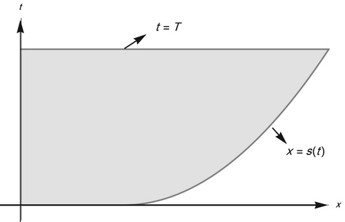
Let $D=\{(x,t);t\in (0,T),x\in (0,s(t))\}$ be a domain in ${\mathbb{R}}^2$ (Figure 1). For the direct one-phase Stefan problem we seek a solution $(u(x,t),s(t))$ which satisfies the following equation (1) $u_t(x,t)=\alpha u_{xx}(x,t),(x,t)\in D,$(1) subject to the initial condition (2) $u(x,0)=\phi (x),x\in [0,s(0)],s(0)>0,$(2) the Dirichlet and Neumann boundary conditions on the moving boundary $x=s(t)$ (3) $\begin{array}{rl}u(s(t),t)& =g_1(t),t\in [0,T],\end{array}$(3) (4) $\begin{array}{rl}{u}_x(s(t),t)& =g_2(t),t\in [0,T]\end{array}$(4) and Dirichlet boundary condition on x = 0 (5) $u(0,t)=q(t),t\in [0,T]$(5) (for more details, see [17]), where α is the thermal diffusivity, $g_1(t)=0$ and $g_2(t)=-k{s}^{\prime }(t)$, with $k=\rho L/K$, ρ is the density, L is the latent heat and K is the thermal conductivity, T is a given final time, $s(t)\in C^1([0,T])$ is a positive nondecreasing function describing the position of the moving boundary, $\phi (x)\in C^1([0,s(0)])$ is given and u, x and t refer to temperature, space and time, respectively. The boundary condition in (5(5) $u(0,t)=q(t),t\in [0,T]$(5) ) can be changed to the (6) $u_x(0,t)=p(t),t\in [0,T].$(6)

Figure 1. Domain representation of the one-phase Stefan problem.

Existence and uniqueness of a solution, and continuous dependence on the data, i.e. well-posedness, for $u(x,t)$ and $s(t)$ hold for the direct one-phase Stefan problem (1(1) $u_t(x,t)=\alpha u_{xx}(x,t),(x,t)\in D,$(1) )–(5(5) $u(0,t)=q(t),t\in [0,T]$(5) ) and (1(1) $u_t(x,t)=\alpha u_{xx}(x,t),(x,t)\in D,$(1) )–(4(4) $\begin{array}{rl}{u}_x(s(t),t)& =g_2(t),t\in [0,T]\end{array}$(4) ),(6(6) $u_x(0,t)=p(t),t\in [0,T].$(6) ) [10,26,27]. The inverse Stefan problem that will be considered in this paper consists of finding the temperature $u(x,t)$, $q(t)$ and $p(t)$ satisfying (1(1) $u_t(x,t)=\alpha u_{xx}(x,t),(x,t)\in D,$(1) )–(6(6) $u_x(0,t)=p(t),t\in [0,T].$(6) ), when the moving boundary $s(t)$ is known. This inverse problem is highly ill-posed [26]. Now, we assume that functions $\phi (x)$ and $g_2(t)$ are not known exactly and we only have approximations of these functions presented as ${\phi }^{\epsilon }(x)$ and $g_2^{\epsilon }(t)$, respectively. In addition, these approximate functions satisfy the following conditions: $\begin{array}{rl}& {\Vert \phi (x)-{\phi }^{\epsilon }(x)\Vert }_{\mathrm{\infty }}\le \epsilon ,\\ & {\Vert g_2(t)-g_2^{\epsilon }(t)\Vert }_{\mathrm{\infty }}\le \epsilon ,\end{array}$ where ϵ denotes the maximum level of noise. Due to perturbations in the problem's data and the ill-posedness of the proposed problem, we first regularize the problem through a method called discrete mollification.

In the next section, we introduce a new discrete mollification method based on Bernstein basis polynomials.

3. The method of discrete mollification using Bernstein basis polynomials

Mollification is a filtering procedure, based on convolution, which has proven to be convenient for the regularization of a variety of ill-posed problems [22–25,28,29]. In this section, we first recall the definition of Bernstein polynomials and using these polynomials, we find the integration matrix in this basis. Next, we introduce the basic idea of our new discrete mollification method based on the mentioned integration matrix.

3.1. Bernstein basis polynomials and the integral matrix

A Bernstein polynomial (also called Bézier polynomial) defined over the interval $[a,b]$ has the form (7) $b_{j,M}(x)=(\genfrac{}{}{0ex}{}{M}{j})\frac{{(x-a)}^j{(b-x)}^{M-j}}{{(b-a)}^M},j=0,\dots ,M.$(7) This is not a typical scaling of the Bernstein polynomials; however, this scaling makes matrix notations related to this basis slightly easier to write.

We choose Bernstein basis polynomials because when $M\to \mathrm{\infty }$, Bernstein polynomials are appropriate and reasonable approximations to functions involved in the mollification process. Moreover, the integration matrix for Bernstein basis polynomials is well structured and easy to use. This enables us to take the integrals quickly and efficiently which substantially reduces the necessary CPU times (see Tables 1 and 2).

Table 1. RMS and CPU time(s) for $g(t)$ in Example 6.1.

ϵ	N	RMS for new technique	RMS for old technique	CPU time(s) for new technique	CPU time(s) for old technique
0.001	100	0.000423465	0.000479141	0.280802	6.02164
0.001	150	0.000393147	0.000478458	0.608126	9.00126
0.001	200	0.000373714	0.000430193	0.998406	12.2773

Table 2. RMS for $g(t)$ in Example 6.2.

ϵ	N	RMS for new technique	RMS for old technique [25]
0.00	128	0.00032	0.00049
0.05	128	0.01032	0.01555
0.10	128	0.01855	0.03249
0.00	256	0.00010	0.00014
0.05	256	0.00915	0.01398
0.10	256	0.01694	0.03773

The Bernstein polynomials are nonnegative in $[a,b]$, i.e. $b_{j,M}(x)\ge 0$ for all $x\in [a,b]$ $(j=0,\dots ,M).$ Bernstein polynomials are widely used in computer-aided geometric design [30].

For a function $f(x)\in C[a,b]$, a polynomial approximation, $P(x)$, written using Bernstein basis is of the form (8) $P(x)=\sum _{j=0}^M{a}_j{b}_{j,M}(x)=\left[\begin{array}{ccccc}{a}_0& a_1& \dots & a_{M-1}& a_M\end{array}\right]\mathbf{I}\left[\begin{array}{c}{b}_{0,M}(x)\\ b_{1,M}(x)\\ ⋮\\ b_{M-1,M}(x)\\ b_{M,M}(x)\end{array}\right],$(8) where the $a_j$'s are sometimes called the Bézier coefficients $(j=0,\dots ,M)$ and are defined by: $a_j=f(a+\frac{(b-a)j}{M}).$

Lemma 3.1

If $P(x)$ is given by (8(8) $P(x)=\sum _{j=0}^M{a}_j{b}_{j,M}(x)=\left[\begin{array}{ccccc}{a}_0& a_1& \dots & a_{M-1}& a_M\end{array}\right]\mathbf{I}\left[\begin{array}{c}{b}_{0,M}(x)\\ b_{1,M}(x)\\ ⋮\\ b_{M-1,M}(x)\\ b_{M,M}(x)\end{array}\right],$(8) ), then (9) $\int P(x)\mathrm{d}x=(\mathbf{c}+\left[\begin{array}{ccccc}{a}_0& a_1& \dots & a_{M-1}& a_M\end{array}\right]\mathbf{A})\left[\begin{array}{c}{b}_{0,M+1}(x)\\ b_{1,M+1}(x)\\ ⋮\\ b_{M,M+1}(x)\\ b_{M+1,M+1}(x)\end{array}\right],$(9) where $\mathbf{c}=\left[\begin{array}{ccccc}c& c& \dots & c& c\end{array}\right]$ is an undetermined constant row vector of size M + 2 and $\mathbf{A}$ is an $(M+1)\times (M+2)$ matrix that has the following structure: (10) $A_{i,j}=\{\begin{array}{ll}{\displaystyle \frac{a-b}{M+1}},& i=j=1,\\ 0,& i=1;j>1,\\ {\displaystyle \frac{1}{M+1}}{\displaystyle \frac{\sum _{k=0}^{M+1-i}(\genfrac{}{}{0ex}{}{M+1}{k}){(-1)}^k{a}^{M+1-k}{b}^k}{{(a-b)}^M}},& 1<i<M+1;i\ge j,\\ -{\displaystyle \frac{1}{M+1}}{\displaystyle \frac{\sum _{k=M+2-i}^{M+1}(\genfrac{}{}{0ex}{}{M+1}{k}){(-1)}^k{a}^{M+1-k}{b}^k}{{(a-b)}^M}},& 1<i<M+1;i<j,\\ 0,& i=M+1;j<M+2,\\ -{\displaystyle \frac{a-b}{M+1}},& i=M+1;j=M+2.\end{array}$(10)

Proof.

A little computation using (7(7) $b_{j,M}(x)=(\genfrac{}{}{0ex}{}{M}{j})\frac{{(x-a)}^j{(b-x)}^{M-j}}{{(b-a)}^M},j=0,\dots ,M.$(7) ) shows that [31] (11) $b_{k,M}^{\prime }(x)=\frac{k-1}{a-b}{b}_{k-1,M}(x)+\frac{M-2k}{a-b}{b}_{k,M}(x)+\frac{M-k}{a-b}{b}_{k+1,M}(x),k=0,1,\dots ,M,$(11) where any $b_{j,M}(x)$ with either a negative or larger than M index, j, is set to 0 in (11(11) $b_{k,M}^{\prime }(x)=\frac{k-1}{a-b}{b}_{k-1,M}(x)+\frac{M-2k}{a-b}{b}_{k,M}(x)+\frac{M-k}{a-b}{b}_{k+1,M}(x),k=0,1,\dots ,M,$(11) ). Now, we take the antiderivatives of the sides of (11(11) $b_{k,M}^{\prime }(x)=\frac{k-1}{a-b}{b}_{k-1,M}(x)+\frac{M-2k}{a-b}{b}_{k,M}(x)+\frac{M-k}{a-b}{b}_{k+1,M}(x),k=0,1,\dots ,M,$(11) ) for $k=0,1,\dots ,M$. We can then write the basis functions of degree M of the left-hand side of the resulting equation in terms of those of degree M + 1 (see e.g. [32] for more details) and from there, it is fairly easy to derive (10(10) $A_{i,j}=\{\begin{array}{ll}{\displaystyle \frac{a-b}{M+1}},& i=j=1,\\ 0,& i=1;j>1,\\ {\displaystyle \frac{1}{M+1}}{\displaystyle \frac{\sum _{k=0}^{M+1-i}(\genfrac{}{}{0ex}{}{M+1}{k}){(-1)}^k{a}^{M+1-k}{b}^k}{{(a-b)}^M}},& 1<i<M+1;i\ge j,\\ -{\displaystyle \frac{1}{M+1}}{\displaystyle \frac{\sum _{k=M+2-i}^{M+1}(\genfrac{}{}{0ex}{}{M+1}{k}){(-1)}^k{a}^{M+1-k}{b}^k}{{(a-b)}^M}},& 1<i<M+1;i<j,\\ 0,& i=M+1;j<M+2,\\ -{\displaystyle \frac{a-b}{M+1}},& i=M+1;j=M+2.\end{array}$(10) ). For example, for M = 3, $\mathbf{A}$ has the following form (12) $\begin{array}{rl}\mathbf{A}& =[\begin{array}{ccc}{\displaystyle \frac{a-b}{4}}& 0& 0\\ {\displaystyle \frac{1}{4}}{\displaystyle \frac{a^4-4a^{3}b+6a^2{b}^2}{{(a-b)}^3}}& {\displaystyle \frac{1}{4}}{\displaystyle \frac{a^4-4a^{3}b+6a^2{b}^2}{{(a-b)}^3}}& -{\displaystyle \frac{1}{4}}{\displaystyle \frac{b^4-4a{b}^3}{{(a-b)}^3}}\\ {\displaystyle \frac{1}{4}}{\displaystyle \frac{a^4-4a^{3}b}{{(a-b)}^3}}& {\displaystyle \frac{1}{4}}{\displaystyle \frac{a^4-4a^{3}b}{{(a-b)}^3}}& {\displaystyle \frac{1}{4}}{\displaystyle \frac{a^4-4a^{3}b}{{(a-b)}^3}}\\ 0& 0& 0\end{array}\\ & \begin{array}{cc}0& 0\\ -{\displaystyle \frac{1}{4}}{\displaystyle \frac{b^4-4a{b}^3}{{(a-b)}^3}}& -{\displaystyle \frac{1}{4}}{\displaystyle \frac{b^4-4a{b}^3}{{(a-b)}^3}}\\ -{\displaystyle \frac{1}{4}}{\displaystyle \frac{b^4-4a{b}^3+6a^2{b}^2}{{(a-b)}^3}}& -{\displaystyle \frac{1}{4}}{\displaystyle \frac{b^4-4a{b}^3+6a^2{b}^2}{{(a-b)}^3}}\\ 0& -{\displaystyle \frac{a-b}{4}}\end{array}].\end{array}$(12)

3.2. A new discrete mollification method

We first assume $G=\{g(x_j)=g_j{\}}_{j=0}^M$ to be a discrete function defined on $K=\{x_j,j=0,\dots ,M\}\subset I=[0,1]$ satisfying $0\le x_0<x_1<\cdots <x_{M-1}<x_M\le 1.$ In [25], for p>0 and every $x\in I_{\delta }=[p\delta ,1-p\delta ]$, Murio defined discrete mollification of G as follows. (13) $J_{\delta }G(x)=\sum _{j=0}^M({\int }_{{\alpha }_j}^{{\alpha }_{j+1}}{\rho }_{\delta ,p}(x-s)\mathrm{d}s)g_j,$(13) where ${\alpha }_0=0$, ${\alpha }_j=(x_j+x_{j+1})/2,j=1,\dots ,M$, ${\alpha }_{M+1}=1$ and ${\rho }_{\delta ,p}(x)=\{\begin{array}{ll}{A}_p{\delta }^{-1}\exp (-{\displaystyle \frac{x^2}{{\delta }^2}}),& \left|x\right|\le p\delta ,\\ 0,& \left|x\right|>p\delta ,\end{array}$ such that $A_p=({\int }_{-p}^p\exp (-s^2)\mathrm{d}s{)}^{-1}$. From now on, the p-dependency on the kernel has been dropped for simplicity of notation.

Now, let ${\mathbb{B}}_M[g(x)]=\sum _{j=0}^{M}g(j/M)b_{j,M}(x)$ be the degree-M Bernstein approximation of $g(x)$ over $[0,1]$. If $g\in C^r[0,1]$, r = 0, 1, we have the following result about the rate of convergence of ${\mathbb{B}}_M[g(x)]$ [33]: (14) $|{\mathbb{B}}_M[g(x)]-g(x)|\le C_r^{\ast }{M}^{-(r/2)}{\omega }_r(M^{-(1/2)}),$(14) where ${\omega }_r(M^{-(1/2)})$ is modulus of continuity of $g(x)$ and $C_r^{\ast }=(5-2r)/4$.

We define the discrete mollification of G through the integration matrix (10(10) $A_{i,j}=\{\begin{array}{ll}{\displaystyle \frac{a-b}{M+1}},& i=j=1,\\ 0,& i=1;j>1,\\ {\displaystyle \frac{1}{M+1}}{\displaystyle \frac{\sum _{k=0}^{M+1-i}(\genfrac{}{}{0ex}{}{M+1}{k}){(-1)}^k{a}^{M+1-k}{b}^k}{{(a-b)}^M}},& 1<i<M+1;i\ge j,\\ -{\displaystyle \frac{1}{M+1}}{\displaystyle \frac{\sum _{k=M+2-i}^{M+1}(\genfrac{}{}{0ex}{}{M+1}{k}){(-1)}^k{a}^{M+1-k}{b}^k}{{(a-b)}^M}},& 1<i<M+1;i<j,\\ 0,& i=M+1;j<M+2,\\ -{\displaystyle \frac{a-b}{M+1}},& i=M+1;j=M+2.\end{array}$(10) ) in the following form: (15) $\begin{array}{rl}{J}_{\delta }G(x)& ={\int }_0^1{\mathbb{B}}_M[{\rho }_{\delta }(x-s)g(s)]\mathrm{d}s\\ & ={\int }_0^1\left(\begin{array}{ccccc}{\rho }_{\delta }(x-s_0)g_0& {\rho }_{\delta }(x-s_1)g_1& \cdots & {\rho }_{\delta }(x-s_{M-1})g_{M-1}& {\rho }_{\delta }(x-s_M)g_M\end{array}\right)\\ & \mathbf{I}\left(\begin{array}{c}{b}_{0,M}(s)\\ b_{1,M}(s)\\ ⋮\\ b_{M-1,M}(s)\\ b_{M,M}(s)\end{array}\right)\mathrm{ds}\\ & =\left(\begin{array}{ccccc}{\rho }_{\delta }(x-s_0)g_0& {\rho }_{\delta }(x-s_1)g_1& \cdots & {\rho }_{\delta }(x-s_{M-1})g_{M-1}& {\rho }_{\delta }(x-s_M)g_M\end{array}\right)\\ & {\mathbf{A}\left(\begin{array}{c}{b}_{0,M+1}(s)\\ b_{1,M+1}(s)\\ ⋮\\ b_{M,M+1}(s)\\ b_{M+1,M+1}(s)\end{array}\right)|}_{s=0}^{s=1},\mathrm{for}x\in [p\delta ,1-p\delta ],\end{array}$(15) where $b_{j,M}$ and $\mathbf{A}$ are defined in Equations (7(7) $b_{j,M}(x)=(\genfrac{}{}{0ex}{}{M}{j})\frac{{(x-a)}^j{(b-x)}^{M-j}}{{(b-a)}^M},j=0,\dots ,M.$(7) ) and (10(10) $A_{i,j}=\{\begin{array}{ll}{\displaystyle \frac{a-b}{M+1}},& i=j=1,\\ 0,& i=1;j>1,\\ {\displaystyle \frac{1}{M+1}}{\displaystyle \frac{\sum _{k=0}^{M+1-i}(\genfrac{}{}{0ex}{}{M+1}{k}){(-1)}^k{a}^{M+1-k}{b}^k}{{(a-b)}^M}},& 1<i<M+1;i\ge j,\\ -{\displaystyle \frac{1}{M+1}}{\displaystyle \frac{\sum _{k=M+2-i}^{M+1}(\genfrac{}{}{0ex}{}{M+1}{k}){(-1)}^k{a}^{M+1-k}{b}^k}{{(a-b)}^M}},& 1<i<M+1;i<j,\\ 0,& i=M+1;j<M+2,\\ -{\displaystyle \frac{a-b}{M+1}},& i=M+1;j=M+2.\end{array}$(10) ), respectively.

Next, we obtain (16) $J_{\delta }G(x)=\frac{1}{M+1}\sum _{j=0}^M{\rho }_{\delta }(x-s_j)g_j.$(16) See Examples 6.1 and 6.2 of Section 6 for some numerical examples.

From now on, we refer to Equation (13(13) $J_{\delta }G(x)=\sum _{j=0}^M({\int }_{{\alpha }_j}^{{\alpha }_{j+1}}{\rho }_{\delta ,p}(x-s)\mathrm{d}s)g_j,$(13) ) and (16(16) $J_{\delta }G(x)=\frac{1}{M+1}\sum _{j=0}^M{\rho }_{\delta }(x-s_j)g_j.$(16) ) as the old and new techniques for discrete mollification, respectively. We usually take p = 3 and the radius of mollification, δ, is selected automatically by generalized cross validation method (GCV) (for more details, see [25]). The new technique for discrete mollification satisfies consistency, stability and convergence estimates as follows.

Theorem 3.2

Let $\mathrm{\Delta }x=|x_{j+1}-x_j|,j=0,\dots ,M-1$, $C_{\delta }^{\ast }$ and $C_{\delta }^{\prime }$ be the Lipschitz constants of ${\rho }_{\delta }(x-s)g(s)$ and $\mathrm{d}/\mathrm{d}x({\rho }_{\delta }(x-s)g(s)),$ respectively.

1. If $g(x)\in C^1(I)$ and $G=\{g(x_j)=g_j{\}}_{j=0}^M$ is the discrete version of g, then there exist positive constants C, $C_{\delta }^{\ast }$ and $C_{\delta }^{\prime }$ such that ${\Vert J_{\delta }G-g\Vert }_{\mathrm{\infty }}\le C\delta +\frac{3}{4}{C}_{\delta }^{\ast }\mathrm{\Delta }x.$ Moreover, if $g^{\prime }(x)\in C^1(I)$ then, ${\Vert {(J_{\delta }G)}^{\mathrm{\prime }}-g^{\mathrm{\prime }}\Vert }_{\mathrm{\infty }}\le C\delta +\frac{3}{4}{C}_{\delta }^{\prime }\mathrm{\Delta }x.$

2. If $G^{\epsilon }=\{g_j^{\epsilon }{\}}_{j=0}^M$ is the perturbed discrete version of g satisfying $\Vert G-G^{\epsilon }{\Vert }_{\mathrm{\infty },K}\le \epsilon ,$ then $\begin{array}{rl}& {\Vert J_{\delta }{G}^{\epsilon }-J_{\delta }G\Vert }_{\mathrm{\infty }}\le \frac{A_p}{\delta }\epsilon ,\\ & {\Vert (J_{\delta }{G}^{\epsilon }{)}^{\prime }-(J_{\delta }G{)}^{\prime }\Vert }_{\mathrm{\infty }}\le \frac{2p{A}_p}{{\delta }^2}\epsilon .\end{array}$

3. If $g(x)\in C^1(I)$ and $G^{\epsilon }=\{g_j^{\epsilon }{\}}_{j=0}^M$ is the perturbed discrete version of g satisfying $\Vert G-G^{\epsilon }{\Vert }_{\mathrm{\infty },K}\le \epsilon ,$ then there exist positive constants C, $C_{\delta }^{\ast }$ and $C_{\delta }^{\prime }$ such that $\begin{array}{rl}& {\Vert J_{\delta }{G}^{\epsilon }-J_{\delta }g\Vert }_{\mathrm{\infty }}\le \frac{A_p}{\delta }\epsilon +\frac{3}{4}{C}_{\delta }^{\ast }\mathrm{\Delta }x,\\ & {\Vert J_{\delta }{G}^{\epsilon }-g\Vert }_{\mathrm{\infty }}\le C\delta +\frac{A_p}{\delta }\epsilon +\frac{3}{4}{C}_{\delta }^{\ast }\mathrm{\Delta }x.\end{array}$ Moreover, if $g^{\prime }(x)\in C^1(I)$ then, $\begin{array}{rl}& {\Vert {(J_{\delta }{G}^{\epsilon })}^{\mathrm{\prime }}-{(J_{\delta }g)}^{\mathrm{\prime }}\Vert }_{\mathrm{\infty }}\le \frac{2p{A}_p}{{\delta }^2}\epsilon +\frac{3}{4}{C}_{\delta }^{\prime }\mathrm{\Delta }x,\\ & {\Vert {(J_{\delta }{G}^{\epsilon })}^{\mathrm{\prime }}-g^{\mathrm{\prime }}\Vert }_{\mathrm{\infty }}\le C\delta +\frac{2p{A}_p}{{\delta }^2}\epsilon +\frac{3}{4}{C}_{\delta }^{\prime }\mathrm{\Delta }x.\end{array}$

Proof.

a. For the first part of (a), we first prove (17) ${\Vert J_{\delta }G-J_{\delta }g\Vert }_{\mathrm{\infty }}\le \frac{3}{4}{C}_{\delta }^{\ast }\mathrm{\Delta }x.$(17) We have $\begin{array}{rl}|J_{\delta }g(x)-J_{\delta }G(x)|& =\left|{\int }_0^1{\rho }_{\delta }(x-s)g(s)\mathrm{ds}-{\int }_0^1\sum _{i=0}^M{\rho }_{\delta }(x-s_i)g_i{b}_{i,M}(s)\mathrm{ds}\right|,\\ & \le {\int }_0^1\left|{\rho }_{\delta }(x-s)g(s)-\sum _{i=0}^M{\rho }_{\delta }(x-s_i)g_i{b}_{i,M}(s)\right|\mathrm{ds}.\end{array}$ From (14(14) $|{\mathbb{B}}_M[g(x)]-g(x)|\le C_r^{\ast }{M}^{-(r/2)}{\omega }_r(M^{-(1/2)}),$(14) ), we get (18) $\left|J_{\delta }G(x)-J_{\delta }g(x)\right|\le \frac{3}{4}{C}_{\delta }^{\ast }\mathrm{\Delta }x.$(18) The triangle inequality yields ${\Vert J_{\delta }G-g\Vert }_{\mathrm{\infty }}\le {\Vert J_{\delta }G-J_{\delta }g\Vert }_{\mathrm{\infty }}+{\Vert J_{\delta }g-g\Vert }_{\mathrm{\infty }}.$ Applying Theorem 4.1 in [25] and inequality (17(17) ${\Vert J_{\delta }G-J_{\delta }g\Vert }_{\mathrm{\infty }}\le \frac{3}{4}{C}_{\delta }^{\ast }\mathrm{\Delta }x.$(17) ), we have ${\Vert J_{\delta }G-g\Vert }_{\mathrm{\infty }}\le C\delta +\frac{3}{4}{C}_{\delta }^{\ast }\mathrm{\Delta }x.$ To prove the second part of (a), we use the triangle inequality again to get (19) ${\Vert {(J_{\delta }G)}^{\mathrm{\prime }}-g^{\prime }\Vert }_{\mathrm{\infty }}\le {\Vert {(J_{\delta }G)}^{\mathrm{\prime }}-{(J_{\delta }g)}^{\mathrm{\prime }}\Vert }_{\mathrm{\infty }}+{\Vert {(J_{\delta }g)}^{\mathrm{\prime }}-g^{\prime }\Vert }_{\mathrm{\infty }}.$(19) According to the definition of discrete mollification by Bernstein basis polynomials (15(15) $\begin{array}{rl}{J}_{\delta }G(x)& ={\int }_0^1{\mathbb{B}}_M[{\rho }_{\delta }(x-s)g(s)]\mathrm{d}s\\ & ={\int }_0^1\left(\begin{array}{ccccc}{\rho }_{\delta }(x-s_0)g_0& {\rho }_{\delta }(x-s_1)g_1& \cdots & {\rho }_{\delta }(x-s_{M-1})g_{M-1}& {\rho }_{\delta }(x-s_M)g_M\end{array}\right)\\ & \mathbf{I}\left(\begin{array}{c}{b}_{0,M}(s)\\ b_{1,M}(s)\\ ⋮\\ b_{M-1,M}(s)\\ b_{M,M}(s)\end{array}\right)\mathrm{ds}\\ & =\left(\begin{array}{ccccc}{\rho }_{\delta }(x-s_0)g_0& {\rho }_{\delta }(x-s_1)g_1& \cdots & {\rho }_{\delta }(x-s_{M-1})g_{M-1}& {\rho }_{\delta }(x-s_M)g_M\end{array}\right)\\ & {\mathbf{A}\left(\begin{array}{c}{b}_{0,M+1}(s)\\ b_{1,M+1}(s)\\ ⋮\\ b_{M,M+1}(s)\\ b_{M+1,M+1}(s)\end{array}\right)|}_{s=0}^{s=1},\mathrm{for}x\in [p\delta ,1-p\delta ],\end{array}$(15) ), we obtain $\begin{array}{rl}& \left|(J_{\delta }g{)}^{\prime }(x)-(J_{\delta }G{)}^{\prime }(x)\right|\\ & =\left|\frac{\mathrm{d}}{\mathrm{d}x}\left({\int }_0^1{\rho }_{\delta }(x-s)g(s)\mathrm{ds}\right)-\frac{\mathrm{d}}{\mathrm{d}x}\left({\int }_0^1\sum _{i=0}^M{\rho }_{\delta }(x-s_i)g_i{b}_{i,M}(s)\mathrm{ds}\right)\right|\\ & \le {\int }_0^1\left|\frac{\mathrm{d}}{\mathrm{d}x}({\rho }_{\delta }(x-s)g(s))-\frac{\mathrm{d}}{\mathrm{d}x}(\sum _{i=0}^M{\rho }_{\delta }(x-s_i)g_i{b}_{i,M}(s))\right|\mathrm{ds}\\ & \le \frac{3}{4}{C}_{\delta }^{\prime }\mathrm{\Delta }x,\end{array}$ where the last inequality is obtained from Equation (14(14) $|{\mathbb{B}}_M[g(x)]-g(x)|\le C_r^{\ast }{M}^{-(r/2)}{\omega }_r(M^{-(1/2)}),$(14) ). We then have (20) ${\Vert {(J_{\delta }G)}^{\mathrm{\prime }}-{(J_{\delta }g)}^{\mathrm{\prime }}\Vert }_{\mathrm{\infty }}\le \frac{3}{4}{C}_{\delta }^{\prime }\mathrm{\Delta }x.$(20) From (19(19) ${\Vert {(J_{\delta }G)}^{\mathrm{\prime }}-g^{\prime }\Vert }_{\mathrm{\infty }}\le {\Vert {(J_{\delta }G)}^{\mathrm{\prime }}-{(J_{\delta }g)}^{\mathrm{\prime }}\Vert }_{\mathrm{\infty }}+{\Vert {(J_{\delta }g)}^{\mathrm{\prime }}-g^{\prime }\Vert }_{\mathrm{\infty }}.$(19) ) and (20(20) ${\Vert {(J_{\delta }G)}^{\mathrm{\prime }}-{(J_{\delta }g)}^{\mathrm{\prime }}\Vert }_{\mathrm{\infty }}\le \frac{3}{4}{C}_{\delta }^{\prime }\mathrm{\Delta }x.$(20) ) and Theorem 4.1 in [25], we have ${\Vert {(J_{\delta }G)}^{\mathrm{\prime }}-g^{\mathrm{\prime }}\Vert }_{\mathrm{\infty }}\le C\delta +\frac{3}{4}{C}_{\delta }^{\prime }\mathrm{\Delta }x,$ and the proof of (a) is complete.

In (a), with $\delta =\delta (\mathrm{\Delta }x)$, we obtain uniform approximation as $\mathrm{\Delta }x\to 0$.

b. For proving the first part of (b), it suffices to note that (21) $\begin{array}{rl}|J_{\delta }G(x)-J_{\delta }{G}^{\epsilon }(x)|& \le {\int }_0^1\sum _{i=0}^M{\rho }_{\delta }(x-s_i)b_{i,M}(s)\left|g_i-g_i^{\epsilon }\right|\mathrm{ds}\\ & \le \frac{A_p}{\delta }\epsilon ,\end{array}$(21) we then have ${\Vert J_{\delta }G-J_{\delta }{G}^{\epsilon }\Vert }_{\mathrm{\infty }}\le \frac{A_p}{\delta }\epsilon .$ For the second part of (b), we have (22) $\begin{array}{rl}\left|{(J_{\delta }G)}^{\mathrm{\prime }}(x)-{(J_{\delta }{G}^{\epsilon })}^{\mathrm{\prime }}(x)\right|& \le {\int }_0^1\sum _{i=0}^M|(g_i-g_i^{\epsilon })\frac{\mathrm{d}}{\mathrm{d}x}{\rho }_{\delta }(x-s_i)|b_{i,M}(s)\mathrm{ds}\\ & \le \frac{2p{A}_p}{{\delta }^2}\epsilon .\end{array}$(22) In (b), for each fixed $\delta >0$, we attain uniform approximation.

c. All of the estimates in $(c)$ are based on the results in (a) and (b) and the triangle inequality.

Setting $\epsilon =\epsilon (\mathrm{\Delta }x)$ and $\delta =\delta (\epsilon )$, we obtain uniform convergence as $\mathrm{\Delta }x\to 0$.

Theorem 3.3

Let $G=\{g(x_j)=g_j{\}}_{j=0}^M$ be the discrete version of g and $D_0^{\delta }$ be a differentiation operator defined by $D_0^{\delta }(G)=D_0(J_{\delta }G)(x),$ where $D_0$ is the central difference operator, then there exists a positive constant $C_{\delta }$ such that ${\Vert D_0^{\delta }(G)\Vert }_{\mathrm{\infty },K}\le {\Vert G\Vert }_{\mathrm{\infty },K}{C}_{\delta }.$

Proof.

By the definition of differentiation operator and discrete mollification, we have $\begin{array}{rl}\left|D_0{J}_{\delta }G(x)\right|& =\frac{1}{2\mathrm{\Delta }x}\left|{\int }_0^1\sum _{i=0}^M({\rho }_{\delta }(x+\mathrm{\Delta }x-s_i)-{\rho }_{\delta }(x-\mathrm{\Delta }x-s_i))g_i{b}_{i,M}(s)\right|\mathrm{ds}\\ & \le \frac{{\Vert G\Vert }_{\mathrm{\infty },K}}{2\mathrm{\Delta }x}{\int }_0^1\sum _{i=0}^M\left|({\rho }_{\delta }(x+\mathrm{\Delta }x-s_i)-{\rho }_{\delta }(x-\mathrm{\Delta }x-s_i))\right|b_{i,M}(s)\mathrm{ds}.\end{array}$ Applying the Mean Value Theorem gives ${\Vert D_0^{\delta }(G)\Vert }_{\mathrm{\infty },K}\le {\Vert G\Vert }_{\mathrm{\infty },K}{C}_{\delta },$ where the constant $C_{\delta }$ represents an upper bound, in magnitude, for the first order derivative of ${\rho }_{\delta }$.

Theorem 3.4

Let $G=\{g(x_j)=g_j{\}}_{j=0}^M$ be the discrete version of g, $g^{\prime }(x)\in C^1(I)$ and $G^{\epsilon }$ satisfy $\Vert G-G^{\epsilon }{\Vert }_{\mathrm{\infty },K}\le \epsilon$. There exist positive constants C, $C_{\delta }^{\prime }$ and $C_{\delta }^{″}$ such that $\begin{array}{rl}& {\Vert D_0(J_{\delta }{G}^{\epsilon })-(J_{\delta }g{)}^{\prime }\Vert }_{\mathrm{\infty }}\le \frac{2p{A}_p}{{\delta }^2}\epsilon +\frac{3}{4}{C}_{\delta }^{\prime }\mathrm{\Delta }x+C_{\delta }^{″}(\mathrm{\Delta }x{)}^2,\\ & {\Vert D_0(J_{\delta }{G}^{\epsilon })-g^{\prime }\Vert }_{\mathrm{\infty }}\le C\delta +\frac{2p{A}_p}{{\delta }^2}\epsilon +\frac{3}{4}{C}_{\delta }^{\prime }\mathrm{\Delta }x+C_{\delta }^{″}(\mathrm{\Delta }x{)}^2.\end{array}$

Proof.

The proof is a simple application of Taylor's theorem with the constant $C_{\delta }^{″}$ representing an upper bound, in magnitude, for higher order derivatives of ${\rho }_{\delta }$.

In order to compute $J_{\delta }G(x)$ throughout the domain $[0,1]$, we have to extend our discrete data function g to a bigger interval $I_{{\delta }^{\prime }}=[-p\delta ,1+p\delta ]$ or confine this function to $I_{\delta }=[p\delta ,1-p\delta ]$. In this work, the first approach described in [25] is applied. An optimizing process is used to calculate the extension function of g in the intervals of $[-p\delta ,0]$ and $[1,1+p\delta ]$. This process is introduced by Mejia and Murio in [23].

4. The regularized problem and the numerical procedure

The regularized problem is described as (23) $\begin{array}{rl}{w}_t(x,t)& =w_{xx}(x,t),0<x<s(t),0<t<T,\end{array}$(23) (24) $\begin{array}{rl}w(x,0)& =J_{{\delta }_1}{\phi }^{\epsilon }(x),0\le x\le s(0),\end{array}$(24) (25) $\begin{array}{rl}w(s(t),t)& =0,0\le t\le T,\end{array}$(25) (26) $\begin{array}{rl}{w}_x(s(t),t)& =-J_{{\delta }_2}{g}_2^{\epsilon }(t),0\le t\le T,\end{array}$(26) where $J_{\delta }(.)$ shows the mollified function with respect to the radius of mollification, δ. Here, we intend to develop a numerical scheme based on the space-marching method to solve the regularized problem (23(23) $\begin{array}{rl}{w}_t(x,t)& =w_{xx}(x,t),0<x<s(t),0<t<T,\end{array}$(23) )–(26(26) $\begin{array}{rl}{w}_x(s(t),t)& =-J_{{\delta }_2}{g}_2^{\epsilon }(t),0\le t\le T,\end{array}$(26) ). To this end, we denote

Table

N	number of time partitions of the grid,
k	time step (the time nodes are $t_n=nk$ for $n=0,1,\dots ,N$),
$M_0$	number of the space partitions for interval $[0,s(t_0)]$,
h	space step with $h=\mathrm{\Delta }x=s(t_0)/M_0$,
$M_n$	integer part of the space partitions for interval $[0,s(t_n)],n=1,\dots ,N$,
	such that $s(t_n)=(M_n+{\theta }_n)h$ and $0\le {\theta }_n<1$,
$U_j^n$	discrete computed approximation of $w(x_j,t_n)$,
$Q_j^n$	discrete computed approximation of $w_x(x_j,t_n)$,
$W_j^n$	discrete computed approximation of $w_t(x_j,t_n)$.

The space marching algorithm for this problem is as follows.

Space Marching Algorithm

1. Choose ${\delta }_1$ and ${\delta }_2$ radii of mollification by GCV method.

2. Set $\begin{array}{rl}& U_j^0=J_{{\delta }_1}{\phi }^{\epsilon }(x_j),j=0,\dots ,M_0,\\ & U_{M_n+{\theta }_n}^n=0,n=0,\dots ,N,\\ & Q_{M_n+{\theta }_n}^n=-J_{{\delta }_2}{g}_2^{\epsilon }(t),n=0,\dots ,N,\\ & W_{M_n+{\theta }_n}^n=s^{\prime }(t_n)J_{{\delta }_2}{g}_2^{\epsilon }(t),n=0,\dots ,N.\end{array}$ In this step we can calculate the unknown values of $U_{M_n}^n$ (shown in Figure 2) through the known boundary values $U_{M_n+{\theta }_n}^n$ for $n=1,\dots ,N$.

3. For n = 0 to $n=N,$ (27) $\begin{array}{rl}{U}_{M_n}^n& =U_{M_n+{\theta }_n}^n-{\theta }_{n}h{Q}_{M_n+{\theta }_n}^n,(n\ne 0),\end{array}$(27) (28) $\begin{array}{rl}{Q}_{M_n}^n& =Q_{M_n+{\theta }_n}^n-{\theta }_{n}h{W}_{M_n+{\theta }_n}^n,\end{array}$(28) (29) $\begin{array}{rl}{W}_{M_n}^n& =W_{M_n+{\theta }_n}^n-{\theta }_{n}h{D}_t(J_{{\delta }_{M_n+{\theta }_n}^{\ast }}{Q}_{M_n+{\theta }_n}^n).\end{array}$(29)

4. Set $j=M_N$. Do while $j\ge 1$

5. If $s^{-1}(jh)>0$,

6. If $[s^{-1}(jh)/k]=s^{-1}(jh)/k$, then set $n_j=s^{-1}(jh)/k$,

7. else set $n_j=[s^{-1}(jh)/k]+1$,

8. else set $n_j=0$, (30) $\begin{array}{rl}{U}_{j-1}^n& =U_j^n-h{Q}_j^n,n=n_j,\dots ,N,(n\ne 0),\end{array}$(30) (31) $\begin{array}{rl}{Q}_{j-1}^n& =Q_j^n-h{W}_j^n,n=n_j,\dots ,N,\end{array}$(31) (32) $\begin{array}{rl}{W}_{j-1}^n& =W_j^n-h{D}_t(J_{{\delta }_j^{\ast }}{Q}_j^n),n=n_j,\dots ,N.\end{array}$(32)

Figure 2. The unknown $U_{M_n}^n$ at the $(M_n,n)$th mesh point calculated in step 3 for $n=1,\dots ,N$ with N = 3 and $M_0=3$, where $M_n=[s(t_n)/h]$.

5. Stability and convergence analysis

In this section, we state and prove the stability and convergence properties of the space marching scheme (27(27) $\begin{array}{rl}{U}_{M_n}^n& =U_{M_n+{\theta }_n}^n-{\theta }_{n}h{Q}_{M_n+{\theta }_n}^n,(n\ne 0),\end{array}$(27) )–(32(32) $\begin{array}{rl}{W}_{j-1}^n& =W_j^n-h{D}_t(J_{{\delta }_j^{\ast }}{Q}_j^n),n=n_j,\dots ,N.\end{array}$(32) ). In particular, Theorem 5 shows the stability of our numerical method and Theorem 6 guarantees its convergence. $n_j$ is defined in step 4 of the space marching algorithm.

Theorem 5.1

Stability theorem

The marching scheme (27(27) $\begin{array}{rl}{U}_{M_n}^n& =U_{M_n+{\theta }_n}^n-{\theta }_{n}h{Q}_{M_n+{\theta }_n}^n,(n\ne 0),\end{array}$(27) )–(32(32) $\begin{array}{rl}{W}_{j-1}^n& =W_j^n-h{D}_t(J_{{\delta }_j^{\ast }}{Q}_j^n),n=n_j,\dots ,N.\end{array}$(32) ) is stable.

Proof.

Let $|X_k|=\underset{n_k\le n\le N}{max}|X_k^n|,k=M_N,\dots ,0$. From (27(27) $\begin{array}{rl}{U}_{M_n}^n& =U_{M_n+{\theta }_n}^n-{\theta }_{n}h{Q}_{M_n+{\theta }_n}^n,(n\ne 0),\end{array}$(27) )–(29(29) $\begin{array}{rl}{W}_{M_n}^n& =W_{M_n+{\theta }_n}^n-{\theta }_{n}h{D}_t(J_{{\delta }_{M_n+{\theta }_n}^{\ast }}{Q}_{M_n+{\theta }_n}^n).\end{array}$(29) ), we have (33) $\begin{array}{rl}|U_{M_n}^n|& \le (1+h)max\{U_{M_n+{\theta }_n}^n,Q_{M_n+{\theta }_n}^n\},\end{array}$(33) (34) $\begin{array}{rl}|Q_{M_n}^n|& \le (1+h)max\{Q_{M_n+{\theta }_n}^n,W_{M_n+{\theta }_n}^n\},\end{array}$(34) (35) $\begin{array}{rl}|W_{M_n}^n|& \le (1+h{\Vert G\Vert }_{\mathrm{\infty },K}{C}_{{\delta }^{\ast }})max\{Q_{M_n+{\theta }_n}^n,W_{M_n+{\theta }_n}^n\}.\end{array}$(35) Also Equation (30(30) $\begin{array}{rl}{U}_{j-1}^n& =U_j^n-h{Q}_j^n,n=n_j,\dots ,N,(n\ne 0),\end{array}$(30) ) and (31(31) $\begin{array}{rl}{Q}_{j-1}^n& =Q_j^n-h{W}_j^n,n=n_j,\dots ,N,\end{array}$(31) ) give (36) $\begin{array}{rl}& \left|U_{j-1}^n\right|\le (1+h)max\{\left|U_j^n\right|,\left|Q_j^n\right|\},\end{array}$(36) (37) $\begin{array}{rl}& \left|Q_{j-1}^n\right|\le (1+h)max\{\left|Q_j^n\right|,\left|W_j^n\right|\}.\end{array}$(37) By Theorem 3.3 and Equation (32(32) $\begin{array}{rl}{W}_{j-1}^n& =W_j^n-h{D}_t(J_{{\delta }_j^{\ast }}{Q}_j^n),n=n_j,\dots ,N.\end{array}$(32) ), we derive (38) $\left|W_{j-1}^n\right|\le (1+h{\Vert G\Vert }_{\mathrm{\infty },K}{C}_{{\delta }^{\ast }})max\{\left|Q_j^n\right|,\left|W_j^n\right|\}.$(38) From (33(33) $\begin{array}{rl}|U_{M_n}^n|& \le (1+h)max\{U_{M_n+{\theta }_n}^n,Q_{M_n+{\theta }_n}^n\},\end{array}$(33) )–(38(38) $\left|W_{j-1}^n\right|\le (1+h{\Vert G\Vert }_{\mathrm{\infty },K}{C}_{{\delta }^{\ast }})max\{\left|Q_j^n\right|,\left|W_j^n\right|\}.$(38) ), we have $\begin{array}{rl}|U_j^n|& \le (1+hL{)}^{M_n-j+1}max\{|U_{M_n+{\theta }_n}^n|,Q_{M_n+{\theta }_n}^n|,W_{M_n+{\theta }_n}^n|\}\\ & \le (1+hL{)}^{M_N-j+1}max\{|U_{M_n+{\theta }_n}^n|,Q_{M_n+{\theta }_n}^n|,W_{M_n+{\theta }_n}^n|\},\\ |Q_j^n|& \le (1+hL{)}^{M_n-j+1}max\{|Q_{M_n+{\theta }_n}^n|,|W_{M_n+{\theta }_n}^n|\}\\ & \le (1+hL{)}^{M_N-j+1}max\{|Q_{M_n+{\theta }_n}^n|,W_{M_n+{\theta }_n}^n|\},\\ |W_j^n|& \le (1+hL{)}^{M_n-j+1}max\{|Q_{M_n+{\theta }_n}^n|,|W_{M_n+{\theta }_n}^n|\}\\ & \le (1+hL{)}^{M_N-j+1}max\{|Q_{M_n+{\theta }_n}^n|,|W_{M_n+{\theta }_n}^n|\},\end{array}$ where $L=max\{1,{\Vert G\Vert }_{\mathrm{\infty },K}{C}_{{\delta }^{\ast }}\},$ then we have (39) $\begin{array}{rl}max\left\{\left|U_j\right|,\left|Q_j\right|,\left|W_j\right|\right\}& \le (1+hL{)}^{M_N-j+1}\\ & max\{\underset{n_j\le n\le N}{max}\{|U_{M_n+{\theta }_n}^n|\},\underset{n_j\le n\le N}{max}\{|Q_{M_n+{\theta }_n}^n|\},\{\underset{n_j\le n\le N}{max}\{|W_{M_n+{\theta }_n}^n|\}\},\end{array}$(39) and then (40) $\begin{array}{rl}max\left\{\left|U_j\right|,\left|Q_j\right|,\left|W_j\right|\right\}& \le \exp ({\beta }_{j}L)\\ & max\{\underset{n_j\le n\le N}{max}\{|U_{M_n+{\theta }_n}^n|\},\underset{n_j\le n\le N}{max}\{|Q_{M_n+{\theta }_n}^n|\},\{\underset{n_j\le n\le N}{max}\{|W_{M_n+{\theta }_n}^n|\}\},\end{array}$(40) where ${\beta }_j=s(t_N)-(j-1)h$. The proof is complete.

Theorem 5.2

Convergence theorem

The numerical scheme (27(27) $\begin{array}{rl}{U}_{M_n}^n& =U_{M_n+{\theta }_n}^n-{\theta }_{n}h{Q}_{M_n+{\theta }_n}^n,(n\ne 0),\end{array}$(27) )–(32(32) $\begin{array}{rl}{W}_{j-1}^n& =W_j^n-h{D}_t(J_{{\delta }_j^{\ast }}{Q}_j^n),n=n_j,\dots ,N.\end{array}$(32) ) converges to the exact solution of the inverse Stefan problem (1(1) $u_t(x,t)=\alpha u_{xx}(x,t),(x,t)\in D,$(1) )–(6(6) $u_x(0,t)=p(t),t\in [0,T].$(6) ).

Proof.

We set $|\mathrm{\Delta }{Y}_j|=\underset{n_j\le n\le N}{max}|\mathrm{\Delta }{Y}_j^n|$, $\tilde{\delta }=\underset{j}{min}({\delta }_j^{\ast })$, ${\delta }^{\prime }=\underset{j}{max}({\delta }_j^{\ast })$ and $\begin{array}{c}\mathrm{\Delta }{U}_j^n=U_j^n-u(jh,nk),\\ \mathrm{\Delta }{Q}_j^n=Q_j^n-u_x(jh,nk),\\ \mathrm{\Delta }{W}_j^n=W_j^n-u_t(jh,nk),\end{array}$ therefore, we have (41) $\begin{array}{rl}\mathrm{\Delta }{U}_{M_n}^n& =U_{M_n}^n-u(M_{n}h,nk)\\ & =\mathrm{\Delta }{U}_{M_n+{\theta }_n}^n+(U_{M_n}^n-U_{M_n+{\theta }_n}^n)-(u(M_{n}h,nk)-u((M_n+{\theta }_n)h,nk))\\ & =\mathrm{\Delta }{U}_{M_n+{\theta }_n}^n-{\theta }_{n}h(Q_{M_n+{\theta }_n}^n-u_x((M_n+{\theta }_n)h,nk))+O(h^2)\\ & =\mathrm{\Delta }{U}_{M_n+{\theta }_n}^n-{\theta }_{n}h\mathrm{\Delta }{Q}_{M_n+{\theta }_n}^n+O(h^2),\end{array}$(41) (42) $\begin{array}{rl}\mathrm{\Delta }{Q}_{M_n}^n& =Q_{M_n}^n-u_x(M_{n}h,nk)\\ & =\mathrm{\Delta }{Q}_{M_n+{\theta }_n}^n+(Q_{M_n}^n-Q_{M_n+{\theta }_n}^n)-(u_x(M_{n}h,nk)-u_x((M_n+{\theta }_n)h,nk))\\ & =\mathrm{\Delta }{Q}_{M_n+{\theta }_n}^n-{\theta }_{n}h(W_{M_n+{\theta }_n}^n-u_t((M_n+{\theta }_n)h,nk))+O(h^2)\\ & =\mathrm{\Delta }{Q}_{M_n+{\theta }_n}^n-{\theta }_{n}h\mathrm{\Delta }{W}_{M_n+{\theta }_n}^n+O(h^2),\end{array}$(42) (43) $\begin{array}{rl}\mathrm{\Delta }{W}_{M_n}^n& =W_{M_n}^n-u_t(M_{n}h,nk)\\ & =\mathrm{\Delta }{W}_{M_n+{\theta }_n}^n+(W_{M_n}^n-W_{M_n+{\theta }_n}^n)-(u_t(M_{n}h,nk)-u_t((M_n+{\theta }_n)h,nk))\\ & =\mathrm{\Delta }{W}_{M_n+{\theta }_n}^n-{\theta }_{n}h(D_0(J_{{\delta }_{M_n+{\theta }_n}^{\ast }}{Q}_{M_n+{\theta }_n}^n)-u_{xt}((M_n+{\theta }_n)h,nk))+O(h^2),\end{array}$(43) (44) $\begin{array}{rl}\mathrm{\Delta }{U}_{j-1}^n& =U_{j-1}^n-u((j-1)h,nk)\\ & =\mathrm{\Delta }{U}_j^n+(U_{j-1}^n-U_j^n)-(u((j-1)h,nk)-u(jh,nk))\\ & =\mathrm{\Delta }{U}_j^n-h(Q_j^n-u_x(jh,nk))+O(h^2)\\ & =\mathrm{\Delta }{U}_j^n-h\mathrm{\Delta }{Q}_j^n+O(h^2),\end{array}$(44) (45) $\begin{array}{rl}\mathrm{\Delta }{Q}_{j-1}^n& =Q_{j-1}^n-u_x((j-1)h,nk)\\ & =\mathrm{\Delta }{Q}_j^n+(Q_{j-1}^n-Q_j^n)-(u_x((j-1)h,nk)-u_x(jh,nk))\\ & =\mathrm{\Delta }{Q}_j^n-h(W_j^n-u_t(jh,nk))+O(h^2),\end{array}$(45) and (46) $\begin{array}{rl}\mathrm{\Delta }{W}_{j-1}^n& =W_{j-1}^n-u_t(jh,nk)\\ & =\mathrm{\Delta }{W}_j^n+(W_{j-1}^n-W_j^n)-(u_t((j-1)h,nk)-u_t(jh,nk))\\ & =\mathrm{\Delta }{W}_j^n-h(D_0(J_{{\delta }_j^{\ast }}{Q}_j^n)-u_{xt}(jh,nk))+O(h^2).\end{array}$(46) Following (44(44) $\begin{array}{rl}\mathrm{\Delta }{U}_{j-1}^n& =U_{j-1}^n-u((j-1)h,nk)\\ & =\mathrm{\Delta }{U}_j^n+(U_{j-1}^n-U_j^n)-(u((j-1)h,nk)-u(jh,nk))\\ & =\mathrm{\Delta }{U}_j^n-h(Q_j^n-u_x(jh,nk))+O(h^2)\\ & =\mathrm{\Delta }{U}_j^n-h\mathrm{\Delta }{Q}_j^n+O(h^2),\end{array}$(44) ) and (45(45) $\begin{array}{rl}\mathrm{\Delta }{Q}_{j-1}^n& =Q_{j-1}^n-u_x((j-1)h,nk)\\ & =\mathrm{\Delta }{Q}_j^n+(Q_{j-1}^n-Q_j^n)-(u_x((j-1)h,nk)-u_x(jh,nk))\\ & =\mathrm{\Delta }{Q}_j^n-h(W_j^n-u_t(jh,nk))+O(h^2),\end{array}$(45) ), it is obtained that (47) $\begin{array}{rl}\left|\mathrm{\Delta }{U}_{j-1}^n\right|& \le \left|\mathrm{\Delta }{U}_j^n\right|+h\left|\mathrm{\Delta }{Q}_j^n\right|+O(h^2),\end{array}$(47) (48) $\begin{array}{rl}\left|\mathrm{\Delta }{Q}_{j-1}^n\right|& \le \left|\mathrm{\Delta }{Q}_j^n\right|+h\left|\mathrm{\Delta }{W}_j^n\right|+O(h^2).\end{array}$(48) Applying Theorem 3.4 and (46(46) $\begin{array}{rl}\mathrm{\Delta }{W}_{j-1}^n& =W_{j-1}^n-u_t(jh,nk)\\ & =\mathrm{\Delta }{W}_j^n+(W_{j-1}^n-W_j^n)-(u_t((j-1)h,nk)-u_t(jh,nk))\\ & =\mathrm{\Delta }{W}_j^n-h(D_0(J_{{\delta }_j^{\ast }}{Q}_j^n)-u_{xt}(jh,nk))+O(h^2).\end{array}$(46) ), we derive (49) $\left|\mathrm{\Delta }{W}_{j-1}^n\right|\le \left|\mathrm{\Delta }{W}_j^n\right|+h(C{\delta }^{\prime }+\frac{2p{A}_p}{{\tilde{\delta }}^2}\epsilon +\frac{3}{4}{C}_{{\delta }^{\ast }}^{\prime }k+C_{{\delta }^{\ast }}^{″}{k}^2)+O(h^2).$(49) Following (41(41) $\begin{array}{rl}\mathrm{\Delta }{U}_{M_n}^n& =U_{M_n}^n-u(M_{n}h,nk)\\ & =\mathrm{\Delta }{U}_{M_n+{\theta }_n}^n+(U_{M_n}^n-U_{M_n+{\theta }_n}^n)-(u(M_{n}h,nk)-u((M_n+{\theta }_n)h,nk))\\ & =\mathrm{\Delta }{U}_{M_n+{\theta }_n}^n-{\theta }_{n}h(Q_{M_n+{\theta }_n}^n-u_x((M_n+{\theta }_n)h,nk))+O(h^2)\\ & =\mathrm{\Delta }{U}_{M_n+{\theta }_n}^n-{\theta }_{n}h\mathrm{\Delta }{Q}_{M_n+{\theta }_n}^n+O(h^2),\end{array}$(41) ) and (42(42) $\begin{array}{rl}\mathrm{\Delta }{Q}_{M_n}^n& =Q_{M_n}^n-u_x(M_{n}h,nk)\\ & =\mathrm{\Delta }{Q}_{M_n+{\theta }_n}^n+(Q_{M_n}^n-Q_{M_n+{\theta }_n}^n)-(u_x(M_{n}h,nk)-u_x((M_n+{\theta }_n)h,nk))\\ & =\mathrm{\Delta }{Q}_{M_n+{\theta }_n}^n-{\theta }_{n}h(W_{M_n+{\theta }_n}^n-u_t((M_n+{\theta }_n)h,nk))+O(h^2)\\ & =\mathrm{\Delta }{Q}_{M_n+{\theta }_n}^n-{\theta }_{n}h\mathrm{\Delta }{W}_{M_n+{\theta }_n}^n+O(h^2),\end{array}$(42) ), we get (50) $\begin{array}{rl}\left|\mathrm{\Delta }{U}_{M_n}^n\right|& \le \left|\mathrm{\Delta }{U}_{M_n+{\theta }_n}^n\right|+{\theta }_{n}h\left|\mathrm{\Delta }{Q}_{M_n+{\theta }_n}^n\right|+O(h^2),\end{array}$(50) (51) $\begin{array}{rl}\left|\mathrm{\Delta }{Q}_{M_n}^n\right|& \le \left|\mathrm{\Delta }{Q}_{M_n+{\theta }_n}^n\right|+{\theta }_{n}h\left|\mathrm{\Delta }{W}_{M_n+{\theta }_n}^n\right|+O(h^2).\end{array}$(51) Applying Theorem 3.4 and (43(43) $\begin{array}{rl}\mathrm{\Delta }{W}_{M_n}^n& =W_{M_n}^n-u_t(M_{n}h,nk)\\ & =\mathrm{\Delta }{W}_{M_n+{\theta }_n}^n+(W_{M_n}^n-W_{M_n+{\theta }_n}^n)-(u_t(M_{n}h,nk)-u_t((M_n+{\theta }_n)h,nk))\\ & =\mathrm{\Delta }{W}_{M_n+{\theta }_n}^n-{\theta }_{n}h(D_0(J_{{\delta }_{M_n+{\theta }_n}^{\ast }}{Q}_{M_n+{\theta }_n}^n)-u_{xt}((M_n+{\theta }_n)h,nk))+O(h^2),\end{array}$(43) ), it is obtained that (52) $\left|\mathrm{\Delta }{W}_{M_n}^n\right|\le \left|\mathrm{\Delta }{W}_{M_n+{\theta }_n}^n\right|+{\theta }_{n}h(C{\delta }^{\prime }+\frac{2p{A}_p}{{\tilde{\delta }}^2}\epsilon +\frac{3}{4}{C}_{{\delta }^{\ast }}^{\prime }k+C_{{\delta }^{\ast }}^{″}{k}^2)+O(h^2).$(52) By (47(47) $\begin{array}{rl}\left|\mathrm{\Delta }{U}_{j-1}^n\right|& \le \left|\mathrm{\Delta }{U}_j^n\right|+h\left|\mathrm{\Delta }{Q}_j^n\right|+O(h^2),\end{array}$(47) )–(49(49) $\left|\mathrm{\Delta }{W}_{j-1}^n\right|\le \left|\mathrm{\Delta }{W}_j^n\right|+h(C{\delta }^{\prime }+\frac{2p{A}_p}{{\tilde{\delta }}^2}\epsilon +\frac{3}{4}{C}_{{\delta }^{\ast }}^{\prime }k+C_{{\delta }^{\ast }}^{″}{k}^2)+O(h^2).$(49) ), we derive (53) $\begin{array}{rl}|\mathrm{\Delta }{U}_j^n|& \le (1+h)max\{|\mathrm{\Delta }{U}_{j+1}^n|,|\mathrm{\Delta }{Q}_{j+1}^n|\}\\ & \le (1+h)max\{|\mathrm{\Delta }{U}_{j+1}^n|,|\mathrm{\Delta }{Q}_{j+1}^n|,|\mathrm{\Delta }{W}_{j+1}^n|\}+h(C{\delta }^{\prime }+\frac{2p{A}_p}{{\tilde{\delta }}^2}\epsilon )+O(hk+h^2),\end{array}$(53) and (54) $\begin{array}{rl}max\{|\mathrm{\Delta }{U}_j^n|,|\mathrm{\Delta }{Q}_j^n|,|\mathrm{\Delta }{W}_j^n|\}& \le (1+h)max\{|\mathrm{\Delta }{U}_{j+1}^n|,|\mathrm{\Delta }{Q}_{j+1}^n|,|\mathrm{\Delta }{W}_{j+1}^n|\}\\ & +h(C{\delta }^{\prime }+\frac{2p{A}_p}{{\tilde{\delta }}^2}\epsilon )+O(hk+h^2),\end{array}$(54) by (50(50) $\begin{array}{rl}\left|\mathrm{\Delta }{U}_{M_n}^n\right|& \le \left|\mathrm{\Delta }{U}_{M_n+{\theta }_n}^n\right|+{\theta }_{n}h\left|\mathrm{\Delta }{Q}_{M_n+{\theta }_n}^n\right|+O(h^2),\end{array}$(50) )–(54(54) $\begin{array}{rl}max\{|\mathrm{\Delta }{U}_j^n|,|\mathrm{\Delta }{Q}_j^n|,|\mathrm{\Delta }{W}_j^n|\}& \le (1+h)max\{|\mathrm{\Delta }{U}_{j+1}^n|,|\mathrm{\Delta }{Q}_{j+1}^n|,|\mathrm{\Delta }{W}_{j+1}^n|\}\\ & +h(C{\delta }^{\prime }+\frac{2p{A}_p}{{\tilde{\delta }}^2}\epsilon )+O(hk+h^2),\end{array}$(54) ) we have (55) $\begin{array}{rl}|\mathrm{\Delta }{U}_j^n|& \le (1+h{)}^{M_n-j+1}max\{|\mathrm{\Delta }{U}_{M_n+{\theta }_n}^n|,|\mathrm{\Delta }{Q}_{M_n+{\theta }_n}^n|,|\mathrm{\Delta }{W}_{M_n+{\theta }_n}^n|\}\\ & +(1+(1+h)+\cdots +(1+h{)}^{M_n-j})(h(C{\delta }^{\prime }+\frac{2p{A}_p}{{\tilde{\delta }}^2}\epsilon )+O(hk+h^2))\\ & \le (1+h{)}^{M_N-j+1}max\{|\mathrm{\Delta }{U}_{M_n+{\theta }_n}^n|,|\mathrm{\Delta }{Q}_{M_n+{\theta }_n}^n|,|\mathrm{\Delta }{W}_{M_n+{\theta }_n}^n|\}\\ & +(1+(1+h)+\cdots +(1+h{)}^{M_N-j})(h(C{\delta }^{\prime }+\frac{2p{A}_p}{{\tilde{\delta }}^2}\epsilon )+O(hk+h^2)),\end{array}$(55) in a similar way for $|\mathrm{\Delta }{Q}_j^n|$ and $|\mathrm{\Delta }{W}_j^n|$, we get (56) $\begin{array}{rl}|\mathrm{\Delta }{Q}_j^n|& \le (1+h{)}^{M_N-j+1}max\{|\mathrm{\Delta }{U}_{M_n+{\theta }_n}^n|,|\mathrm{\Delta }{Q}_{M_n+{\theta }_n}^n|,|\mathrm{\Delta }{W}_{M_n+{\theta }_n}^n|\}\\ & +(1+(1+h)+\cdots +(1+h{)}^{M_N-j})(h(C{\delta }^{\prime }+\frac{2p{A}_p}{{\tilde{\delta }}^2}\epsilon )+O(hk+h^2)),\end{array}$(56) (57) $\begin{array}{rl}|\mathrm{\Delta }{W}_j^n|& \le (1+h{)}^{M_N-j+1}max\{|\mathrm{\Delta }{U}_{M_n+{\theta }_n}^n|,|\mathrm{\Delta }{Q}_{M_n+{\theta }_n}^n|,|\mathrm{\Delta }{W}_{M_n+{\theta }_n}^n|\}\\ & +(1+(1+h)+\cdots +(1+h{)}^{M_N-j})(h(C{\delta }^{\prime }+\frac{2p{A}_p}{{\tilde{\delta }}^2}\epsilon )+O(hk+h^2)).\end{array}$(57) Let ${\mathrm{\Delta }}_j=max\left\{\left|\mathrm{\Delta }{U}_j\right|,\left|\mathrm{\Delta }{Q}_j\right|,\left|\mathrm{\Delta }{W}_j\right|\right\}.$ Then we have (58) $\begin{array}{rl}{\mathrm{\Delta }}_j& \le (1+h{)}^{M_N-j+1}max\{\underset{n_j\le n\le N}{max}\{|\mathrm{\Delta }{U}_{M_n+{\theta }_n}^n|\},\underset{n_j\le n\le N}{max}\{|\mathrm{\Delta }{Q}_{M_n+{\theta }_n}^n|\},\underset{n_j\le n\le N}{max}\{|\mathrm{\Delta }{W}_{M_n+{\theta }_n}^n|\}\}\\ & +\frac{(1+h{)}^{M_N-j+1}-1}{h}(h(C{\delta }^{\prime }+\frac{2p{A}_p}{{\tilde{\delta }}^2}\epsilon )+O(hk+h^2))\\ & \le e^{h(M_N-j+1)}max\{\underset{n_j\le n\le N}{max}\{|\mathrm{\Delta }{U}_{M_n+{\theta }_n}^n|\},\underset{n_j\le n\le N}{max}\{|\mathrm{\Delta }{Q}_{M_n+{\theta }_n}^n|\},\underset{n_j\le n\le N}{max}\{|\mathrm{\Delta }{W}_{M_n+{\theta }_n}^n|\}\}\\ & +(e^{h(M_N-j+1)}-1)(C{\delta }^{\prime }+\frac{2p{A}_p}{{\tilde{\delta }}^2}\epsilon +O(k+h))\\ & \le e^{{\beta }_j}max\{\underset{n_j\le n\le N}{max}\{|\mathrm{\Delta }{U}_{M_n+{\theta }_n}^n|\},\underset{n_j\le n\le N}{max}\{|\mathrm{\Delta }{Q}_{M_n+{\theta }_n}^n|\},\underset{n_j\le n\le N}{max}\{|\mathrm{\Delta }{W}_{M_n+{\theta }_n}^n|\}\}\\ & +(e^{{\beta }_j}-1)(C{\delta }^{\prime }+\frac{2p{A}_p}{{\tilde{\delta }}^2}\epsilon +O(k+h)),\end{array}$(58) where ${\beta }_j=s(t_N)-(j-1)h$. Moreover, from $\begin{array}{rl}|\mathrm{\Delta }{U}_{M_n+{\theta }_n}^n|& \le C\delta +\frac{A_p\epsilon }{\delta }+\frac{3}{4}{C}_{\delta }^{\ast }k,\\ |\mathrm{\Delta }{Q}_{M_n+{\theta }_n}^n|& \le C\delta +\frac{A_p\epsilon }{\delta }+\frac{3}{4}{C}_{\delta }^{\ast }k,\\ |\mathrm{\Delta }{W}_{M_n+{\theta }_n}^n|& \le C{\delta }^{\prime }+\frac{2p{A}_p\epsilon }{{\tilde{\delta }}^2}+\frac{3}{4}{C}_{{\delta }^{\ast }}^{\prime }k,\end{array}$ by choosing $\delta =\delta (\epsilon )$, ${\delta }^{\prime }={\delta }^{\prime }(\epsilon )$ and $\tilde{\delta }=\tilde{\delta }(\epsilon )$, we see that when ϵ, h and k tend to zero, the right side of (58(58) $\begin{array}{rl}{\mathrm{\Delta }}_j& \le (1+h{)}^{M_N-j+1}max\{\underset{n_j\le n\le N}{max}\{|\mathrm{\Delta }{U}_{M_n+{\theta }_n}^n|\},\underset{n_j\le n\le N}{max}\{|\mathrm{\Delta }{Q}_{M_n+{\theta }_n}^n|\},\underset{n_j\le n\le N}{max}\{|\mathrm{\Delta }{W}_{M_n+{\theta }_n}^n|\}\}\\ & +\frac{(1+h{)}^{M_N-j+1}-1}{h}(h(C{\delta }^{\prime }+\frac{2p{A}_p}{{\tilde{\delta }}^2}\epsilon )+O(hk+h^2))\\ & \le e^{h(M_N-j+1)}max\{\underset{n_j\le n\le N}{max}\{|\mathrm{\Delta }{U}_{M_n+{\theta }_n}^n|\},\underset{n_j\le n\le N}{max}\{|\mathrm{\Delta }{Q}_{M_n+{\theta }_n}^n|\},\underset{n_j\le n\le N}{max}\{|\mathrm{\Delta }{W}_{M_n+{\theta }_n}^n|\}\}\\ & +(e^{h(M_N-j+1)}-1)(C{\delta }^{\prime }+\frac{2p{A}_p}{{\tilde{\delta }}^2}\epsilon +O(k+h))\\ & \le e^{{\beta }_j}max\{\underset{n_j\le n\le N}{max}\{|\mathrm{\Delta }{U}_{M_n+{\theta }_n}^n|\},\underset{n_j\le n\le N}{max}\{|\mathrm{\Delta }{Q}_{M_n+{\theta }_n}^n|\},\underset{n_j\le n\le N}{max}\{|\mathrm{\Delta }{W}_{M_n+{\theta }_n}^n|\}\}\\ & +(e^{{\beta }_j}-1)(C{\delta }^{\prime }+\frac{2p{A}_p}{{\tilde{\delta }}^2}\epsilon +O(k+h)),\end{array}$(58) ) tends to 0, so does the ${\mathrm{\Delta }}_j$ and proof is complete.

6. Numerical results

This section begins with two examples to show the advantages of the new technique for discrete mollification method over the old one proposed in [25]. Next, in order to compare our numerical results with those obtained by other methods, two benchmark test problem are given.

To measure the efficiency of our method, we define the root mean square error (RMS), $\mathrm{RMS}(g)=\frac{1}{N+1}\sqrt{\sum _{i=0}^N{(g(t_i)-g^{\ast }(t_i))}^2},$ where N + 1 is the total number of testing points in the domain $[0,T]$, and the $t_i$ are test points, and $g(t_i)$ and $g^{\ast }(t_i)$ are the exact and approximate values at the test points. The noisy discrete data functions are generated by adding a random perturbation to the exact data functions, which is defined by: $g^{\epsilon }(t_n)=g(t_n)+{\epsilon }_n,n=0,\dots ,N,$ where the ${\epsilon }_n$'s are Gaussian random variables with variance ${\epsilon }^2$. In these examples, we take final time T = 1. We performed our computations using Mathematica 10.3.1 software on a Core i5 CPU machine with 8Gb of memory.

Example 6.1

In this example, we have the exact data function $g(t)=t^4\sin (\pi t)$. The numerical results in Table 1 show the RMS errors and CPU time for the old and new discrete mollification methods. As shown, the new method gives better results.

A graphical comparison of the exact data function g and the regularized data function $J_{\delta }{g}^{\epsilon }$ with two noise levels $\epsilon =0.001$ and $\epsilon =0.01$ appear in Figures 3 and 4.

Figure 3. Graphs of exact and regularized data functions for $g(t)$ using new discrete mollification method with $\epsilon =0.001$, N = 50 (left panel) and $\epsilon =0.001$, N = 200 (right panel) for Example 6.1

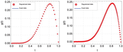
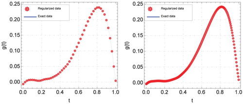
Figure 4. Graphs of exact and regularized data functions for $g(t)$ using new discrete mollification with $\epsilon =0.01$, N = 50 (left panel), and with $\epsilon =0.01$, N = 200 (right panel) for Example 1.

Example 6.2

This example represents an exponential approximation to an instantaneous pulse. The equation for the exact data function is $g(t)=e^{-80(t-0.5{)}^2},0\le t\le 1.$

Example 6.3

This example which is taken to be the same as tested in [18,26,27], concerns a problem with a nonlinear moving interface. In this example, we take $\alpha =1$, $g_2(t)=\sqrt{3-2t}$, $\phi (x)=2x-(x^2/2)-(1/2)$ and the moving interface is given by $s(t)=2-\sqrt{3-2t}.$

The exact solution pair is $\begin{array}{rl}u(x,t)& =2x-\frac{x^2}{2}-t-\frac{1}{2},\\ q(t)& =-t-\frac{1}{2}\end{array}$ and $p(t)=2.$ To assess the accuracy of numerical procedure, we first add random noise $1\mathrm{\%}$ and $5\mathrm{\%}$ to the initial condition (2(2) $u(x,0)=\phi (x),x\in [0,s(0)],s(0)>0,$(2) ) and the Neumann boundary condition (4(4) $\begin{array}{rl}{u}_x(s(t),t)& =g_2(t),t\in [0,T]\end{array}$(4) ), then we employ the new technique of discrete mollification along with the space marching algorithm presented in Section 4 for this test problem. Figures 6–9 illustrate exact and approximate solutions and absolute error for $q(t)$ and $p(t)$, respectively. From these figures, we conclude that at fixed mesh points, the absolute error of numerical results increases by increasing noise level. The RMS and $L_{\mathrm{\infty }}$ errors for this inverse problem with different values of $M_0$ and N are listed in Table 3 with two noise levels $\epsilon =1\mathrm{\%}$ and $5\mathrm{\%}$. This Table shows that at a fixed noise level ϵ, as the number of mesh points increases, the accuracy of the algorithm will improve. Finally, Figure 10 illustrates the graph of the absolute error for $u(x,t)$. This figure demonstrates the effectiveness of the method presented in this paper. We can compare our numerical results with the results of [18,26,27]. However, results of [18,26] for $p(t)$ demonstrate an oscillatory and unstable behaviour (see Figure 12 of [18] and Figures 15 and 17 of [26]) while Figures 8 and 9 show that our method is free of such unstable oscillations. Obviously, comparing Figures 6, 7 and 10 with Figures 6, 7 and 9 of [27] shows that our method perform better, especially for high noise levels. We note that in Examples 3-4, we added the random noise levels to the initial and boundary conditions while in [18,26,27] the noise levels only being applied to the boundary input data. However, our results were even betteer than these Refs.

Figure 5. Graphs of noisy data function $g(t)$ (left panel) and exact and regularized data functions (right panel) using new discrete mollification with $\epsilon =0.1$, N = 128 for Example 2.

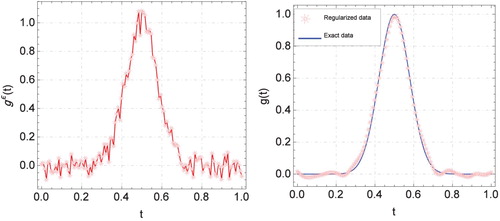
Figure 6. Graphs of exact and computed solutions for $q(t)$ with $\epsilon =1\mathrm{\%}$, $M_0=200$, N = 200 (left panel) and absolute error for $q(t)$ with $\epsilon =1\mathrm{\%}$, $M_0=200$, N = 200 (right panel) for Example 3.

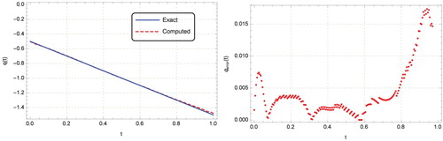
Figure 7. Graphs of exact and computed solutions for $q(t)$ with $\epsilon =5\mathrm{\%}$, $M_0=200$, N = 200 (left panel) and absolute error for $q(t)$ with $\epsilon =0.05$, $M_0=200$, N = 200 (right panel) for Example 3.

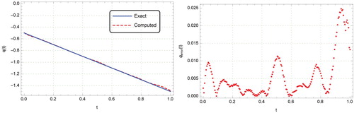
Figure 8. Graphs of exact and computed solutions for $p(t)$ with $\epsilon =1\mathrm{\%}$, $M_0=300$, N = 300 (left panel) and absolute error for $p(t)$ with $\epsilon =1\mathrm{\%}$, $M_0=350$, N = 350 (right panel) for Example 3.

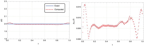
Figure 9. Graphs of exact and computed solutions for $p(t)$ with $\epsilon =5\mathrm{\%}$, $M_0=300$, N = 300 (left panel) and absolute error for $p(t)$ with $\epsilon =5\mathrm{\%}$, $M_0=350$, N = 350 (right panel) for Example 3.

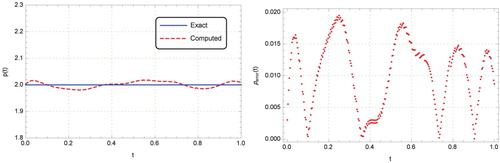
Figure 10. Graph of absolute error for $u(x,t)$ with $\epsilon =5\mathrm{\%}$, $M_0=250$, N = 250 for Example 3.

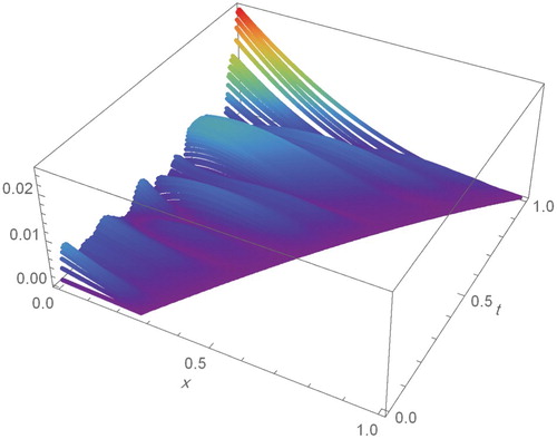
Table 3. RMS and $L_{\mathrm{\infty }}$ for Example 3.

ϵ	$M_0$	N	RMS for $q(t)$	RMS for $p(t)$	$L_{\mathrm{\infty }}$ for $u(x,t)$
$1\mathrm{\%}$	100	100	0.0141423	0.02565570	0.0293676
$5\mathrm{\%}$	100	100	0.0162337	0.02684790	0.0545190
$1\mathrm{\%}$	400	400	0.0058772	0.00824457	0.0117544
$5\mathrm{\%}$	400	400	0.0061947	0.01092980	0.0144669

Example 6.4

In this example [34], we consider problem (1(1) $u_t(x,t)=\alpha u_{xx}(x,t),(x,t)\in D,$(1) )–(6(6) $u_x(0,t)=p(t),t\in [0,T].$(6) ) with $\alpha =1$, $g_2(t)=-(1/\sqrt{2})$, $s(t)=\sqrt{2}-1+(t/\sqrt{2})$, and $\phi (x)=e^{1-(1/\sqrt{2})-(x/\sqrt{2})}.$

The exact solution of this test problem is $\begin{array}{rl}u(x,t)& =e^{1-(1/\sqrt{2})+(t/2)-(x/\sqrt{2})},\\ q(t)& =e^{1-(1/\sqrt{2})+(t/2)},\end{array}$ and $p(t)=-\frac{1}{\sqrt{2}}{e}^{1-(1/\sqrt{2}+(t/2)}.$ We test the accuracy of the proposed method by solving this problem by the above-mentioned method with several values of $M_0$ and N and different noise levels. Figures 11–14 illustrate exact and approximate solutions and absolute error for $q(t)$ and $p(t)$, respectively. From these Figures, we conclude that at fixed mesh points, the absolute error of numerical results increases with increasing noise level. The RMS and $L_{\mathrm{\infty }}$ errors for this inverse problem with different values of $M_0$ and N are listed in Table 4 with two noise levels $\epsilon =1\mathrm{\%}$ and $5\mathrm{\%}$. This Table shows that at a fixed noise level ϵ, as the number of mesh points increases, the accuracy of the algorithm will improve. Finally, Figure 15 illustrates the graph of the absolute error for $u(x,t)$. This figure demonstrates the effectiveness of the method presented in this paper. Our method also performs better than the unregularized decomposition method employed in [34], which is valid only for exact data.

Figure 11. Graphs of exact and computed solutions for $q(t)$ with $\epsilon =1\mathrm{\%}$, $M_0=200$, N = 200 (left panel) and absolute error for $q(t)$ with $\epsilon =1\mathrm{\%}$, $M_0=200$, N = 200 (right panel) for Example 4.

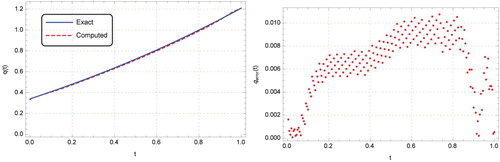
Figure 12. Graphs of exact and computed solutions for $q(t)$ with $\epsilon =5\mathrm{\%}$, $M_0=200$, N = 200 (left panel) and absolute error for $q(t)$ with $\epsilon =5\mathrm{\%}$, $M_0=200$, N = 200 (right panel) for Example 4.

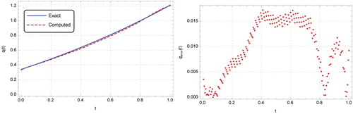
Figure 13. Graphs of exact and computed solutions for $p(t)$ with $\epsilon =1\mathrm{\%}$, $M_0=200$, N = 200 (left panel) and absolute error for $p(t)$ with $\epsilon =1\mathrm{\%}$, $M_0=200$, N = 200 (right panel) for Example 4.

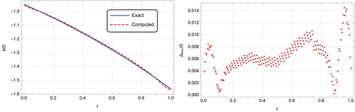
Figure 14. Graphs of exact and computed solutions for $p(t)$ with $\epsilon =5\mathrm{\%}$, $M_0=200$, N = 200 (left panel) and absolute error for $p(t)$ with $\epsilon =5\mathrm{\%}$, $M_0=200$, N = 200 (right panel) for Example 4.

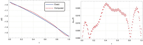
Figure 15. Graph of absolute error for $u(x,t)$ with $\epsilon =5\mathrm{\%}$, $M_0=250$, N = 250 for Example 4.

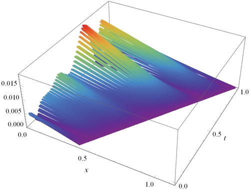
Table 4. RMS and $L_{\mathrm{\infty }}$ for Example 4.

ϵ	$M_0$	N	RMS for $q(t)$	RMS for $p(t)$	$L_{\mathrm{\infty }}$ for $u(x,t)$
$1\mathrm{\%}$	100	100	0.0150765	0.0155459	0.029597
$5\mathrm{\%}$	100	100	0.0160329	0.0176684	0.0303233
$1\mathrm{\%}$	400	400	0.00560614	0.0079557	0.0107032
$5\mathrm{\%}$	400	400	0.0061947	0.0100549	0.0145528

7. Conclusions

In this study, a class of inverse one phase Stefan problem with unknown temperature distribution and heat flux at the boundary x = 0 has been investigated. For solving this problem, a regularization procedure using Bernstein basis polynomials combined with explicit space marching scheme is implemented. As shown in Examples 6.1 and 6.2, by the new technique of discrete mollification, RMS error and especially CPU time are reduced. Moreover, a proof of stability and convergence of the aforementioned algorithm is provided. Finally, the results of this paper have been illustrated by some numerical examples. Numerical examples confirm the efficiency of the proposed method.

References

- Bakal A, Timbers G, Hayakawa K. Solution of the characteristic equation involved in the transient heat conduction for foods approximated by an infinite slab. Can Inst Food Technol. 1970;3:76–77. doi: 10.1016/S0008-3860(70)74275-X
- Conti M. Density change effects on crystal growth from the melt. Phys Rev. 2001;E64:051601.
- Libbrecht KG. The physics of snow crystals. Rep Prog Phys. 2005;68:855–895. doi: 10.1088/0034-4885/68/4/R03
- Lin WS. Steady ablation on the surface of a two-layer composite. Int J Heat Mass Transf. 2005;48:5504–5519. doi: 10.1016/j.ijheatmasstransfer.2005.06.040
- Sharifi N, Bergman TL, Allen MJ, et al. Melting and solidification enhancement using a combined heat pipe foil approach. Int J Heat Mas Tran. 2015;78:930–941. doi: 10.1016/j.ijheatmasstransfer.2014.07.054
- Tayler AB. Mathematical models in applied mechanics. Oxford: ClarendonPress; 2001.
- Namenanee K, McKenzie J, Kosa E, et al. A new approach for catheter ablation of atrial fibrillation: mapping of the electrophysiologic substrate. J Am College Cardiol. 2004;43(11):2044–2053. doi: 10.1016/j.jacc.2003.12.054
- Salva NN, Tarzia DA. Explicit solution for a Stefan problem with variable latent heat and constant heat flux boundary conditions. J Math Anal Appl. 2011;379:240–244. doi: 10.1016/j.jmaa.2010.12.039
- Trueba JL, Voller VR. Analytical and numerical solution of a generalized Stefan problem exhibiting two moving boundaries with application to ocean delta formation. J Math Anal Appl. 2010;366:538–549. doi: 10.1016/j.jmaa.2010.01.008
- Gupta SC. The classical Stefan problem, basic concepts, modelling and analysis. Amsterdam: Elsevier; 2003.
- Crank J. Free and moving boundary problems. Oxford: Clarendon Press; 1984.
- Finlayson BA. The method of weighted residuals and variational principles. New York: Academic Press; 1972.
- Meirmanov AM. The Stefan problem. Berlin: Walter de Gruyter; 1992.
- Ozisik MN. Heat conduction. New York: Wiley; 1980.
- Rubinstein LI. The Stefan problem. Providence: AMS; 1971.
- Goldman NL. Inverse Stefan problem. Dordrecht: Kluwer; 1997.
- Slota D. Direct and inverse one-phase Stefan problem solved by the variational iteration method. Comput Math Appl. 2007;54:113–1146. doi: 10.1016/j.camwa.2006.12.061
- Johansson BT, Lesnic D, Reeve T. A method of fundamental solutions for the one-dimensional inverse Stefan problem. Appl Math Model. 2011;35:4367–4378. doi: 10.1016/j.apm.2011.03.005
- Mitchell SL, Vynnycky M. Finite-difference methods with increased accuracy and correct initialization for one-dimensional Stefan problems. Appl Math Comput. 2009;215:1609–1621.
- Wrobel LC. A boundary element solution to Stefan's problem. Southampton: Computational Mechanics Publications and Berlin: Springer-Verlag; 1983. p. 173–182. (Boundary Elements; V).
- Bollati J, Semitiel J, Tarzia DA. Heat balance integral methods applied to the one-phase Stefan problem with a convective boundary condition at the fixed face. Appl Math Comput. 2018;331:1–19. doi: 10.1016/j.cam.2017.09.008
- Acosta CD, Mejia CE. Stabilization of explicit methods for convection diffusion equations by discrete mollification. Comput Math Appl. 2008;55:368–380. doi: 10.1016/j.camwa.2007.04.019
- Mejia CE, Murio DA. Mollified hyperbolic method for coefficient identification problems. Comput Math Appl. 1993;26(5):1–12. doi: 10.1016/0898-1221(93)90067-6
- Mejia CE, Acosta CD, Saleme KI. Numerical identification of a nonlinear diffusion coefficient by discrete mollification. Comput Math Appl. 2001;62:2187–2199. doi: 10.1016/j.camwa.2011.07.004
- Murio DA. Mollification and space marching, In: Woodbury, K ed. Inverse Engineering Handbook, CRC Press;2002.
- Reddy GMM, Vynnycky M, Cuminato JA. On efficient reconstruction of boundary data with optimal placement of the source points in the MFS: application to inverse Stefan problems. Inverse Probl. Sci. Eng. 2018;26:1249–1279. doi: 10.1080/17415977.2017.1391244
- Reddy GMM, Vynnycky M, Cuminato JA. An efficient adaptive boundary algorithm to reconstruct Neumann boundary data in the MFS for the inverse Stefan problem. J Comput Appl Math. 2019;349:21–40. doi: 10.1016/j.cam.2018.09.004
- Coles C, Murio DA. Identification of parameters in the 2-D IHCP. Comput Math Appl. 2000;40:939–956. doi: 10.1016/S0898-1221(00)85005-1
- Mejia CE, Murio DA. Numerical solution of generalized IHCP by discrete mollification. Comput Math Appl. 1996;32(2):33–50. doi: 10.1016/0898-1221(96)00101-0
- Farin G. Curves and surfaces for computer-Aided geometric design. San Diego: Academic Press; 1997.
- Amiraslani A. Differentiation matrices in polynomial bases. Math Sci. 2016;10:47–53. doi: 10.1007/s40096-016-0177-x
- Farouki RT, Rajan VT. Algorithms for polynomials in Bernstein form. Comput Aided Geom Des. 1988;5:1–26. doi: 10.1016/0167-8396(88)90016-7
- Lorentz GG. Bernstein polynomials. 2nd ed. New York: Chelsea Publishing Co; 1986.
- Grzymkowski R, Slota D. One-phase inverse Stefan problem solved by Adomain decomposition method. Comput Math Appl. 2006;51:33–40. doi: 10.1016/j.camwa.2005.08.028