A meshless computational approach for solving two-dimensional inverse time-fractional diffusion problem with non-local boundary condition

Abstract

This paper is devoted to investigating a two-dimensional inverse anomalous diffusion problem. The missing solely time-dependent Dirichlet boundary condition is recovered by imposing an additional integral measurement over the domain. An efficient computational technique based on a combination of a time integration scheme and local meshless Petrov–Galerkin method is implemented to solve the governing inverse problem. Firstly, an implicit time integration scheme is used to discretize the model in the temporal direction. To fully discretize the model, the primary spatial domain is represented by a set of distributed nodes and data-dependent basis functions are constructed by using the radial point interpolation method. Then, the local meshless Petrov–Galerkin method is used to discretize the problem in the spatial direction. Numerical examples are presented to verify the accuracy and efficiency of the proposed technique. The stability of the method is examined when the input data are contaminated with noise.

Keywords:

• Inverse fractional diffusion problem
• non-local boundary condition
• local meshless petrov–Galerkin method
• radial point interpolation shape functions
• generalized multiquadric radial basis function

2010 Mathematics Subject Classifications:

• 60G22
• 65N21
• 65N30

1. Introduction

Many phenomena and processes in natural sciences, physics and engineering can be mathematically modelled and described as inverse problems. The inverse problem is a problem of determining and identifying inherent characteristics of a physical model, such as identification of material parameters, determination of the shape of domain, identification of initial data, identification of inaccessible boundary conditions and so on. These models are widely appeared in the study of problems related to geophysics [1], quantum scattering theory [2], astronomy [3], medical imaging[4], oceanography [5], optics [6], radar [7], acoustics [8] and etc. Unfortunately, the inverse problems are highly ill-posed in the sense of Hadamard principles [9]. In fact, the existence and uniqueness of solutions or continuity of solutions with respect to small input-data perturbations in these problems cannot be guaranteed. The nonlocal boundary value problems of elliptic [10–12], parabolic [13–26] and hyperbolic [27–31] type equations are an important class of inverse problems which have attracted considerable attention due to their great potential in modelling and describing natural phenomena and physical processes. Undoubtedly, the diffusion process is one of the most important phenomena in natural sciences and physics. The process has been modelled and described using the Fick's second law of diffusion. New scientific findings and experimental results indicate that the classical Fick's second law is not adequate to accurately describe the anomalous diffusion processes in complex media. To describe and interpret this kind of complex diffusion systems, a different approach based on a continuous time random walk model and fractional Fick's law is needed [32, 33]. This indicates that in the anomalous diffusion process, the mean squared displacement of a particle varies nonlinearly with time, $⟨x^2⟩\sim D_{\alpha }{t}^{\alpha }$, when $t\to \mathrm{\infty }$ where $D_{\alpha }$ is the generalized diffusion coefficient. For $\alpha =1$, $0<\alpha <1$ and $\alpha >1$, it characterizes the classical diffusion, subdiffusive and superdiffusive systems, respectively. The anomalous diffusion process can be mathematically modelled by the theory of fractional calculus [34–36].

In this work, the following two-dimensional inverse sub-diffusion problem would be investigated numerically [37, 38]: (1) ${}_0^c{D}_t^{\alpha }u(\mathbf{x},t)=\mathrm{\Delta }u(\mathbf{x},t)+\mathcal{F}(\mathbf{x},t),\mathbf{x}=(x,y)\in \mathrm{\Omega },0\le t\le T$(1) with the following initial and Dirichlet boundary conditions: (2) $\begin{array}{rl}u(\mathbf{x},0)& =u_0\left(\mathbf{x}\right),\mathbf{x}\in \overline{\mathrm{\Omega }},\\ u(\mathbf{x},t)& =f(\mathbf{x},t),\mathbf{x}\in {\mathrm{\Gamma }}_1,0\le t\le T\\ u(\mathbf{x},t)& =g\left(\mathbf{x}\right)h\left(t\right),\mathbf{x}\in {\mathrm{\Gamma }}_2,0\le t\le T,\end{array}$(2) where $u(\mathbf{x},t)$ denotes the density of the diffusing material at location $\mathbf{x}$ and time t, $\mathcal{F}(\mathbf{x},t)$ is source function, Δ is the Laplace operator in two dimensional space, $u_0\left(\mathbf{x}\right)$, $f(\mathbf{x},t)$, $g\left(\mathbf{x}\right)$ are given sufficiently smooth functions, and $h\left(t\right)$ is an unknown function, which describes a time amplitude factor of extra boundary source and should be recovered. $\mathrm{\Omega }\subseteq {\mathbb{R}}^2$ denotes the spatial domain with boundary, $\mathrm{\partial }\mathrm{\Omega }$, which consists of two disjoint parts, $\mathrm{\partial }\mathrm{\Omega }={\mathrm{\Gamma }}_1\cup {\mathrm{\Gamma }}_2$, where ${\mathrm{\Gamma }}_1$ and ${\mathrm{\Gamma }}_2$ denote the accessible and inaccessible parts of the boundary, respectively. In addition, ${}_0^c{D}_t^{\alpha }$ denotes the Caputo fractional derivative of order $\alpha (0<\alpha <1)$ with respect to time that is defined as follows[34]: ${}_0^c{D}_t^{\alpha }u(\mathbf{x},t)=\frac{1}{\mathrm{\Gamma }(1-\alpha )}{\int }_0^t\frac{u_{\xi }(\mathbf{x},\xi )}{(t-\xi {)}^{\alpha }}d\xi ,0<\alpha <1,$ and was used in order to characterize anomalous diffusion phenomena. In dealing with the inverse problem (1(1) ${}_0^c{D}_t^{\alpha }u(\mathbf{x},t)=\mathrm{\Delta }u(\mathbf{x},t)+\mathcal{F}(\mathbf{x},t),\mathbf{x}=(x,y)\in \mathrm{\Omega },0\le t\le T$(1) )–(2(2) $\begin{array}{rl}u(\mathbf{x},0)& =u_0\left(\mathbf{x}\right),\mathbf{x}\in \overline{\mathrm{\Omega }},\\ u(\mathbf{x},t)& =f(\mathbf{x},t),\mathbf{x}\in {\mathrm{\Gamma }}_1,0\le t\le T\\ u(\mathbf{x},t)& =g\left(\mathbf{x}\right)h\left(t\right),\mathbf{x}\in {\mathrm{\Gamma }}_2,0\le t\le T,\end{array}$(2) ), it will attempt to simulate the behaviour of the process and also recover the missing boundary data, $h\left(t\right)$, on the inaccessible boundary ${\mathrm{\Gamma }}_2$. To ensure the well-posedness of the proposed inverse problem, a subsidiary condition is needed. Although, for modelling inverse problems, subsidiary conditions can be imposed locally, by measuring behaviour of the phenomenon in a neighbourhood of some observation sampling points. It is more convenient to use nonlocal conditions as subsidiary conditions. In a typical non-local condition, the behaviour of the process is measured non-locally in the whole domain, $\overline{\mathrm{\Omega }}$ [39, 40]. For example, the boundary conditions may contain integrals of $u(\mathbf{x},t)$ in the whole domain, $\overline{\mathrm{\Omega }}$, or, generally, some non-local operator on $u(\mathbf{x},t)$. In this work, the following additional integral measurement over the whole domain (energy condition) is considered as a subsidiary boundary condition: (3) ${\int }_{\mathrm{\Omega }}u(\mathbf{x},t)d\mathbf{x}=m\left(t\right),0\le t\le T,$(3) where $m\left(t\right)$ is a given sufficiently smooth function. The additional non-local condition (3(3) ${\int }_{\mathrm{\Omega }}u(\mathbf{x},t)d\mathbf{x}=m\left(t\right),0\le t\le T,$(3) ) appears naturally in describing and modeling various physical phenomena which is used as supplementary information to retrieve inaccessible information in the inverse problems. Recently, the existence and uniqueness of the solution for the given time fractional inverse problem are analysed by using the Lax-Milgram Lemma in some suitable Sobolev spaces [37]. Yan and Yang studied the fractional inverse problem (1(1) ${}_0^c{D}_t^{\alpha }u(\mathbf{x},t)=\mathrm{\Delta }u(\mathbf{x},t)+\mathcal{F}(\mathbf{x},t),\mathbf{x}=(x,y)\in \mathrm{\Omega },0\le t\le T$(1) )–(3(3) ${\int }_{\mathrm{\Omega }}u(\mathbf{x},t)d\mathbf{x}=m\left(t\right),0\le t\le T,$(3) ) and implemented an efficient numerical technique based on the method of approximate particular solutions using radial basis functions to solve the model [38]. Our aim of this work is to provide an efficient and stable meshless computational procedure for determining the unknown solution $u(\mathbf{x},t)$ and retrieving the Dirichlet boundary data, $h\left(t\right)$, on the inaccessible boundary.

Meshless methods based on radial basis functions (RBFs) are one of the most effective classes of advanced computational techniques which have been introduced and developed in recent decades [41–43]. They have attracted much attention from researchers because of their excellent performance and high flexibility in dealing with complex physical models with irregular and multi-dimensional spatial domains. Several types of techniques and adaptive algorithms using the meshless procedure have been introduced, developed and used for investigating various kinds of practical physical and engineering problems [44–52]. Also, meshless methods based on the RBFs in both strong and weak forms have been formulated and implemented to solve many types of fractional differential equations [53–59].

In the current work, an effective and stable computational procedure based on a combination of an implicit time integration scheme and the MLPG method [60, 61] is developed and used to approximate the unknown solution $u(\mathbf{x},t)$ and retrieve the missing boundary data $h\left(t\right)$. Also, a stability investigation of the proposed method to deal with the fractional inverse problem (1(1) ${}_0^c{D}_t^{\alpha }u(\mathbf{x},t)=\mathrm{\Delta }u(\mathbf{x},t)+\mathcal{F}(\mathbf{x},t),\mathbf{x}=(x,y)\in \mathrm{\Omega },0\le t\le T$(1) )–(3(3) ${\int }_{\mathrm{\Omega }}u(\mathbf{x},t)d\mathbf{x}=m\left(t\right),0\le t\le T,$(3) ) under strong noise levels and for various fractional orders a is performed. The rest of this paper is organized as follows: In Section 2, an implicit and unconditionally stable time-integration scheme is performed to semi-discretize the fractional model in the time direction. Section 3 is devoted to give some basic concepts of the radial point interpolation method for constructing shape functions in meshless procedure and also a meshless method based on a local weak formulation is presented to fully discretize the model. In Section 4, accuracy, stability and efficiency of the proposed computational technique are verified through some numerical examples. Finally, the paper ends with some concluding remarks in Section 5.

2. Time discretization process

In this section, an implicit and unconditionally stable time-integration scheme is performed to discretize the fractional problem (1(1) ${}_0^c{D}_t^{\alpha }u(\mathbf{x},t)=\mathrm{\Delta }u(\mathbf{x},t)+\mathcal{F}(\mathbf{x},t),\mathbf{x}=(x,y)\in \mathrm{\Omega },0\le t\le T$(1) ) in the time direction. For this purpose, suppose the time interval $[0,T]$ is partitioned uniformly into M sub-intervals $\bigcup _{k=0}^{M-1}[t_k,t_{k+1}]$, where $t_k=k\mathrm{\Delta }t$, $k=0,\dots ,M$ and $\mathrm{\Delta }t=T/M$ is time step size. Then by substituting $t=t_{k+1}$ in the fractional problem (1(1) ${}_0^c{D}_t^{\alpha }u(\mathbf{x},t)=\mathrm{\Delta }u(\mathbf{x},t)+\mathcal{F}(\mathbf{x},t),\mathbf{x}=(x,y)\in \mathrm{\Omega },0\le t\le T$(1) ), we have: (4) ${}_0^c{D}_t^{\alpha }u(\mathbf{x},t_{k+1})=\mathrm{\Delta }u(\mathbf{x},t_{k+1})+\mathcal{F}(\mathbf{x},t_{k+1}),\mathbf{x}\in \mathrm{\Omega },k=0,\dots ,M-1,$(4) where $u(\mathbf{x},t_{k+1})$ denotes the exact value of the function $u(\mathbf{x},t)$ at time step $t_{k+1}$. The time fractional derivative, ${}_0^c{D}_t^{\alpha }u(\mathbf{x},t_{k+1})$, is approximated by using an appropriate time-integration algorithm as follows [62]: (5) $\begin{array}{rl}{}_0^c{D}_t^{\alpha }u(\mathbf{x},t_{k+1})& =\frac{1}{\mathrm{\Gamma }(1-\alpha )}{\int }_0^{t_{k+1}}\frac{u_{\tau }(\mathbf{x},\tau )}{(t_{k+1}-\tau {)}^{\alpha }}d\tau \\ & =\frac{1}{\mathrm{\Gamma }(1-\alpha )}\sum _{s=0}^k\frac{u(\mathbf{x},t_{s+1})-u(\mathbf{x},t_s)}{\mathrm{\Delta }t}{\int }_{t_s}^{t_{s+1}}(t_{k+1}-\tau {)}^{-\alpha }d\tau +R_{k+1}\\ & =\frac{(\mathrm{\Delta }t{)}^{-\alpha }}{\mathrm{\Gamma }(2-\alpha )}\sum _{s=0}^k{w}_s(u^{k-s+1}-u^{k-s})+R_{k+1},\end{array}$(5) where $w_s=(s+1{)}^{1-\alpha }-s^{1-\alpha },s=0,1,\dots ,k$, $u^k=u(\mathbf{x},t_k)$ and $R_{k+1}$ denotes the truncation error of the discretization scheme, which satisfies for any $u(\mathbf{x},t)\in C^2(\mathrm{\Omega }\times [0,\mathrm{\infty }\left)\right)$ in the following relation [62]: $\mid R_{k+1}\mid \le \frac{1}{\mathrm{\Gamma }(2-\alpha )}\left[\frac{1-\alpha }{12}+\frac{2^{2-\alpha }}{2-\alpha }-(1+2^{-\alpha })\right]\underset{0\le t\le t_{k+1}}{max}\left|\frac{{\mathrm{\partial }}^{2}u(\mathbf{x},t)}{\mathrm{\partial }{t}^2}\right|(\mathrm{\Delta }t{)}^{2-\alpha }.$ Now, by rearranging (5(5) $\begin{array}{rl}{}_0^c{D}_t^{\alpha }u(\mathbf{x},t_{k+1})& =\frac{1}{\mathrm{\Gamma }(1-\alpha )}{\int }_0^{t_{k+1}}\frac{u_{\tau }(\mathbf{x},\tau )}{(t_{k+1}-\tau {)}^{\alpha }}d\tau \\ & =\frac{1}{\mathrm{\Gamma }(1-\alpha )}\sum _{s=0}^k\frac{u(\mathbf{x},t_{s+1})-u(\mathbf{x},t_s)}{\mathrm{\Delta }t}{\int }_{t_s}^{t_{s+1}}(t_{k+1}-\tau {)}^{-\alpha }d\tau +R_{k+1}\\ & =\frac{(\mathrm{\Delta }t{)}^{-\alpha }}{\mathrm{\Gamma }(2-\alpha )}\sum _{s=0}^k{w}_s(u^{k-s+1}-u^{k-s})+R_{k+1},\end{array}$(5) ), we obtain: (6) ${}_0^c{D}_t^{\alpha }u(\mathbf{x},t_{k+1})\approx \frac{(\mathrm{\Delta }t{)}^{-\alpha }}{\mathrm{\Gamma }(2-\alpha )}(u^{k+1}+\sum _{s=1}^k(w_{k-s+1}-w_{k-s})u^s-w_k{u}^0).$(6) Substituting the (6(6) ${}_0^c{D}_t^{\alpha }u(\mathbf{x},t_{k+1})\approx \frac{(\mathrm{\Delta }t{)}^{-\alpha }}{\mathrm{\Gamma }(2-\alpha )}(u^{k+1}+\sum _{s=1}^k(w_{k-s+1}-w_{k-s})u^s-w_k{u}^0).$(6) ) in (4(4) ${}_0^c{D}_t^{\alpha }u(\mathbf{x},t_{k+1})=\mathrm{\Delta }u(\mathbf{x},t_{k+1})+\mathcal{F}(\mathbf{x},t_{k+1}),\mathbf{x}\in \mathrm{\Omega },k=0,\dots ,M-1,$(4) ), the following discrete form of the governing fractional model at time step $t_{k+1}$ is obtained: (7) $\frac{(\mathrm{\Delta }t{)}^{-\alpha }}{\mathrm{\Gamma }(2-\alpha )}(u^{k+1}+\sum _{s=1}^k(w_{k-s+1}-w_{k-s})u^s-w_k{u}^0)=\mathrm{\Delta }{u}^{k+1}+{\mathcal{F}}^{k+1},$(7) or equally (8) $u^{k+1}-\lambda \mathrm{\Delta }{u}^{k+1}=(1-w_1)u^k-\sum _{s=1}^{k-1}(w_{k-s+1}-w_{k-s})u^s+w_k{u}^0+\lambda {\mathcal{F}}^{k+1},$(8) where $\lambda =\left(\mathrm{\Delta }t{)}^{\alpha }\mathrm{\Gamma }\right(2-\alpha )$. The stability and convergence of this implicit time discretization scheme for the sub-diffusion models have been analysed in [63].

3. Spatial discretization procedure using the local petrov–Galerkin method

This section is devoted to perform a stable and accurate meshless computational method to fully discretize the semi-descrite model (8(8) $u^{k+1}-\lambda \mathrm{\Delta }{u}^{k+1}=(1-w_1)u^k-\sum _{s=1}^{k-1}(w_{k-s+1}-w_{k-s})u^s+w_k{u}^0+\lambda {\mathcal{F}}^{k+1},$(8) ). For this purpose, the radial point interpolation method [42] is used to construct proper compactly supported shape functions. Then, a meshless approach based on the combination of local Petrov–Galerkin method and collocation technique is implemented for solving the fractional inverse problem with essential boundary and additional nonlocal conditions.

3.1. Local radial point interpolation

Here, the construction methodology of a set of compactly supported data-dependent shape functions based on the local radial point interpolation method is expressed briefly. Considering a set of scattered data points $\{{\mathbf{x}}_{\mathbf{i}}{\}}_{i=1}^N\subset \overline{\mathrm{\Omega }}$ which is represented the spatial domain $\overline{\mathrm{\Omega }}=\mathrm{\Omega }\bigcup \mathrm{\partial }\mathrm{\Omega }$. Local radial point interpolation to approximate a field variable u is defined as [42] (9) $u\left(\mathbf{x}\right)=\sum _{j=1}^{n}R(\parallel \mathbf{x}-{\mathbf{x}}_j{\parallel }_2){\lambda }_j+\sum _{k=1}^m{p}_k\left(\mathbf{x}\right){\eta }_k,\mathbf{x}\in {\mathrm{\Omega }}_l,$(9) where ${\mathrm{\Omega }}_l\subset \overline{\mathrm{\Omega }}$ denotes a neighbourhood of evaluation point $\mathbf{x}$, $R(.)$ is a radial basis function and $p_k(.)$ is the $k-$th monomial basis function. $\parallel \mathbf{x}-{\mathbf{x}}_j{\parallel }_2$ denotes the Euclidean distance between $\mathbf{x}$ and the filed nodes $\{{\mathbf{x}}_j{\}}_{j=1}^n\in {\mathrm{\Omega }}_l$. Furthermore, $\{{\lambda }_j{\}}_{j=1}^n$ and $\{{\eta }_k{\}}_{k=1}^m$ are unknown coefficients that are computed by enforcing the following interpolation and moment conditions, respectively: (10) $\begin{array}{rl}\sum _{j=1}^{n}R(\parallel {\mathbf{x}}_i-{\mathbf{x}}_j{\parallel }_2){\lambda }_j+\sum _{k=1}^m{p}_k\left({\mathbf{x}}_i\right){\eta }_k& =u\left({\mathbf{x}}_i\right),i=1,\dots ,n,\\ \sum _{i=1}^n{p}_k\left({\mathbf{x}}_i\right){\lambda }_i& =0,k=1,2,\dots ,m.\end{array}$(10) The above linear system of algebraic equations can be re-written in the following matrix form (11) $\left(\begin{array}{c}{\mathbf{U}}_a\\ 0\end{array}\right)=\underset{G}{\underbrace{\left(\begin{array}{cc}\mathcal{R}& \mathcal{P}\\ {\mathcal{P}}^T& 0\end{array}\right)}}\underset{\mathrm{\Lambda }}{\underbrace{\left(\begin{array}{c}\lambda \\ \eta \end{array}\right)}}.$(11) where ${\mathbf{U}}_a=\left[u\right({\mathbf{x}}_1),u({\mathbf{x}}_2),\dots ,u({\mathbf{x}}_n){]}^T,\mathrm{\Lambda }=[{\lambda }_1,\dots ,{\lambda }_n,{\eta }_1,\dots ,{\eta }_m],$ and $\mathcal{R}={\left(\begin{array}{cccc}R\left(r_{11}\right)& R\left(r_{12}\right)& \dots & R\left(r_{1n}\right)\\ R\left(r_{21}\right)& R\left(r_{22}\right)& \dots & R\left(r_{2n}\right)\\ ⋮& ⋮& \ddots & ⋮\\ R\left(r_{n1}\right)& R\left(r_{n2}\right)& \dots & R\left(r_{nn}\right)\end{array}\right)}_{n\times n},\mathcal{P}={\left(\begin{array}{ccccc}1& x_1& y_1& \dots & p_m\left({\mathbf{x}}_{\mathbf{1}}\right)\\ 1& x_2& y_2& \dots & p_m\left({\mathbf{x}}_{\mathbf{2}}\right)\\ ⋮& ⋮& ⋮& \ddots & ⋮\\ 1& x_n& y_n& \dots & p_m\left({\mathbf{x}}_{\mathbf{n}}\right)\end{array}\right)}_{n\times m},$ in which $r_{ij}=\parallel {\mathbf{x}}_i-{\mathbf{x}}_j{\parallel }_2$. For any arbitrarily set of distinct scattered points, the resultant moment matrix G is non singular and invertible matrix [42], so the interpolation problem (11(11) $\left(\begin{array}{c}{\mathbf{U}}_a\\ 0\end{array}\right)=\underset{G}{\underbrace{\left(\begin{array}{cc}\mathcal{R}& \mathcal{P}\\ {\mathcal{P}}^T& 0\end{array}\right)}}\underset{\mathrm{\Lambda }}{\underbrace{\left(\begin{array}{c}\lambda \\ \eta \end{array}\right)}}.$(11) ) is well-defined and always the local radial point shape functions can be constructed. Substituting the obtained coefficient vector into (9(9) $u\left(\mathbf{x}\right)=\sum _{j=1}^{n}R(\parallel \mathbf{x}-{\mathbf{x}}_j{\parallel }_2){\lambda }_j+\sum _{k=1}^m{p}_k\left(\mathbf{x}\right){\eta }_k,\mathbf{x}\in {\mathrm{\Omega }}_l,$(9) ), we have: (12) $u\left(\mathbf{x}\right)=[{\mathcal{R}}^T{\mathcal{P}}^T]{\mathbf{G}}^{-1}\left(\begin{array}{c}{\mathbf{U}}_a\\ 0\end{array}\right)=[{\mathrm{\Phi }}^T\left(\mathbf{x}\right){\mathrm{\Psi }}^T\left(\mathbf{x}\right)]\left(\begin{array}{c}{\mathbf{U}}_a\\ 0\end{array}\right)={\mathrm{\Phi }}^T\left(\mathbf{x}\right).{\mathbf{U}}_a,$(12) where ${\mathrm{\Phi }}^T\left(\mathbf{x}\right)=\left[{\varphi }_1\right(\mathbf{x}\left){\varphi }_2\right(\mathbf{x})\dots {\varphi }_n(\mathbf{x}\left)\right]$ forms a set of compactly supported shape functions. The constructed shape functions satisfy partition of unity property and have Kronecker delta function property. Obviously $\mathrm{\forall }\mathbf{x}\in {\mathrm{\Omega }}_l^c=\{\mathbf{x}:\mathbf{x}\notin {\mathrm{\Omega }}_l\},{\varphi }_j\left(\mathbf{x}\right)=0.$ So the field variable $u\left(\mathbf{x}\right)$ at any field node $\mathbf{x}\in \overline{\mathrm{\Omega }}$ can be approximated as (13) $u\left(\mathbf{x}\right)=\sum _{j=1}^N{\varphi }_j\left(\mathbf{x}\right)u_j.$(13) In addition, the derivatives of the sufficiently smooth function $u\left(\mathbf{x}\right)$ in terms of the shape functions can be calculated as (14) $\frac{\mathrm{\partial }u\left(\mathbf{x}\right)}{\mathrm{\partial }x}=\sum _{j=1}^N\frac{\mathrm{\partial }{\varphi }_j\left(\mathbf{x}\right)}{\mathrm{\partial }x}{u}_j,\frac{\mathrm{\partial }u\left(\mathbf{x}\right)}{\mathrm{\partial }y}=\sum _{j=1}^N\frac{\mathrm{\partial }{\varphi }_j\left(\mathbf{x}\right)}{\mathrm{\partial }y}{u}_j.$(14) Here, generalized multiquadric (GMQ) radial basis function is used to construct the shape functions. This type of radial basis functions is defined as $R\left(r\right)=(r^2+c^2{)}^q,c>0,$ the only variable of this function refers to Euclidean distance between the point of interest $\mathbf{x}$ and a field point ${\mathbf{x}}_i$, which in the two dimensional space is $r=\sqrt{(x-x_i{)}^2+(y-y_i{)}^2}$. The generalized multiquadric functions belong to $C^{\mathrm{\infty }}$. For q<0, 0<q<1 and q>1 the GMQ functions are strictly positive definite, strictly conditionally positive definite of order one and strictly conditionally positive definite of order $\lceil q\rceil$, respectively [41]. q = 0.5 and q = −0.5 give the standard multiquadric and inverse multiquadric radial basis functions, respectively. Authors in [64] suggested q = 1.03 for solving some two-dimensional mechanics problems. Also, Xiao et al. proposed q = 1.99 as a suitable value [65]. Recently, Kansa et al. found that the selecting q = 2.5 leads to desirable results [66]. The positive real number c is called the shape parameter. The shape parameter plays an important role in improving the accuracy and stability of the computational methods based on these types of basis functions. Although, several researches have been carried out on finding the best value of c, but finding optimal value for shape parameter is still an open problem. Liu and Gu, in [42] suggested $c={\alpha }_c.d_c$, where ${\alpha }_c$ is a non-negative dimensionless constant and $d_c=S/(\sqrt{N}-1)$ denotes the average of nodal spacing in the two-dimensional domain, where S denotes the area of the domain and N is the number of distributed points.

3.2. The meshless local petrov–Galerkin method

In this section, an efficient computational procedure based on the meshless local Petrov–Galerkin method is performed to fully discretize the time independent model (8(8) $u^{k+1}-\lambda \mathrm{\Delta }{u}^{k+1}=(1-w_1)u^k-\sum _{s=1}^{k-1}(w_{k-s+1}-w_{k-s})u^s+w_k{u}^0+\lambda {\mathcal{F}}^{k+1},$(8) ). For this purpose, both sides of the relation (8(8) $u^{k+1}-\lambda \mathrm{\Delta }{u}^{k+1}=(1-w_1)u^k-\sum _{s=1}^{k-1}(w_{k-s+1}-w_{k-s})u^s+w_k{u}^0+\lambda {\mathcal{F}}^{k+1},$(8) ) are multiplied by a proper test function $v\left(\mathbf{x}\right)$ and integrated over the global domain Ω. So we have $\begin{array}{rl}& {\int }_{\mathrm{\Omega }}{u}^{k+1}\left(\mathbf{x}\right)v\left(\mathbf{x}\right)d\mathrm{\Omega }-\lambda {\int }_{\mathrm{\Omega }}\mathrm{\Delta }{u}^{k+1}\left(\mathbf{x}\right)v\left(\mathbf{x}\right)d\mathrm{\Omega }\\ & =(1-w_1){\int }_{\mathrm{\Omega }}{u}^k\left(\mathbf{x}\right)v\left(\mathbf{x}\right)d\mathrm{\Omega }-\sum _{s=1}^{k-1}(w_{k-s+1}-w_{k-s}){\int }_{\mathrm{\Omega }}{u}^s\left(\mathbf{x}\right)v\left(\mathbf{x}\right)d\mathrm{\Omega }\\ & +w_k{\int }_{\mathrm{\Omega }}{u}^0\left(\mathbf{x}\right)v\left(\mathbf{x}\right)d\mathrm{\Omega }+\lambda {\int }_{\mathrm{\Omega }}\mathcal{F}(\mathbf{x},t_{k+1})v\left(\mathbf{x}\right)d\mathrm{\Omega }.\end{array}$ Using the integration by parts formula and the divergence theorem [67], the following relation is obtained $\begin{array}{rl}& {\int }_{\mathrm{\Omega }}{u}^{k+1}\left(\mathbf{x}\right)v\left(\mathbf{x}\right)d\mathrm{\Omega }+\lambda {\int }_{\mathrm{\Omega }}\mathrm{\nabla }{u}^{k+1}\left(\mathbf{x}\right)\mathrm{\nabla }v\left(\mathbf{x}\right)d\mathrm{\Omega }-\lambda {\int }_{\mathrm{\Gamma }}\frac{\mathrm{\partial }{u}^{k+1}\left(\mathbf{x}\right)}{\mathrm{\partial }\nu }v\left(\mathbf{x}\right)d\mathrm{\Gamma }\\ & =(1-w_1){\int }_{\mathrm{\Omega }}{u}^k\left(\mathbf{x}\right)v\left(\mathbf{x}\right)d\mathrm{\Omega }-\sum _{s=1}^{k-1}(w_{k-s+1}-w_{k-s}){\int }_{\mathrm{\Omega }}{u}^s\left(\mathbf{x}\right)v\left(\mathbf{x}\right)d\mathrm{\Omega }\\ & +w_k{\int }_{\mathrm{\Omega }}{u}^0\left(\mathbf{x}\right)v\left(\mathbf{x}\right)d\mathrm{\Omega }+\lambda {\int }_{\mathrm{\Omega }}\mathcal{F}(\mathbf{x},t_{k+1})v\left(\mathbf{x}\right)d\mathrm{\Omega },\end{array}$ where Γ points to the boundary of Ω and $\overrightarrow{\nu }={\nu }_1\overrightarrow{i}+{\nu }_2\overrightarrow{j}$ is the outward unit normal to the boundary Ω. Moreover, $\mathrm{\partial }u/\mathrm{\partial }\nu =\overrightarrow{\mathrm{\nabla }u}.\overrightarrow{\nu }$. Here, the Heaviside step function $v_i\left(\mathbf{x}\right)=\left\{\begin{array}{l}1\mathbf{x}\in {\mathrm{\Omega }}_i\\ 0\mathbf{x}\notin {\mathrm{\Omega }}_i,\end{array}\right.$ is used as the compactly supported test function [67], where ${\mathrm{\Omega }}_i\subset \mathrm{\Omega }$ is an arbitrary compact sub-domain of the main domain Ω. Whereas the partial derivatives of the Heaviside function are equal to zero, so the following weak form of the governing model is obtained (15) $\begin{array}{rl}& {\int }_{{\mathrm{\Omega }}_i}{u}^{k+1}d\mathrm{\Omega }-\lambda {\int }_{{\mathrm{\Gamma }}_i}\frac{\mathrm{\partial }{u}^{k+1}}{\mathrm{\partial }\nu }d\mathrm{\Gamma }\\ & =(1-w_1){\int }_{{\mathrm{\Omega }}_i}{u}^{k}d\mathrm{\Omega }-\sum _{s=1}^{k-1}(w_{k-s+1}-w_{k-s}){\int }_{{\mathrm{\Omega }}_i}{u}^{s}d\mathrm{\Omega }\\ & +w_k{\int }_{{\mathrm{\Omega }}_i}{u}^{0}d\mathrm{\Omega }+\lambda {\int }_{{\mathrm{\Omega }}_i}{\mathcal{F}}^{k+1}d\mathrm{\Omega },\end{array}$(15) where ${\mathrm{\Gamma }}_i$ denotes the boundary of ${\mathrm{\Omega }}_i$. Now, we consider a set of regularly distributed nodes, $\{{\mathbf{x}}_i{\}}_{i=1}^N$, in the main domain. Suppose that these field nodes are partitioned into three different sets, $\{{\mathbf{x}}_i{\}}_{i=1}^{N_I}$ are located in the interior of Ω, $\{{\mathbf{x}}_i{\}}_{i=N_I+1}^{N_I+N_{{\mathrm{\Gamma }}_1}}$ are placed on ${\mathrm{\Gamma }}_1$, $\{{\mathbf{x}}_i{\}}_{i=N_I+N_{{\mathrm{\Gamma }}_1}+1}^N$ are situated on ${\mathrm{\Gamma }}_2$ and $N=N_I+N_{{\mathrm{\Gamma }}_1}+N_{{\mathrm{\Gamma }}_2}$. The local radial point interpolation method is used to construct the spatial shape functions on these scattered field nodes. Then the unknown function $u^k\left(\mathbf{x}\right)$ at each time level is approximated as (16) $u^k\left(\mathbf{x}\right)=\sum _{j=1}^N{u}_j^{\left(k\right)}{\varphi }_j\left(\mathbf{x}\right),$(16) where at each time level the coefficients $\{u_j^{\left(k\right)}{\}}_{j=1}^N$ are unknown and should be determined. Moreover, for each interior field node ${\mathbf{x}}_i,i=1,\dots ,N_I$ in Ω, we consider local quadrature domain ${\mathrm{\Omega }}_i$ as a neighbourhood of point ${\mathbf{x}}_i$. These sub-domains can have any geometric structure and they cover primary computational domain $\mathrm{\Omega }\subseteq \bigcup _{i=1}^{N_I}{\mathrm{\Omega }}_i$, but for simplicity, they are considered as circles or squares. Now by substituting the representation (16(16) $u^k\left(\mathbf{x}\right)=\sum _{j=1}^N{u}_j^{\left(k\right)}{\varphi }_j\left(\mathbf{x}\right),$(16) ) into the weak form (15(15) $\begin{array}{rl}& {\int }_{{\mathrm{\Omega }}_i}{u}^{k+1}d\mathrm{\Omega }-\lambda {\int }_{{\mathrm{\Gamma }}_i}\frac{\mathrm{\partial }{u}^{k+1}}{\mathrm{\partial }\nu }d\mathrm{\Gamma }\\ & =(1-w_1){\int }_{{\mathrm{\Omega }}_i}{u}^{k}d\mathrm{\Omega }-\sum _{s=1}^{k-1}(w_{k-s+1}-w_{k-s}){\int }_{{\mathrm{\Omega }}_i}{u}^{s}d\mathrm{\Omega }\\ & +w_k{\int }_{{\mathrm{\Omega }}_i}{u}^{0}d\mathrm{\Omega }+\lambda {\int }_{{\mathrm{\Omega }}_i}{\mathcal{F}}^{k+1}d\mathrm{\Omega },\end{array}$(15) ), for all of the interior sub-domains ${\mathrm{\Omega }}_i,i=1,\dots ,N_I$, we have (17) $\begin{array}{rl}& \sum _{j=1}^N\left({\int }_{{\mathrm{\Omega }}_i}{\varphi }_{j}d\mathrm{\Omega }\right)u_j^{(k+1)}-\lambda \sum _{j=1}^N\left({\int }_{{\mathrm{\Gamma }}_i}\frac{\mathrm{\partial }{\varphi }_j}{\mathrm{\partial }\nu }d\mathrm{\Gamma }\right)u_j^{(k+1)}\\ & =(1-w_1)\sum _{j=1}^N\left({\int }_{{\mathrm{\Omega }}_i}{\varphi }_{j}d\mathrm{\Omega }\right)u_j^{\left(k\right)}-\sum _{s=1}^{k-1}\left[\left(w_{k-s+1}-w_{k-s}\right)\sum _{j=1}^N\left({\int }_{{\mathrm{\Omega }}_i}{\varphi }_{j}d\mathrm{\Omega }\right)u_j^{\left(s\right)}\right]\\ & +w_k\sum _{j=1}^N\left({\int }_{{\mathrm{\Omega }}_i}{\varphi }_{j}d\mathrm{\Omega }\right)u_j^{\left(0\right)}+\lambda {\int }_{{\mathrm{\Omega }}_i}{\mathcal{F}}^{k+1}d\mathrm{\Omega },i=1,\dots ,N_I.\end{array}$(17) In our approach, the essential boundary and nonlocal conditions are imposed directly on the proposed field variable. So, for field points $\{{\mathbf{x}}_i{\}}_{i=1}^{N_{{\mathrm{\Gamma }}_1}}$ which are located on the boundary ${\mathrm{\Gamma }}_1$, we have (18) $\sum _{j=1}^N{\varphi }_j\left({\mathbf{x}}_i\right)u_j^{(k+1)}=f({\mathbf{x}}_i,t_{k+1}),i=1,\dots ,N_{{\mathrm{\Gamma }}_1}.$(18) Also, by collocating the boundary conditions at each node $\{{\mathbf{x}}_i{\}}_{i=1}^{N_{{\mathrm{\Gamma }}_2}}$ which are placed on the second part of the boundary, ${\mathrm{\Gamma }}_2$, the following discretized equations, which contain the missing boundary data, are derived (19) $\sum _{j=1}^N{\varphi }_j\left({\mathbf{x}}_i\right)u_j^{(k+1)}-g\left({\mathbf{x}}_i\right)h\left(t_{k+1}\right)=0,i=1,\dots ,N_{{\mathrm{\Gamma }}_2}.$(19) The additional non-classical condition (3(3) ${\int }_{\mathrm{\Omega }}u(\mathbf{x},t)d\mathbf{x}=m\left(t\right),0\le t\le T,$(3) ) is approximated as follows (20) $\sum _{j=1}^N{\varpi }_j{u}_j^{(k+1)}=m\left(t_{k+1}\right),$(20) where ${\varpi }_j$ denotes integral of the ${\varphi }_j\left(\mathbf{x}\right)$ over its support, i.e. ${\varpi }_j={\int }_{{\mathrm{\Omega }}_{l_j}}{\varphi }_j\left(\mathbf{x}\right)d\mathbf{x}$, which can be approximated by any numerical integration rule. By appending algebraic equations (17(17) $\begin{array}{rl}& \sum _{j=1}^N\left({\int }_{{\mathrm{\Omega }}_i}{\varphi }_{j}d\mathrm{\Omega }\right)u_j^{(k+1)}-\lambda \sum _{j=1}^N\left({\int }_{{\mathrm{\Gamma }}_i}\frac{\mathrm{\partial }{\varphi }_j}{\mathrm{\partial }\nu }d\mathrm{\Gamma }\right)u_j^{(k+1)}\\ & =(1-w_1)\sum _{j=1}^N\left({\int }_{{\mathrm{\Omega }}_i}{\varphi }_{j}d\mathrm{\Omega }\right)u_j^{\left(k\right)}-\sum _{s=1}^{k-1}\left[\left(w_{k-s+1}-w_{k-s}\right)\sum _{j=1}^N\left({\int }_{{\mathrm{\Omega }}_i}{\varphi }_{j}d\mathrm{\Omega }\right)u_j^{\left(s\right)}\right]\\ & +w_k\sum _{j=1}^N\left({\int }_{{\mathrm{\Omega }}_i}{\varphi }_{j}d\mathrm{\Omega }\right)u_j^{\left(0\right)}+\lambda {\int }_{{\mathrm{\Omega }}_i}{\mathcal{F}}^{k+1}d\mathrm{\Omega },i=1,\dots ,N_I.\end{array}$(17) )–(20(20) $\sum _{j=1}^N{\varpi }_j{u}_j^{(k+1)}=m\left(t_{k+1}\right),$(20) ), an sparse linear system with $(N+1)$ equations and $(N+1)$ unknown coefficients $\{u_1^{(k+1)},u_2^{(k+1)},\dots ,u_N^{(k+1)},h^{(k+1)}\}$ is resulted. The sparse linear system at $k+1$–th time level is represented as the following matrix form: (21) $\mathbf{A}\left[\begin{array}{c}{\mathbf{U}}^{(k+1)}\\ h^{(k+1)}\end{array}\right]=\sum _{s=1}^k\left(({\omega }_{k-s}-{\omega }_{k-s+1})\mathbf{B}\left[\begin{array}{c}{\mathbf{U}}^{\left(s\right)}\\ h^{\left(s\right)}\end{array}\right]\right)+{\omega }_k\mathbf{B}\left[\begin{array}{c}{\mathbf{U}}^{\left(0\right)}\\ h^{\left(0\right)}\end{array}\right]+{\mathbf{F}}^{(k+1)},$(21) where the matrices $\mathbf{A},\mathbf{B},\mathbf{C}$ and $\mathbf{F}$ are defined as follows $\begin{array}{rl}[{\mathbf{A}}_{ij}{]}_{j=1}^N& =\left\{\begin{array}{ll}{\int }_{{\mathrm{\Omega }}_i}{\varphi }_{j}d{\mathrm{\Omega }}_i-\lambda {\int }_{\mathrm{\partial }{\mathrm{\Omega }}_i}\frac{\mathrm{\partial }{\varphi }_j}{\mathrm{\partial }\nu }d{\mathrm{\Gamma }}_i,& i=1,\dots ,N_I,\\ {\phi }_j\left({\mathbf{x}}_i\right),& i=N_I+1,\dots ,N,\\ {\varpi }_j,& i=N+1,\end{array}\right.\\ [{\mathbf{A}}_{ij}{]}_{j=N+1}& =\left\{\begin{array}{ll}g\left({\mathbf{x}}_i\right),& i=N_I+N_{{\mathrm{\Gamma }}_1}+1,\dots ,N_I+N_{{\mathrm{\Gamma }}_1}+N_{{\mathrm{\Gamma }}_2},\\ 0,& elsewhere,\end{array}\right.\\ {\mathbf{B}}_{ij}& =\left\{\begin{array}{ll}{\int }_{{\mathrm{\Omega }}_i}{\varphi }_{j}d{\mathrm{\Omega }}_i,& i=1,\dots ,N_I,j=1,\dots ,N\\ 0,& elsewhere,\end{array}\right.\end{array}$ and ${\mathbf{F}}_i=\left\{\begin{array}{ll}\lambda {\int }_{{\mathrm{\Omega }}_i}{\mathbf{F}}^{k+1}d{\mathrm{\Omega }}_i,& i=1,\dots ,N_I,\\ f({\mathbf{x}}_i,t_{k+1}),& i=N_I+1,\dots ,N_I+N_{{\mathrm{\Gamma }}_1},\\ 0,& i=N_I+N_{{\mathrm{\Gamma }}_1}+1,\dots ,N,\\ m\left(t_{k+1}\right),& i=N+1.\end{array}\right.$ To start the iterative process, the initial values for $\{u_j^{\left(0\right)}{\}}_{j=0}^N$ and $h\left(0\right)$ are needed. These values are determined by interpolating the initial condition, $u_0\left(\mathbf{x}\right)$ at collocation points, $\{{\mathbf{x}}_i{\}}_{i=1}^N$, and using the following relation $h\left(0\right)=\frac{u_0\left(\mathbf{x}\right)}{g\left(\mathbf{x}\right)},g\left(\mathbf{x}\right)\ne 0.$

4. Numerical results

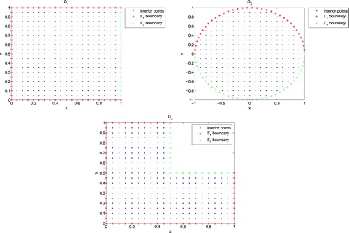
In this section, the efficiency and high performance of the proposed computational procedure to simulate the anomalous diffusion process and determine the missing boundary data are examined. The method is performed to solve three test problems with known exact solutions on three different domains as illustrated in the Figure (1). In the numerical implementation, both regularly and irregularly distributed field nodes in the computational domain are used as the field and evaluation points. The small circles centred at the interior evaluation points with radius $r_q=0.8h$ (h denotes the distance between the nodes in each direction) are selected as the local sub-domains to comply the meshless local weak form, such that, only one evaluation point locates in every local sub-domain, and union of these sub-domains covers all of the global domain. Also, the circles centred at the field points with radius $r_l=4r_q$ are used to construct compactly supported shape functions in the frame of local radial point interpolation method. As mentioned earlier, the GMQ radial basis function with $c={\alpha }_c.d_c$ and q = 2.5 is used to construct the data-dependent shape functions. This type of radial basis functions is conditionally positive definite of order 3, so, to generate the shape functions in the frame of local radial point interpolation method a set of two-dimensional quadratic monomial basis functions .i.e. $P\left(x\right)=\{1,x,y,x^2,xy,y^2\}$ should be used. All of the domain and boundary integrals are evaluated via the $15-$point Gauss quadrature rule. In order to assess the accuracy and validity of the approximate results, three kinds of error measures are used ${\epsilon }_{\mathrm{\infty }}\left(u\right)=\underset{(\mathbf{x},t)\in \mathrm{\Omega }\times [0,T]}{max}|u(\mathbf{x},t)-\tilde{u}(\mathbf{x},t)|,{\epsilon }_{re}\left(u\right)=\frac{\parallel u(\mathbf{x},t)-\tilde{u}(\mathbf{x},t){\parallel }_{\mathrm{\infty }}}{\parallel u(\mathbf{x},t){\parallel }_{\mathrm{\infty }}},$ and ${\epsilon }_{\mathrm{\infty }}\left(h\right)=\underset{0\le k\le M}{max}|h\left(t_k\right)-\tilde{h}\left(t_k\right)|,$ where $u(\mathbf{x},t),h\left(t\right)$ refer to the exact solutions and $\tilde{u}(\mathbf{x},t),\tilde{h}\left(t\right)$ point to the approximate results. Moreover, computational convergence rate of the time discretization scheme is investigated through the following relation: $Rate=\frac{\log \left({\epsilon }_{\mathrm{\infty }}\right(u{)}_{\left(\mathrm{\Delta }{t}_1\right)}/{\epsilon }_{\mathrm{\infty }}\left(u{)}_{\left(\mathrm{\Delta }{t}_2\right)}\right)}{\log \left(\mathrm{\Delta }{t}_1/\mathrm{\Delta }{t}_2\right)}.$ For the sake of completeness, the effects of various factors on the performance of the proposed computational technique are examined, numerically. Especially, the stability of the numerical algorithm to deal with the proposed fractional inverse problem is investigated by imposing random disturbances to all input data $\begin{array}{rl}{\mathbf{F}}_{\sigma }^{(k+1)}& ={\mathbf{F}}^{(k+1)}(1+\mathcal{R}\sigma )\left(inEq\right(21\left)\right)\\ u_0^{\sigma }\left(\mathbf{x}\right)& =u_0\left(\mathbf{x}\right)(1+\mathcal{R}\sigma )\left(inEq\right(2\left)\right),\end{array}$ where $\mathcal{R}$ is a random number between $[-1,1]$ and σ denotes the percentage of imposed noise.

Figure 1. Considered computational domains ${\mathrm{\Omega }}_1$, ${\mathrm{\Omega }}_2$ and ${\mathrm{\Omega }}_3$ and regular distributed nodes in test problems.

4.1. Example 1

In the first example, we consider the fractional inverse problem (1(1) ${}_0^c{D}_t^{\alpha }u(\mathbf{x},t)=\mathrm{\Delta }u(\mathbf{x},t)+\mathcal{F}(\mathbf{x},t),\mathbf{x}=(x,y)\in \mathrm{\Omega },0\le t\le T$(1) )–(3(3) ${\int }_{\mathrm{\Omega }}u(\mathbf{x},t)d\mathbf{x}=m\left(t\right),0\le t\le T,$(3) ) in the three computational domains ${\mathrm{\Omega }}_1,{\mathrm{\Omega }}_2$ and ${\mathrm{\Omega }}_3$, with the analytical solutions [38]: $u(\mathbf{x},t)=t^2{e}^{x+y},h\left(t\right)=t^2,t\in [0,1].$ The initial and boundary data and the source term are extracted from the analytical solutions. The proposed computational technique is performed to solve the model. The numerical results over the considered domains and inaccessible boundaries for $u(x,t)$ and the missing boundary data, $h\left(t\right)$, at various time levels up to t = 1 with $\alpha =0.1$, $\mathrm{\Delta }t=0.005$ and h = 0.05 have been reported in Tables 1–3. Figure 2 shows the spatial convergence with respect to increasing number of field points. From this figure, it is observed that the absolute error decreases when the number of points increases. However, increasing N has no meaningful effect on accuracy, afterward. The obtained approximate solutions along with the absolute errors over the three domains at time level t = 1 with $\mathrm{\Delta }t=0.002$, N = 441 and $\alpha =0.3$ are depicted in Figure 3.

Figure 2. The plots of absolute error functions of Example1 for different number of points N at t = 1 with $\alpha =0.2$ and $\mathrm{\Delta }t=0.01$.

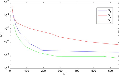
Figure 3. Plot of exact solution and absolute error at T = 1 on ${\mathrm{\Omega }}_1$(a) and plot of absolute error at T = 1 on ${\mathrm{\Omega }}_2$(b) and ${\mathrm{\Omega }}_3$(c) for $\alpha =0.3$ and $\mathrm{\Delta }t=0.002$.

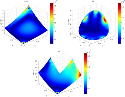
Table 1. Errors estimate results at different time levels up to t = 1 when $\alpha =0.1$ and $\mathrm{\Delta }t=0.005$ for Example 1 on ${\mathrm{\Omega }}_1$.

t	${\epsilon }_{\mathrm{\infty }}\left(u\right)$	${\epsilon }_{re}\left(u\right)$	${\epsilon }_{\mathrm{\infty }}\left(h\right)$
0.1	$2.2708\times {10}^{-6}$	$3.0731\times {10}^{-5}$	$3.3731\times {10}^{-7}$
0.2	$2.2142\times {10}^{-6}$	$7.4916\times {10}^{-6}$	$3.3763\times {10}^{-7}$
0.3	$1.9035\times {10}^{-6}$	$2.8623\times {10}^{-6}$	$3.0627\times {10}^{-7}$
0.4	$1.4241\times {10}^{-6}$	$1.2045\times {10}^{-6}$	$2.5105\times {10}^{-7}$
0.5	$1.2281\times {10}^{-6}$	$6.6482\times {10}^{-7}$	$1.7429\times {10}^{-7}$
0.6	$1.7778\times {10}^{-6}$	$6.6833\times {10}^{-7}$	$7.7038\times {10}^{-8}$
0.7	$2.4276\times {10}^{-6}$	$6.7049\times {10}^{-7}$	$4.0188\times {10}^{-8}$
0.8	$3.1775\times {10}^{-6}$	$6.7191\times {10}^{-7}$	$1.7707\times {10}^{-7}$
0.9	$4.0995\times {10}^{-6}$	$6.8495\times {10}^{-7}$	$3.3340\times {10}^{-7}$
1.0	$5.4135\times {10}^{-6}$	$7.3264\times {10}^{-7}$	$5.0905\times {10}^{-7}$

Table 2. Errors estimate results at different time levels up to t = 1 when $\alpha =0.1$ and $\mathrm{\Delta }t=0.005$ for Example 1 on ${\mathrm{\Omega }}_2$.

t	${\epsilon }_{\mathrm{\infty }}\left(u\right)$	${\epsilon }_{re}\left(u\right)$	${\epsilon }_{\mathrm{\infty }}\left(h\right)$
0.1	$3.9083\times {10}^{-6}$	$9.5052\times {10}^{-5}$	$1.4279\times {10}^{-6}$
0.2	$4.0240\times {10}^{-6}$	$2.4466\times {10}^{-5}$	$1.4577\times {10}^{-6}$
0.3	$7.3324\times {10}^{-6}$	$1.9814\times {10}^{-5}$	$1.3690\times {10}^{-6}$
0.4	$1.2833\times {10}^{-5}$	$1.9507\times {10}^{-5}$	$1.1950\times {10}^{-6}$
0.5	$1.9903\times {10}^{-5}$	$1.9362\times {10}^{-5}$	$9.4581\times {10}^{-7}$
0.6	$2.8543\times {10}^{-5}$	$1.9283\times {10}^{-5}$	$6.2557\times {10}^{-7}$
0.7	$3.8754\times {10}^{-5}$	$1.9235\times {10}^{-5}$	$2.3652\times {10}^{-7}$
0.8	$5.0536\times {10}^{-5}$	$1.9204\times {10}^{-5}$	$2.2006\times {10}^{-7}$
0.9	$6.3890\times {10}^{-5}$	$1.9183\times {10}^{-5}$	$7.4338\times {10}^{-7}$
1.0	$7.8815\times {10}^{-5}$	$1.9168\times {10}^{-5}$	$1.3329\times {10}^{-6}$

Table 3. Errors estimate results at different time levels up to t = 1 when $\alpha =0.1$ and $\mathrm{\Delta }t=0.005$ for Example 1 on ${\mathrm{\Omega }}_3$.

t	${\epsilon }_{\mathrm{\infty }}\left(u\right)$	${\epsilon }_{re}\left(u\right)$	${\epsilon }_{\mathrm{\infty }}\left(h\right)$
0.1	$6.9205\times {10}^{-7}$	$1.5442\times {10}^{-5}$	$1.5981\times {10}^{-7}$
0.2	$6.8592\times {10}^{-7}$	$3.8262\times {10}^{-6}$	$1.5294\times {10}^{-7}$
0.3	$6.1061\times {10}^{-7}$	$1.5138\times {10}^{-6}$	$1.2629\times {10}^{-7}$
0.4	$5.2499\times {10}^{-7}$	$7.3213\times {10}^{-7}$	$8.3586\times {10}^{-8}$
0.5	$8.3171\times {10}^{-7}$	$7.4232\times {10}^{-7}$	$2.5949\times {10}^{-8}$
0.6	$1.2068\times {10}^{-6}$	$7.4798\times {10}^{-7}$	$4.6134\times {10}^{-8}$
0.7	$1.6502\times {10}^{-6}$	$7.5145\times {10}^{-7}$	$1.3241\times {10}^{-7}$
0.8	$2.1619\times {10}^{-6}$	$7.5373\times {10}^{-7}$	$2.3272\times {10}^{-7}$
0.9	$2.7419\times {10}^{-6}$	$7.5532\times {10}^{-7}$	$3.4698\times {10}^{-7}$
1.0	$3.3903\times {10}^{-6}$	$7.5647\times {10}^{-7}$	$4.7512\times {10}^{-7}$

The results reported through the Tables 1–3 and Figure 3 demonstrate the accuracy and high performance of the method to solve the proposed fractional inverse problem. The absolute errors ${\epsilon }_{\mathrm{\infty }}\left(u\right)$ along with computational temporal convergence rates computed using various time step sizes and for some values of fractional order α are presented in Table 4. The results demonstrate that the computational time convergence rate of the method with respect to time discretization is of order $O\left(\mathrm{\Delta }{t}^{2-\alpha }\right)$. As mentioned before, the shape parameter, c, has an important role in the stability and accuracy of the method and choosing a proper value of the shape parameter is very important. Figure 4 illustrates the effect of the shape parameter in the accuracy of the approximate results.

To investigate the stability of the method for dealing with the proposed fractional inverse problem, some random disturbances are imposed on all input data and the effects of these noises on the accuracy of the method are examined numerically. The results for some noise levels are reported in Table 5 which immediately demonstrate the numerical stability of the proposed method.

Figure 4. Absolute error vs shape parameter c with $\alpha =0.1$ and $\mathrm{\Delta }t=0.01$ on ${\mathrm{\Omega }}_1$, ${\mathrm{\Omega }}_2$ and ${\mathrm{\Omega }}_3$ for example1.

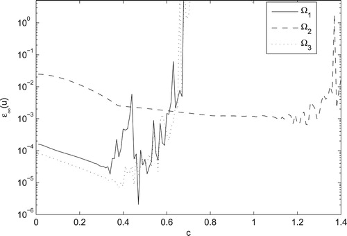
Table 4. Error estimates and convergence rate of Example 1 for different time steps $\mathrm{\Delta }t$.

		${\mathrm{\Omega }}_1$		${\mathrm{\Omega }}_2$		${\mathrm{\Omega }}_3$
α	$\mathrm{\Delta }t$	${\epsilon }_{\mathrm{\infty }}\left(u\right)$	Rate	${\epsilon }_{\mathrm{\infty }}\left(u\right)$	Rate	${\epsilon }_{\mathrm{\infty }}\left(u\right)$	Rate
$\mathbf{0.4}$	$\frac{1}{10}$	$5.1081\times {10}^{-3}$	–	$8.7425\times {10}^{-3}$	–	$1.5427\times {10}^{-3}$	–
	$\frac{1}{20}$	$1.7323\times {10}^{-3}$	1.5601	$2.9707\times {10}^{-3}$	1.5573	$5.2338\times {10}^{-4}$	1.5596
	$\frac{1}{40}$	$5.7905\times {10}^{-4}$	1.5809	$9.9792\times {10}^{-4}$	1.5738	$1.7518\times {10}^{-4}$	1.5790
	$\frac{1}{80}$	$1.8870\times {10}^{-4}$	1.6176	$3.2999\times {10}^{-4}$	1.5965	$5.7335\times {10}^{-5}$	1.6114
	$\frac{1}{160}$	$5.7447\times {10}^{-5}$	1.7158	$1.0537\times {10}^{-4}$	1.6470	$1.7714\times {10}^{-5}$	1.6946
$\mathbf{0.6}$	$\frac{1}{10}$	$1.2635\times {10}^{-2}$	–	$2.1734\times {10}^{-2}$	–	$3.8087\times {10}^{-3}$	–
	$\frac{1}{20}$	$4.8408\times {10}^{-3}$	1.3842	$8.3344\times {10}^{-3}$	1.3828	$1.4592\times {10}^{-3}$	1.3841
	$\frac{1}{40}$	$1.8436\times {10}^{-3}$	1.3927	$3.1794\times {10}^{-3}$	1.3903	$5.5592\times {10}^{-4}$	1.3922
	$\frac{1}{80}$	$6.9699\times {10}^{-4}$	1.4033	$1.2067\times {10}^{-3}$	1.3977	$2.1039\times {10}^{-4}$	1.4018
	$\frac{1}{160}$	$2.5979\times {10}^{-4}$	1.4238	$4.5438\times {10}^{-4}$	1.4091	$7.8647\times {10}^{-5}$	1.4196
$\mathbf{0.8}$	$\frac{1}{10}$	$2.8227\times {10}^{-2}$	–	$4.8858\times {10}^{-2}$	–	$8.4907\times {10}^{-3}$	–
	$\frac{1}{20}$	$1.2322\times {10}^{-2}$	1.1957	$2.1341\times {10}^{-2}$	1.1950	$3.7067\times {10}^{-3}$	1.1958
	$\frac{1}{40}$	$5.3693\times {10}^{-3}$	1.1985	$9.3041\times {10}^{-3}$	1.1977	$1.6152\times {10}^{-3}$	1.1984
	$\frac{1}{80}$	$2.3349\times {10}^{-3}$	1.2014	$4.0506\times {10}^{-3}$	1.1997	$7.0260\times {10}^{-4}$	1.2010
	$\frac{1}{160}$	$1.0122\times {10}^{-3}$	1.2059	$1.7603\times {10}^{-3}$	1.2023	$3.0478\times {10}^{-4}$	1.2049

Table 5. The effect of noise on error estimates when h = .05 and $\mathrm{\Delta }t=.01$ for Example 1.

α	σ	${\mathrm{\Omega }}_1$	${\mathrm{\Omega }}_2$	${\mathrm{\Omega }}_3$
$\mathbf{0.2}$	0	$2.1848\times {10}^{-5}$	$8.1586\times {10}^{-5}$	$6.9823\times {10}^{-6}$
	0.01	$7.4220\times {10}^{-4}$	$4.4852\times {10}^{-4}$	$4.4825\times {10}^{-4}$
	0.1	$7.3923\times {10}^{-3}$	$4.1109\times {10}^{-3}$	$4.4818\times {10}^{-3}$
	1	$7.3894\times {10}^{-2}$	$4.1117\times {10}^{-2}$	$4.4817\times {10}^{-2}$
	5	$3.6946\times {10}^{-1}$	$2.0559\times {10}^{-1}$	$2.2408\times {10}^{-1}$
$\mathbf{0.5}$	0	$2.6256\times {10}^{-4}$	$4.5772\times {10}^{-4}$	$7.9558\times {10}^{-5}$
	0.01	$7.5180\times {10}^{-4}$	$4.7357\times {10}^{-4}$	$4.4829\times {10}^{-4}$
	0.1	$7.4020\times {10}^{-3}$	$4.1100\times {10}^{-3}$	$4.4818\times {10}^{-3}$
	1	$7.3904\times {10}^{-2}$	$4.1116\times {10}^{-2}$	$4.4817\times {10}^{-2}$
	5	$3.6947\times {10}^{-1}$	$2.0559\times {10}^{-1}$	$2.2408\times {10}^{-1}$

4.2. Example 2

As the second benchmark, the performance of the proposed computational technique is examined when applied to the inverse anomalous diffusion problem (1(1) ${}_0^c{D}_t^{\alpha }u(\mathbf{x},t)=\mathrm{\Delta }u(\mathbf{x},t)+\mathcal{F}(\mathbf{x},t),\mathbf{x}=(x,y)\in \mathrm{\Omega },0\le t\le T$(1) )–(3(3) ${\int }_{\mathrm{\Omega }}u(\mathbf{x},t)d\mathbf{x}=m\left(t\right),0\le t\le T,$(3) ) in the spatial domains ${\mathrm{\Omega }}_1,{\mathrm{\Omega }}_2$ and ${\mathrm{\Omega }}_3$ with the following analytical solutions [38]: $u(\mathbf{x},t)=e^{t+x}(1+y),h\left(t\right)=e^t.$ The initial and boundary data and the source term are extracted from the analytical solutions. Tables 6–8 show the numerical results over the considered domains and inaccessible boundaries for $u(x,t)$ and the missing boundary data, $h\left(t\right)$, at various time levels up to t = 1 with $\mathrm{\Delta }t=0.005$, h = 0.05 and $\alpha =0.2$. Figure 5 demonstrates the spatial convergence of the process with respect to the increasing number of nodes.

Table 6. Errors estimate results at different time levels up to t = 1 when $\alpha =0.2$ and $\mathrm{\Delta }t=0.005$ for Example 2 on ${\mathrm{\Omega }}_1$.

t	${\epsilon }_{\mathrm{\infty }}\left(u\right)$	${\epsilon }_{re}\left(u\right)$	${\epsilon }_{\mathrm{\infty }}\left(h\right)$
0.1	$3.5532\times {10}^{-6}$	$5.9138\times {10}^{-7}$	$4.3786\times {10}^{-7}$
0.2	$4.0447\times {10}^{-6}$	$6.0913\times {10}^{-7}$	$5.0812\times {10}^{-7}$
0.3	$4.5316\times {10}^{-6}$	$6.1751\times {10}^{-7}$	$5.7418\times {10}^{-7}$
0.4	$5.0488\times {10}^{-6}$	$6.2250\times {10}^{-7}$	$6.4290\times {10}^{-7}$
0.5	$5.6095\times {10}^{-6}$	$6.2582\times {10}^{-7}$	$7.1663\times {10}^{-7}$
0.6	$6.2227\times {10}^{-6}$	$6.2817\times {10}^{-7}$	$7.9677\times {10}^{-7}$
0.7	$6.8961\times {10}^{-6}$	$6.2990\times {10}^{-7}$	$8.8446\times {10}^{-7}$
0.8	$7.6372\times {10}^{-6}$	$6.3121\times {10}^{-7}$	$9.8074\times {10}^{-7}$
0.9	$8.4540\times {10}^{-6}$	$6.3223\times {10}^{-7}$	$1.0867\times {10}^{-6}$
1.0	$9.3550\times {10}^{-6}$	$6.3303\times {10}^{-7}$	$1.2034\times {10}^{-6}$

Table 7. Errors estimate results at different time levels up to t = 1 when $\alpha =0.2$ and $\mathrm{\Delta }t=0.005$ for Example 2 on ${\mathrm{\Omega }}_2$.

t	${\epsilon }_{\mathrm{\infty }}\left(u\right)$	${\epsilon }_{re}\left(u\right)$	${\epsilon }_{\mathrm{\infty }}\left(h\right)$
0.1	$4.3403\times {10}^{-5}$	$1.1002\times {10}^{-5}$	$5.1428\times {10}^{-7}$
0.2	$4.7908\times {10}^{-5}$	$1.0988\times {10}^{-5}$	$8.1751\times {10}^{-7}$
0.3	$5.2913\times {10}^{-5}$	$1.0981\times {10}^{-5}$	$1.0351\times {10}^{-6}$
0.4	$5.8455\times {10}^{-5}$	$1.0977\times {10}^{-5}$	$1.2316\times {10}^{-6}$
0.5	$6.4586\times {10}^{-5}$	$1.0974\times {10}^{-5}$	$1.4261\times {10}^{-6}$
0.6	$7.1365\times {10}^{-5}$	$1.0972\times {10}^{-5}$	$1.6274\times {10}^{-6}$
0.7	$7.8859\times {10}^{-5}$	$1.0970\times {10}^{-5}$	$1.8406\times {10}^{-6}$
0.8	$8.7142\times {10}^{-5}$	$1.0969\times {10}^{-5}$	$2.0698\times {10}^{-6}$
0.9	$9.6298\times {10}^{-5}$	$1.0968\times {10}^{-5}$	$2.3182\times {10}^{-6}$
1.0	$1.0642\times {10}^{-4}$	$1.0967\times {10}^{-5}$	$2.5890\times {10}^{-6}$

Table 8. Errors estimate results at different time levels up to t = 1 when $\alpha =0.2$ and $\mathrm{\Delta }t=0.005$ for Example 2 on ${\mathrm{\Omega }}_3$.

t	${\epsilon }_{\mathrm{\infty }}\left(u\right)$	${\epsilon }_{re}\left(u\right)$	${\epsilon }_{\mathrm{\infty }}\left(h\right)$
0.1	$3.2206\times {10}^{-6}$	$7.1469\times {10}^{-7}$	$2.1717\times {10}^{-7}$
0.2	$3.5578\times {10}^{-6}$	$7.1438\times {10}^{-7}$	$2.5726\times {10}^{-7}$
0.3	$3.9311\times {10}^{-6}$	$7.1423\times {10}^{-7}$	$2.9333\times {10}^{-7}$
0.4	$4.3439\times {10}^{-6}$	$7.1413\times {10}^{-7}$	$3.3014\times {10}^{-7}$
0.5	$4.8003\times {10}^{-6}$	$7.1406\times {10}^{-7}$	$3.6924\times {10}^{-7}$
0.6	$5.3047\times {10}^{-6}$	$7.1400\times {10}^{-7}$	$4.1151\times {10}^{-7}$
0.7	$5.8623\times {10}^{-6}$	$7.1396\times {10}^{-7}$	$4.5759\times {10}^{-7}$
0.8	$6.4785\times {10}^{-6}$	$7.1393\times {10}^{-7}$	$5.0808\times {10}^{-7}$
0.9	$7.1596\times {10}^{-6}$	$7.1390\times {10}^{-7}$	$5.6354\times {10}^{-7}$
1.0	$7.9123\times {10}^{-6}$	$7.1388\times {10}^{-7}$	$6.2457\times {10}^{-7}$

Moreover, the performance and accuracy of the method to deal with the proposed inverse problem over the three different computational domains are illustrated in Figure 6. To examine the stability and accuracy of the implicit time discretization scheme, the absolute errors along with computational temporal convergence rates with respect to various time step sizes and for some values of fractional order α are presented in Table 9.

The effect of the shape parameter on the accuracy and stability of the method is illustrated in Figure 7. To confirm the performance of the method for investigating the fractional inverse problem, some random disturbances are imposed on all input data and the effects of these noises on the accuracy of the method are examined numerically and reported in Table 10.

Figure 5. Graph of absolute error functions of Example2 for different number of points N at t = 1 with $\alpha =0.1$ and $\mathrm{\Delta }t=0.01$.

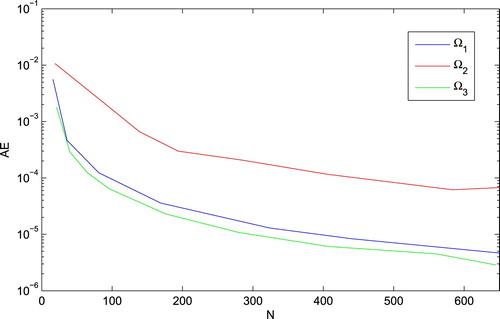
Figure 6. Plot of exact solution and absolute error at T = 1 on ${\mathrm{\Omega }}_1$ (a) and plot of absolute error at T = 1 on ${\mathrm{\Omega }}_2$ (b) and ${\mathrm{\Omega }}_3$ (c) with $\alpha =0.3$ and $\mathrm{\Delta }t=0.002$ for example2.

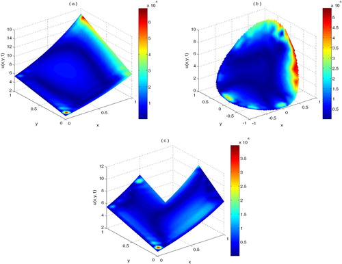
Figure 7. Absolute error vs shape parameter c with $\alpha =0.1$ and $\mathrm{\Delta }t=0.01$ on ${\mathrm{\Omega }}_1$, ${\mathrm{\Omega }}_2$ and ${\mathrm{\Omega }}_3$ for example2.

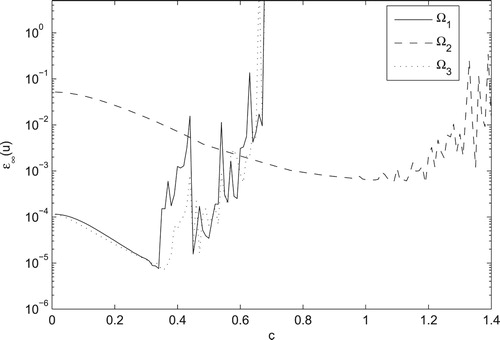
Table 9. Error estimates and convergence rate of Example 2 for different time steps $\mathrm{\Delta }t$.

		${\mathrm{\Omega }}_1$		${\mathrm{\Omega }}_2$		${\mathrm{\Omega }}_3$
α	$\mathrm{\Delta }t$	${\epsilon }_{\mathrm{\infty }}\left(u\right)$	Rate	${\epsilon }_{\mathrm{\infty }}\left(u\right)$	Rate	${\epsilon }_{\mathrm{\infty }}\left(u\right)$	Rate
$\mathbf{0.5}$	$\frac{1}{10}$	$5.4590\times {10}^{-3}$	–	$2.2365\times {10}^{-2}$	–	$2.9622\times {10}^{-3}$	–
	$\frac{1}{20}$	$2.0206\times {10}^{-3}$	1.4339	$8.2621\times {10}^{-3}$	1.4367	$1.0952\times {10}^{-3}$	1.4355
	$\frac{1}{40}$	$7.3711\times {10}^{-4}$	1.4548	$2.9975\times {10}^{-3}$	1.4628	$3.9834\times {10}^{-4}$	1.4591
	$\frac{1}{80}$	$2.6706\times {10}^{-4}$	1.4647	$1.0693\times {10}^{-3}$	1.4871	$1.4313\times {10}^{-4}$	1.4767
	$\frac{1}{160}$	$9.6938\times {10}^{-5}$	1.4620	$3.7136\times {10}^{-4}$	1.5257	$5.0758\times {10}^{-5}$	1.4956
$\mathbf{0.7}$	$\frac{1}{10}$	$1.2948\times {10}^{-2}$	–	$5.3114\times {10}^{-2}$	–	$7.0270\times {10}^{-3}$	–
	$\frac{1}{20}$	$5.4124\times {10}^{-3}$	1.2584	$2.2185\times {10}^{-2}$	1.2595	$2.9363\times {10}^{-3}$	1.2589
	$\frac{1}{40}$	$2.2359\times {10}^{-3}$	1.2754	$9.1492\times {10}^{-3}$	1.2778	$1.2120\times {10}^{-3}$	1.2767
	$\frac{1}{80}$	$9.1804\times {10}^{-4}$	1.2843	$3.7410\times {10}^{-3}$	1.2902	$4.9651\times {10}^{-4}$	1.2874
	$\frac{1}{160}$	$3.7611\times {10}^{-4}$	1.2874	$1.5171\times {10}^{-3}$	1.3021	$2.0231\times {10}^{-4}$	1.2952
$\mathbf{0.9}$	$\frac{1}{10}$	$2.8304\times {10}^{-2}$	–	$1.1629\times {10}^{-1}$	–	$1.5357\times {10}^{-2}$	–
	$\frac{1}{20}$	$1.3462\times {10}^{-2}$	1.0722	$5.5274\times {10}^{-2}$	1.0731	$7.3037\times {10}^{-3}$	1.0722
	$\frac{1}{40}$	$6.3443\times {10}^{-3}$	1.0853	$2.6032\times {10}^{-2}$	1.0863	$3.4414\times {10}^{-3}$	1.0856
	$\frac{1}{80}$	$2.9763\times {10}^{-3}$	1.0920	$1.2197\times {10}^{-2}$	1.0937	$1.6135\times {10}^{-3}$	1.0928
	$\frac{1}{160}$	$1.3933\times {10}^{-3}$	1.0950	$5.6958\times {10}^{-3}$	1.0986	$7.5435\times {10}^{-4}$	1.0969

Table 10. The effect of noise on error estimates when h = .05 and $\mathrm{\Delta }t=.01$ for Example 2.

α	σ	${\mathrm{\Omega }}_1$	${\mathrm{\Omega }}_2$	${\mathrm{\Omega }}_3$
$\mathbf{0.1}$	0	$1.0070\times {10}^{-5}$	$1.0593\times {10}^{-4}$	$1.2004\times {10}^{-5}$
	0.01	$1.4749\times {10}^{-3}$	$9.7060\times {10}^{-4}$	$1.1126\times {10}^{-3}$
	0.1	$1.4777\times {10}^{-2}$	$9.7037\times {10}^{-3}$	$1.1088\times {10}^{-2}$
	1	$1.4778\times {10}^{-1}$	$9.7034\times {10}^{-2}$	$1.1084\times {10}^{-1}$
	5	$7.3890\times {10}^{-1}$	$4.8517\times {10}^{-1}$	$5.5418\times {10}^{-1}$
$\mathbf{0.4}$	0	$9.8641\times {10}^{-5}$	$3.7835\times {10}^{-4}$	$4.9014\times {10}^{-5}$
	0.01	$1.4803\times {10}^{-3}$	$9.6949\times {10}^{-4}$	$1.1123\times {10}^{-3}$
	0.1	$1.4781\times {10}^{-2}$	$9.7026\times {10}^{-3}$	$1.1087\times {10}^{-2}$
	1	$1.4778\times {10}^{-1}$	$9.7033\times {10}^{-2}$	$1.1084\times {10}^{-1}$
	5	$7.3891\times {10}^{-1}$	$4.8517\times {10}^{-1}$	$5.5418\times {10}^{-1}$

4.3. Example 3

As third example, the inverse sub-diffusion problem (1(1) ${}_0^c{D}_t^{\alpha }u(\mathbf{x},t)=\mathrm{\Delta }u(\mathbf{x},t)+\mathcal{F}(\mathbf{x},t),\mathbf{x}=(x,y)\in \mathrm{\Omega },0\le t\le T$(1) )–(3(3) ${\int }_{\mathrm{\Omega }}u(\mathbf{x},t)d\mathbf{x}=m\left(t\right),0\le t\le T,$(3) ) in the spatial domains ${\mathrm{\Omega }}_1,{\mathrm{\Omega }}_2$ and ${\mathrm{\Omega }}_3$ with the following exact solution is considered: $u(\mathbf{x},t)=t^2{e}^{-\left(\right(x-0.5{)}^2+(y-0.5{)}^2)/\text{β}},h\left(t\right)=t^2,t\in [0,1].$ This model is adapted from [68]. The initial and boundary data and the source term are obtained from the exact solutions. In this example, ${\mathrm{\Omega }}_2$, is considered as a circle centred at $(0.5,0.5)$ with radius 0.5. Moreover, in order to investigate the capability of the technique a set of Halton scattered points is used as field points to represent the computational domains ${\mathrm{\Omega }}_1$,${\mathrm{\Omega }}_2$ and ${\mathrm{\Omega }}_3$. The computational domains are illustrated in Figure 8. The suggested numerical technique is employed for solving the current fractional model. Table 11 contains the absolute errors of approximate solutions over the spatial domains and the missing boundary date for various values of fractional order α. Moreover, Figure 9, demonstrates the plots of computed approximate solutions and their absolute errors for N = 1081, $\mathrm{\Delta }t=0.1$, $\alpha =0.1$ and some values of β.

Figure 8. Considered computational domains ${\mathrm{\Omega }}_1$, ${\mathrm{\Omega }}_2$ and ${\mathrm{\Omega }}_3$ and irregular distributed Halton nodes in example3.

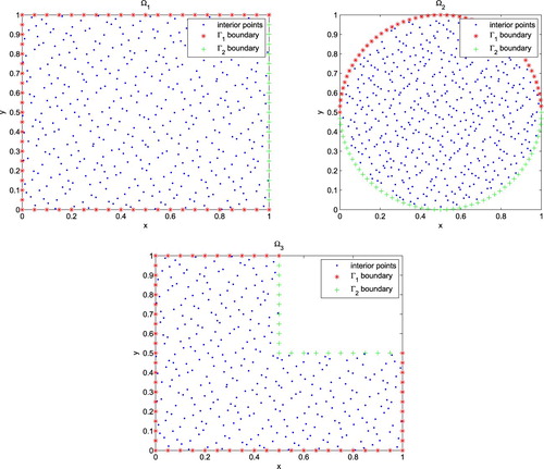
Figure 9. The plot of approximate solutions and their absolute errors for Example 3 on ${\mathrm{\Omega }}_1$ by taking $\alpha =0.1$, N = 1081, $\mathrm{\Delta }t=0.01$ and $\text{β}=0.5$ (a), $\text{β}=0.1$ (b), $\text{β}=0.05$ (c), $\text{β}=0.01$(d) and $\text{β}=0.005$(e).

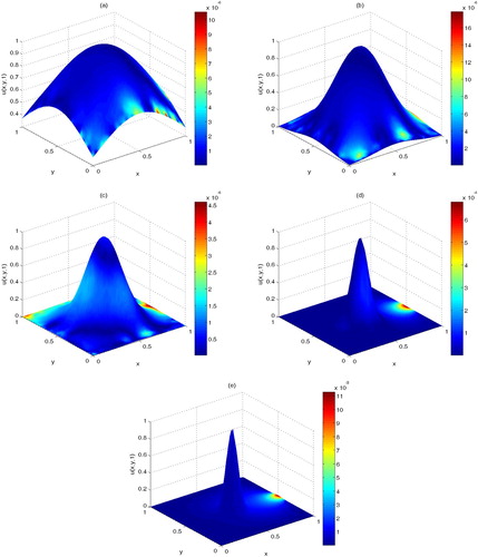
Table 11. Error estimates of Example 3 by letting $\mathrm{\Delta }t=0.01$ and $\text{β}=0.5$ for different values of fractional order α.

	${\mathrm{\Omega }}_1$		${\mathrm{\Omega }}_2$		${\mathrm{\Omega }}_3$
α	${ϵ}_{\mathrm{\infty }}\left(u\right)$	${ϵ}_{\mathrm{\infty }}\left(h\right)$	${ϵ}_{\mathrm{\infty }}\left(u\right)$	${ϵ}_{\mathrm{\infty }}\left(h\right)$	${ϵ}_{\mathrm{\infty }}\left(u\right)$	${ϵ}_{\mathrm{\infty }}\left(h\right)$
$\mathbf{0.2}$	$5.3740\times {10}^{-6}$	$5.0261\times {10}^{-6}$	$1.8004\times {10}^{-4}$	$2.9580\times {10}^{-4}$	$5.1304\times {10}^{-6}$	$9.9655\times {10}^{-7}$
$\mathbf{0.4}$	$2.6329\times {10}^{-5}$	$4.4109\times {10}^{-5}$	$1.7975\times {10}^{-4}$	$2.9533\times {10}^{-4}$	$1.0743\times {10}^{-5}$	$1.0688\times {10}^{-5}$
$\mathbf{0.6}$	$1.0905\times {10}^{-4}$	$1.8060\times {10}^{-4}$	$1.7892\times {10}^{-4}$	$2.9396\times {10}^{-4}$	$4.4420\times {10}^{-5}$	$4.4465\times {10}^{-5}$
$\mathbf{0.8}$	$3.8824\times {10}^{-4}$	$6.4128\times {10}^{-4}$	$1.7629\times {10}^{-4}$	$2.8962\times {10}^{-4}$	$1.5813\times {10}^{-4}$	$1.5822\times {10}^{-4}$

5. Conclusions

In this paper, a two-dimensional inverse anomalous diffusion problem in an arbitrary plane domain has been investigated. An efficient computational technique was performed to simulate the process and retrieve the Dirichlet data on the inaccessible boundary. Firstly, an implicit time stepping procedure was used to discretize the model in the time direction. To fully discretize the model, a local weak form meshless technique was used. In our implementation, the radial point interpolation method was used to construct proper compactly supported spatial shape functions. The accuracy and performance of the proposed method were examined through three benchmarks over three different regular and irregular domains. Numerical findings confirmed the efficiency and accuracy of the presented method to deal with inverse anomalous diffusion problems for retrieving quite accurate missing boundary data. The overall stability of the proposed flexible technique was verified numerically by imposing some random disturbances to input data.

Acknowledgments

The authors would like to thank the referees for providing us with useful and constructive comments and suggestions which improved the quality of the paper.

Disclosure statement

No potential conflict of interest was reported by the author(s).

References

- Backus G, Gilbert F. Uniqueness in the inversion of inaccurate gross earth data. Phil Trans R Soc Lond A. 1970;266(1173):123–192.
- Chadan K, Sabatier PC. Inverse problems in quantum scattering theory. Berlin: Springer Science and Business Media; 2012.
- Craig IJD, Brown JC Inverse problems in astronomy: a guide to inversion strategies for remotely sensed data. Research supported by SERC. Boston (MA): Adam Hilger, Ltd.; 1986, 159 p.
- Arridge SR. Optical tomography in medical imaging. Inverse Probl. 1999;15(2):R41.
- Wunsch C. The ocean circulation inverse problem. New York: Cambridge University Press; 1996.
- Baltes HP. Inverse scattering problems in optics. Berlin: Springer-Verlag; 1980; 1982. p. 423 1795.
- Borden B. Mathematical problems in radar inverse scattering. Inverse Probl. 2001;18(1):R1.
- Gintides D. Local uniqueness for the inverse scattering problem in acoustics via the faber-Krahn inequality. Inverse Probl. 2005;21(4):1195.
- Hadamard J. Lectures on cauchy's problem in linear partial differential equations. Vol. 37. New Haven: Yale University Press; 1923.
- Frey C. On non-local boundary value problems for elliptic operators [diss.]. Köln: Universität zu Köln; 2005.
- Ghosh T, Lin Y-H, Xiao J. The calderon problem for variable coefficients nonlocal elliptic operators. Commun Partial Differ Eq. 2017;42(12):1923–1961.
- Bhattacharyya S, Ghosh T, Uhlmann G Inverse problem for fractional-Laplacian with lower order non-local perturbations. arXiv preprint arXiv:1810.03567; 2018.
- Dehghan M. Alternating direction implicit methods for two-dimensional diffusion with a non-local boundary condition. Int J Comput Math. 1999;72(3):349–366.
- Dehghan M, Tatari M. Use of radial basis functions for solving the second-order parabolic equation with nonlocal boundary conditions. Numer Methods Partial Differ Eq. 2008;24(3):924–938.
- Abbasbandy S, Shirzadi A. A meshless method for two-dimensional diffusion equation with an integral condition. Eng Anal Bound Elem. 2010;34(12):1031–1037.
- Abbasbandy S, Shirzadi A. MLPG method for two-dimensional diffusion equation with neumann's and non-classical boundary conditions. Appl Numer Math. 2011;61(2):170–180.
- Roohani Ghehsareh H, Soltanalizadeh B, Abbasbandy S. A matrix formulation to the wave equation with non-local boundary condition. Int J Comput Math. 2011;88(8):1681–1696.
- Soltanalizadeh B. Numerical analysis of the one-dimensional heat equation subject to a boundary integral specification. Opt Commun. 2011;284(8):2109–2112.
- Kazem S, Rad JA. Radial basis functions method for solving of a non-local boundary value problem with neumann's boundary conditions. Appl Math Model. 2012;36(6):2360–2369.
- Shahmorad S, Borhanifar A, Soltanalizadeh B. An approximation method based on matrix formulated algorithm for the heat equation with nonlocal boundary conditions. Comput Methods Appl Math. 2012;12(1):92–107.
- Abbasbandy S, Ghehsareh HR, Alhuthali MS, et al. Comparison of meshless local weak and strong forms based on particular solutions for a non-classical 2-D diffusion model. Eng Anal Bound Elem. 2014;39:121–128.
- Soltanalizadeh B, Ghehsareh HR, Abbasbandy S. A super accurate shifted tau method for numerical computation of the sobolev-type differential equation with nonlocal boundary conditions. Appl Math Comput. 2014;236:683–692.
- Dehghan M. Parameter determination in a partial differential equation from the overspecified data. Math Comput Model. 2005;41(2–3):196–213.
- Dehghan M. A computational study of the one-dimensional parabolic equation subject to nonclassical boundary specifications. Numer Methods Partial Differ Eq. 2006;22(1):220–257.
- Dehghan M. The one-dimensional heat equation subject to a boundary integral specification. Chaos, Solitons Fractals. 2007;32(2):661–675.
- Ta-Tsien L. A class of non-local boundary value problems for partial differential equations and its applications in numerical analysis. J Comput Appl Math. 1989;28:49–62.
- Ashyralyev A, Ozdemir Y. On nonlocal boundary value problems for hyperbolic-parabolic equations. Dordrecht: Springer; 2007. p. 131–140. (Mathematical Methods in Engineering).
- Salkuyeh DK, Roohani Ghehsareh H. Convergence of the variational iteration method for the telegraph equation with integral conditions. Numer Methods Partial Differ Eq. 2011;27(6):1442–1455.
- Abbasbandy S, Roohani Ghehsareh H. A new semi-analytical solution of the telegraph equation with integral condition. Zeitschrift Für Naturforschung A. 2011;66(12):760–768.
- Shivanian E, Jafarabadi A. Numerical solution of two-dimensional inverse force function in the wave equation with nonlocal boundary conditions. Inverse Probl Sci Eng. 2017;25(12):1743–1767.
- Havlin S, Ben-Avraham D. Diffusion in disordered media. Adv Phys. 1987;36(6):695–798.
- Sokolov IM, Klafter J. From diffusion to anomalous diffusion: a century after einstein's brownian motion. Chaos. 2005;15(2):026103.
- Oldham K, Spanier J. The fractional calculus theory and applications of differentiation and integration to arbitrary order. Vol. 111. New York: Elsevier; 1974.
- Podlubny I. Fractional differential equations: an introduction to fractional derivatives, fractional differential equations, to methods of their solution and some of their applications. Vol. 198. Amsterdam: Elsevier; 1998.
- Uchaikin VV. Fractional derivatives for physicists and engineers. Vol. 2. Berlin: Springer; 2013.
- Asl NA, Rostamy D. Identifying an unknown time-dependent boundary source in time-fractional diffusion equation with a non-local boundary condition. J Comput Appl Math. 2019;355:36–50.
- Yan L, Yang F. The method of approximate particular solutions for the time-fractional diffusion equation with a non-local boundary condition. Comput Math Appl. 2015;70(3):254–264.
- Arendt W, Kunkel S, Kunze M. Diffusion with nonlocal boundary conditions. J Funct Anal. 2016;270(7):2483–2507.
- Arendt W, Kunkel S, Kunze M. Diffusion with nonlocal robin boundary conditions. J Math Soc Jpn. 2018;70(4):1523–1556.
- Fasshauer GE. Meshfree approximation methods with MATLAB. Vol. 6. Singapore: World Scientific; 2007.
- Liu G-R, Gu Y-T. An introduction to meshfree methods and their programming. Berlin: Springer Science and Business Media; 2005.
- Chen W, Fu Z-J, Chen C-S. Recent advances in radial basis function collocation methods. Heidelberg: Springer; 2014.
- Kansa EJ. Multiquadrics-A scattered data approximation scheme with applications to computational fluid-dynamics-I surface approximations and partial derivative estimates. Comput Math Appl. 1990;19(8–9):127–145.
- Abbasbandy S, Roohani Ghehsareh H, Hashim I. A meshfree method for the solution of two-dimensional cubic nonlinear schrodinger equation. Eng Anal Bound Elem. 2013;37(6):885–898.
- Shivanian E, Reza Khodabandehlo H. Meshless local radial point interpolation (MLRPI) on the telegraph equation with purely integral conditions. Eur Phys J Plus. 2014;129(11):241.
- Bengt F, Flyer N. A primer on radial basis functions with applications to the geosciences. Philadelphia: SIAM; 2015.
- Esfahani MH, Roohani Ghehsareh H, Kamal Etesami S. The extended method of approximate particular solutions to simulate two-dimensional electromagnetic scattering from arbitrary shaped anisotropic objects. Eng Anal Bound Elem. 2017;82:91–97.
- Shirzadi A. Numerical solutions of 3D cauchy problems of elliptic operators in cylindrical domain using local weak equations and radial basis functions. Int J Comput Math. 2017;94(2):252–262.
- Dehghan M, Abbaszadeh M. Numerical investigation based on direct meshless local petrov galerkin (direct MLPG) method for solving generalized zakharov system in one and two dimensions and generalized gross-Pitaevskii equation. Eng Comput. 2017;33(4):983–996.
- Taleei A, Dehghan M. Direct meshless local petrov-Galerkin method for elliptic interface problems with applications in electrostatic and elastostatic. Comput Methods Appl Mech Eng. 2014;278:479–498.
- Dehghan M, Haghjoo-Saniji M. The local radial point interpolation meshless method for solving maxwell equations. Eng Comput. 2017;33(4):897–918.
- Chen W, Ye L, Sun H. Fractional diffusion equations by the kansa method. Comput Math Appl. 2010;59(5):1614–1620.
- Gu YT, Zhuang P, Liu F. An advanced implicit meshless approach for the non-linear anomalous subdiffusion equation. Comput Model Eng Sci. 2010;56(3):303–334.
- Dehghan M, Abbaszadeh M, Mohebbi A. An implicit RBF meshless approach for solving the time fractional nonlinear sine-Gordon and klein-Gordon equations. Eng Anal Bound Elem. 2015;50:412–434.
- Shivanian E, Jafarabadi A. An improved spectral meshless radial point interpolation for a class of time-dependent fractional integral equations: 2D fractional evolution equation. J Comput Appl Math. 2017;325:18–33.
- Roohani Ghehsareh H, Zaghian A, Mahmood Zabetzadeh S. The use of local radial point interpolation method for solving two-dimensional linear fractional cable equation. Neural Comput Appl. 2018;29(10):745–754.
- Roohani Ghehsareh H, Zaghian A, Raei M. A local weak form meshless method to simulate a variable order time-fractional mobile-immobile transport model. Eng Anal Bound Elem. 2018;90:63–75.
- Roohani Ghehsareh H, Raei M, Zaghian A. Numerical simulation of a modified anomalous diffusion process with nonlinear source term by a local weak form meshless method. Eng Anal Bound Elem. 2019;98:64–76.
- Atluri SN, Zhu T. A new meshless local petrov-Galerkin (MLPG) approach in computational mechanics. Comput Mech. 1998;22(2):117–127.
- Atluri SN, Zhu TL. A new meshless local petrov-Galerkin (MLPG) approach to nonlinear problems in computer modeling and simulation. Comput Model Simul Eng. 1998;3:187–196.
- Sun Z-Z, Wu X. A fully discrete difference scheme for a diffusion-wave system. Appl Numer Math. 2006;56(2):193–209.
- Liu Q, Gu YT, Zhuang P, et al. An implicit RBF meshless approach for time fractional diffusion equations. Comput Mech. 2011;48(1):1–12.
- Wang JG, Liu GR. On the optimal shape parameters of radial basis functions used for 2-D meshless methods. Comput Methods Appl Mech Eng. 2002;191(23–24):2611–2630.
- Xiao JR, McCarthy MA. A local heaviside weighted meshless method for two-dimensional solids using radial basis functions. Comput Mech. 2003;31(3–4):301–315.
- Kansa EJ, Aldredge RC, Ling L. Numerical simulation of two-dimensional combustion using mesh-free methods. Eng Anal Bound Elem. 2009;33(7):940–950.
- Atluri SN, Shen S. The meshless local petrov-Galerkin (MLPG) method: a simple and less-costly alternative to the finite element and boundary element methods. Comput Model Eng Sci. 2002;3(1):11–51.
- Dehghan M, Abbaszadeh M. Element free galerkin approach based on the reproducing kernel particle method for solving 2D fractional tricomi-type equation with robin boundary condition. Comput Math Appl. 2017;73(6):1270–1285.