
 ?Mathematical formulae have been encoded as MathML and are displayed in this HTML version using MathJax in order to improve their display. Uncheck the box to turn MathJax off. This feature requires Javascript. Click on a formula to zoom.
Abstract
In this paper, the bi-Helmholtz equation with Cauchy conditions is nominated in a n-dimensional strip domain. It is shown that this Cauchy problem may be ill-posed in the sense of Hadamard. In order to overcome the ill-posedness, a suitable regularization method has to be applied to the Cauchy problem. Hence, two well-known wavelet and Fourier regularization methods are used for solving this ill-posed problem. Regarding our experiences, wavelet and Fourier regularization methods act similarly, since these methods remove high frequencies in the frequency space which are the reason for ill-posedness. To explore abilities of the wavelet regularization method, stability of the solution with the Meyer wavelet regularization is investigated by obtaining some error bounds. It is demonstrated numerically that Shannon wavelet is an alternative to the Meyer wavelet in the regularization method. It is explored that the Fourier regularization method for solving the bi-Helmholtz equation with the Cauchy conditions is also applicable. Numerical algorithms of the desired regularization methods are proposed in detail based on the fast Fourier transform (FFT). Various numerical examples in two-dimensional strip domain are shown for the validation and verification of the regularization techniques.
1. Introduction
The Helmholtz-type equation with Cauchy conditions has many applications in engineering and applied sciences; for example, the vibration of structures [Citation1], acoustics [Citation2], electromagnetism [Citation3], wave propagation [Citation4], and scattering [Citation5]. Recently, the ill-posed Cauchy problem for the Helmholtz equation was investigated in a strip domain and some mollification regularization methods have been proposed [Citation6,Citation7]. The Helmholtz equation is also employed in the study of the nonlocal differential beam models of micro- and nano-electromechanical systems, carbon nanotubes, and nanomaterials [Citation8]. In this reference, it has been shown that the bi-Helmholtz type operator is more effective than the Helmholtz type for describing wave dispersion of atomic models. Based on development of the bi-Helmholtz in nonlocal strain-gradient elasticity theory, analysis of wave propagation in a porous double-nanobeam system with graded material properties has been performed in some studies [Citation9,Citation10]. An innovative stress-driven nonlocal integral elastic model of the bi-Helmholtz type has been presented for inflected Bernoulli-Euler nanobeams [Citation11]. From the past to today, the bi-Helmholtz equation on a bounded domain has also several applications in engineering and sciences such as in the boundary element method [Citation12] and streamfunction formulations of the Navier-Stokes equations [Citation13].
This paper is concerned with the study of the ill-posedness of the bi-Helmholtz equation with Cauchy conditions. In fact, it can be proven that this problem has a unique solution which does not depend continuously on the given noisy data. The general approach to overcome the ill-posedness of the Helmholtz and bi-Helmholtz equations with Cauchy conditions is to apply a regularization method. Tikhonov and Fourier regularization methods are some proposed standard and classical techniques to regularize such ill-posed problems [Citation14–16]. However, there are some other techniques such as local discontinuous Galerkin, reproducing kernel, meshless, and Robin-Dirichlet algorithms to tackle some ill-posed problems, see e.g. [Citation17–22].
A technical method for regularizing such problems is the wavelet method. It is worth pointing out that many researchers are interested in exploiting some wavelet bases for solving linear/non-linear partial differential equations with boundary/initial-boundary conditions. One improvement of the wavelet method for solving such problems is the adaptive wavelet method, see e.g. [Citation23–27]. Recently, the wavelet regularization method has come to be exploited as a powerful tool to regularize Cauchy type problems [Citation16,Citation28]. The main goal of this paper is to apply wavelet and Fourier regularization techniques to solve the bi-Helmholtz equation with the Cauchy conditions and study the advantages and drawbacks of these techniques in regularizing the considered problem. One of the most important subjects in the regularization methods is to find an appropriate regularization parameter which depends on both the problem and the method. In ill-posed problems, a regularization parameter can be obtained by an a-periori and/or a-posteriori regularization parameter choice rules [Citation29,Citation30]. Due to the complexity of the Meyer wavelet method and the nature of the bi-Helmholtz equation, we proceed to an a-priori choice rule and leave the a-posteriori choice rule to the future works.
The rest of the paper is organized as follows. Section 2 is devoted to representing the bi-Helmholtz equation with the Cauchy conditions and it is shown that this problem may be ill-posed. In Section 3, a wavelet regularization method is applied for solving the ill-posed problem. To establish analytic results, we choose the Meyer wavelet. Also, we apply the Fourier regularization method in this section. In Section 4, numerical algorithms for the wavelet and Fourier regularization methods based on the FFT are proposed. In Section 5, the regularization methods are illustrated. Finally, Section 6 is devoted to a brief conclusion.
2. Solution and ill-posedness of the bi-Helmholtz Cauchy problem
We consider the following homogeneous bi-Helmholtz equation with Cauchy conditions
(1)
(1) where
and
denote Laplace and bi-Laplace operators, respectively, γ and η are positive real numbers, and
for j = 1, 2, 3, 4 are given functions. Applying multi-dimensional Fourier transform to problem (Equation1
(1)
(1) ) with respect to
, namely,
we have
(2)
(2) By setting
the solution of problem (Equation2
(2)
(2) ) can be written as
where
for
depend on
and
.
Remark 2.1
The study of ill-posedness of problem (Equation1(1)
(1) ) for arbitrary
is very complicated. By setting
and
, we verify that (Equation1
(1)
(1) ) is an ill-posed problem.
The bi-Helmholtz equation with Cauchy conditions in the two-dimensional domain , for
, reads as
(3)
(3) Applying the Fourier transform regarding variable
to problem (Equation3
(3)
(3) ), we have
(4)
(4) The solution of problem (Equation4
(4)
(4) ) is
(5)
(5) and consequently problem (Equation3
(3)
(3) ) has the following solution
Remark 2.2
According to (Equation5(5)
(5) ), ill-posedness of the problem is obvious since small perturbations on
can make dramatic change in output results due to multiplying by terms such as
and
, specially for large
.
To show the ill-posedness of problem (Equation3(3)
(3) ), we consider this problem with
. We impose the following particular perturbation on the measured data
(6)
(6) The corresponding solution arisen from the perturbed data is
(7)
(7) For a fixed 0<
<1, one can verify that
(8)
(8) where 0<
<1 is a constant. When
tends to zero, we have
from (Equation6
(6)
(6) ), while for 0<
<1, we have
from (Equation8
(8)
(8) ). This leads to conclude that problem (Equation3
(3)
(3) ) is ill-posed for the particular case. Similarly, it can be shown that problem (Equation3
(3)
(3) ) is also ill-posed for other cases. For instance, we consider problem (Equation3
(3)
(3) ) for
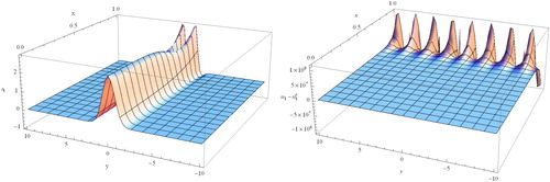
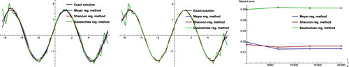
= 1 with
together with the noisy solution stated by (Equation6
(6)
(6) ). The exact solution u and corresponding error
are shown in Figure . The infinity norm of the exact solution on the domain is about 2.8 but the corresponding norm of the noisy solution is more than
while
.
3. Error analysis of wavelet and Fourier regularization methods
The bi-Helmholtz equation with Cauchy conditions has been converted to the frequency space. Since high frequencies cause the ill-posedness, the problem needs to be regularized on the frequency domain. Meyer, Shannon, and Daubechies scaling functions have compact supports in the frequency space. So these scaling functions and their corresponding wavelets can act as low-pass filters to remove high frequencies of the perturbed problem. Regarding to the numerical experiences, we infer that the Meyer and Shannon wavelets can overcome ill-posedness of the problem more effective than Daubechies wavelets. Since the Meyer wavelet and scaling functions are defined in the Fourier domain, therefore we choose the Meyer wavelet in order to find a bound of error and prove the stability of the method. Another reason for selecting the Meyer wavelet is that the Fourier transform of the Meyer wavelet is an analytic function on the frequency domain.
To regularize ill-posed problem (Equation3(3)
(3) ), we decompose its solution to
such that for
is the solution of the following simpler problem
(9)
(9) where
is the Kronecker symbol.
3.1. Meyer wavelet: definitions and properties
According to [Citation31], the Fourier transform of Meyer original scaling and corresponding wavelet functions are given by
where
can be chosen as a
or
function with the property
for all
in
. As an example,
The multiresolution analysis of the Meyer wavelet can be generated by the following nested subspaces
The collection
forms an orthonormal basis for
. In addition, the Fourier transform of wavelet and scaling functions in level
read as
(10)
(10) For all
, the functions in (Equation10
(10)
(10) ) are compactly supported, since
We consider the following projectors
where
and
denotes the inner product in
. Some useful properties of these operators are given as
Bernstein's inequality has a key role in the stability analysis. This inequality is represented in the following lemma [Citation32].
Lemma 3.1
Let be a Meyer multiresolution analysis. For all
it is concluded that
where
is a positive constant and
denotes norm of Sobolev space
defined by
Now, we define the following operators
Proposition 3.2
Let be Meyer multiresolution analysis. For
and any
the following inequalities hold
where
and
is the positive constant in Lemma 3.1.
Proof.
We prove the inequality for the operator . Other cases are similar. According to the definition of the norm
and the solution (Equation5
(5)
(5) ) for
= 1, it is concluded that
Using the Taylor series and Lemma 1 for
, we get
Also, it can be concluded that
Finally, the following result holds
3.2. Regularization method by Meyer wavelet
We focus on the wavelet regularization for problem (Equation9(9)
(9) ) for the case when
= 1. All assumptions, subjects, and proofs in this part are useful and applicable for the remaining cases, i.e. i = 2, 3, 4. Let
be the solution of problem (Equation9
(9)
(9) ) such that the measured data
of
satisfies
for some positive
and non-positive
. This restriction is considered on
, since
for
. We assume that for any
,
, where
is a positive constant.
Proposition 3.3
For a fixed and
in
we have
Proof.
Setting , we define operator
such that
. Thanks to the Parseval formula, one can verify that
Therefore,
Proposition 3.4
For any fixed and
suppose
. For
and
the following inequalities are hold
(11)
(11) where
and
are positive constants.
Proof.
We prove only the first inequality of (Equation11(11)
(11) ). Other inequalities are proved similarly. With considering
and using the result of Proposition 3.2, we show that
To compute the upper bound of
, we define
Then
By setting
the upper-bounds for
is obtained as follows
In the following, we derive upper-bound of
as
So it is concluded that
The first assertion of this proposition appears as follows
Stability of the method is guaranteed by using the following Theorem.
Theorem 3.5
Taking in Proposition 3.4, all of the right hand sides of (Equation11
(11)
(11) ) tend to zero as
since
(12)
(12) and for
(13)
(13) where
for i = 2, 3, 4 are positive constants.
Proof.
Similarly, it is enough to prove the inequality (Equation12(12)
(12) ). According to
, one gets
We have
Substituting these results in the first inequality of (Equation11
(11)
(11) ), we get
3.3. Fourier regularization method
As shown in Section 2, small perturbation on high frequency components is the main reason of ill-posedness. So the idea of the Fourier regularization method is to cut off the high frequencies in the Fourier space. Therefore, the Fourier regularized solution of problem (Equation5(5)
(5) ) is defined as
(14)
(14) where parameter
has to be determined appropriately and
is the characteristic function of interval
. The following theorem proposes a suitable choice of
and presents the corresponding error bounds of the Fourier regularized approximate solution which guarantees the convergence of the method.
Theorem 3.6
For and some
suppose
and
where
is a positive constant. Choosing
the following error estimates hold
(15)
(15) where
is a positive constant.
Proof.
Due to the similarity between the proofs for different , we prove the theorem for
. Using (Equation5
(5)
(5) ) and (Equation14
(14)
(14) ), we have
Exploiting the Parseval relation, we get
4. Numerical algorithms based on FFT
Regarding the effectiveness of the proposed regularization methods in Section 3, the numerical algorithms are given in detail by using the spectral methods based on FFT [Citation33]. Because the solution of problem (Equation3(3)
(3) ) is a periodic function or tends to zero, we solve the problem in the finite domain
, for appropriate a and b. With a fixed
, the interval
is splitted to
subintervals with step length
. In problem (Equation3
(3)
(3) ), input data
are measured by
and the corresponding solutions are denoted by
, respectively. We note that the variable
in the frequency space has to be considered as a vector in the discrete case.
4.1. Discrete Fourier representations for partial derivatives
Discrete Fourier transform is a suitable approach to compute the approximate solution of problem (Equation5(5)
(5) ) (for more detail, see [Citation33]). Without loss of generality, we consider solution
over the domain
. Suppose that
, as
discrete samples of this solution for a fixed
, and
, are approximated by the following discrete fourier representation
(16)
(16) where Fourier coefficients
are obtained as follows
It is worth mentioning that all Fourier coefficients
can be computed from
, or vice versa, in
operations by the FFT algorithm. It is easy to observe that each term
in (Equation16
(16)
(16) ) can be replaced by
for any integer l. Therefore, formula (Equation16
(16)
(16) ) can be reformulated as
The approximate formulae for the first and second derivatives of
with respect to
at
are given as follows
4.2. Wavelet regularization algorithm
In this part, we summarize the wavelet regularization method for the bi-Helmholtz equation with Cauchy conditions in Algorithm 4.1. First, we simulate noisy vectors from given functions
with the error bound ε. Getting
, we discretize functions
to obtain vector
and add a different random real number of interval
to each component of
. The value
can be calculated by the following discrete norm
(17)
(17)
We design the detail of the wavelet regularization algorithm in the following.
4.3. Fourier regularization algorithm
We provide detail of the Fourier regularization method in Algorithm 4.2. In this algorithm, is the parameter of the Fourier regularization method in the discrete form. By the choice of small
, some necessary details of the solution will be missed. For large
, the method will not be able to remove the high frequencies. The suitable approach for determining
is to apply Theorem 3.6.
Remark 4.1
Regarding to in Theorem 3.6, it can be shown that
(18)
(18) where
.
5. Numerical experiments
As observed, applying the Fourier transform to problem (Equation1(1)
(1) ) with perturbed data leads to the ill-posedness. This ill-posedness causes the standard numerical methods not to be able to approximate the exact solution properly. Therefore, application of an appropriate regularization method that matches to the transformed problem is needed. In this section, Fourier and wavelet regularization methods are exploited to the various ill-posed problems that stemmed from Cauchy conditions. To approximate the perturbed given functions in the original problem, we set
such that
In numerical examples, we suppose that
unless we emphasize on some numbers. In Theorem 3.5, we set
, for i = 2, 3, 4. Also, we will consider
for all examples.
Example 5.1
We consider the following Cauchy problems
(19)
(19)
(20)
(20) Algorithm 4.1 is applied to problems (Equation19
(19)
(19) ) and (Equation20
(20)
(20) ) by setting
and
. Results of the applied Meyer wavelet regularization algorithm to problems (Equation19
(19)
(19) ) and (Equation20
(20)
(20) ) for various values of x are reported in Table and Table , respectively. The notation
is used for the wavelet regularization solution with noisy data given in these problems. Thanks to the wavelet regularization method, we conclude that the regularized solution is stabilized when
tends to 1.
Table 1. The corresponding errors of wavelet regularized solution  of problem (Equation19(19) (19) ) for various values of and .
Table 2. The corresponding errors of wavelet regularized solution of problem (Equation20(20) (20) ) for various values of and .
Example 5.2
In this example, we compare the effects of the Meyer, Shannon, and Daubechies wavelets on the following Cauchy problem
(21)
(21) By applying the wavelet regularization Algorithm 4.2, we investigate numerically the effectiveness of these wavelets for problem (Equation21
(21)
(21) ) with the following cases
The results of the Meyer, Shannon, and Daubechies wavelets are reported for Case 1 and Case 2 in Figure and Figure at x = 0.8 and for various values of ε. From Figure and Figure , it is found out that the wavelet regularization method with the Meyer and Shannon wavelets produce better results than the wavelet regularization method with Daubechies wavelet. Although Shannon wavelet is not analytic in the whole of the frequency domain, it can overcome the ill-posedness of Cauchy problems given in this example.
Figure 2. Case 1 of Example 5.2. Plots of the wavelet regularized solutions for at left and middle, respectively. Right: plot of absolute errors versus
at
= 0.8.
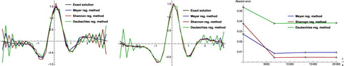
Figure 3. Case 2 of Example 5.2. Plots of wavelet regularized solutions for at left and middle, respectively. Right: plot of absolute errors versus
at
= 0.8.
Example 5.3
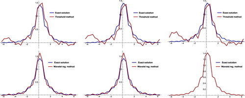
We want to compare the wavelet regularization and wavelet thresholding methods. It is also worth pointing out that the wavelet thresholding method is applied exceedingly to signal denoising and image processing (see e.g. [Citation35–38]) and also the ill-posed problem [Citation34]. In fact, the wavelet regularization method is used without applying any thresholding method. We consider the following problem
(22)
(22) In Algorithm 4.1, we set
. Figure shows that the solution of problem (Equation22
(22)
(22) ), obtained by the wavelet regularization method, tends to exact solution as
decreases to zero while the solution of problem (Equation22
(22)
(22) ), obtained by the thresholding method, does not converge to the exact solution as
.
Figure 4. First row: plots of threshold regularized solutions for Example 5.3 at = 0.5 for
from left to right, respectively, with
= 32. Second row: plots of the corresponding wavelet regularized solutions of first row by using Shannon wavelet.
Example 5.4
In this example, we use the Fourier regularization method and Algorithm 4.2 for solving the following Cauchy problem
(23)
(23) In Algorithm 4.2, we set
. The results of the Fourier regularization method for various values of
and
= 1 are reported in Table . In this table, the notation
is used for the Fourier regularized solution of the Cauchy problem (Equation23
(23)
(23) ). Thanks to the Fourier regularization method, we conclude (see second row of Figure ) that the regularized solution is stabilized when
tends to 1.
Figure 5. First row: plots of exact solutions of problem (Equation23(23)
(23) ) in Example 5.4 with / without noisy data at
= 0.8 for
from left to right, respectively, where
= 128. Second row: plots of exact and Fourier regularized solutions of problem(Equation23
(23)
(23) ) in Example 5.4 with
at
= 0.8 from left to right, respectively.
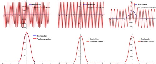
Table 3. The corresponding errors of Fourier regularized solution of problem (Equation23(23) (23) ) in Example 5.4 for s = 1 and various values of x and ε.
6. Conclusion
In this paper, a Cauchy problem of the bi-Helmholtz equation has been studied. It has been shown that this problem may be ill-posed. This situation means that the solution does not depend continuously on the given data. We have figured out that the usage of the regularization technique is mandatory. Among the various regularization methods, wavelet and Fourier regularization methods have been selected. The bi-Helmholtz equation has been transformed to the Fourier domain and explicit expressions of the Fourier transformations of the Meyer wavelet and scaling functions are defined in this domain. Moreover, these functions are analytic in the Fourier domain. Based on these reasons, the wavelet which fits well to our analysis is the Meyer wavelet. By deriving some essential error estimates, we have shown that applying the Meyer wavelet leads to the stability of solutions. Numerical results indicate that Shannon wavelet regularization method is able to regularize the perturbed problem. The Meyer and Shannon wavelets have compact support in the frequency space as well as the Meyer wavelet. So this property of wavelets acts as a low-pass filter for high frequencies which are the source of ill-posedness. There are some restriction when we use wavelets as frequency filters. For instance at finer level of multiresolution and larger regularization parameter , the support of wavelets in frequency space increase exponentially, therefore in practice they can not filter any frequencies. On the other hand, if we choose a small level of multiresolution, wavelets are not able to approximate measured data as much as possible. We suggest a formula for
instead of
to reduce the restrictions. Also, error estimates of the Fourier regularization method show that this method is applicable as well as wavelet regularization methods. In this method, we transform measured data to frequency space and remove high frequencies. The parameter of regularization in Fourier method is the number of components that we choose as high frequencies. From the illustrated examples, wavelet and Fourier regularization methods are two valuable tools to reduce the effect of the ill-posedness as much as possible for solving the bi-Helmholtz equation with Cauchy conditions. We predict that wavelet and Fourier regularization methods can exploit to overcome the ill-posedness of the backward heat conduction problem with time-fractional derivative and a class of non-linear time-dependent partial differential equations. Due to the complexity of the Meyer wavelet method and the nature of the bi-Helmholtz equation, we have obtained the regularization parameter using an a-priori choice rule and we leave an a-posteriori choice rule to the future works.
Acknowledgments
The authors appreciate the reviewers for all valuable comments and suggestions, which helped us to improve the quality of the article.
Disclosure statement
No potential conflict of interest was reported by the author(s).
References
- Beskos DE. Boundary element method in dynamic analysis: part II. Appl Mech Rev. 1997;50:149–197.
- Cen JT, Wong FC. Dual formulation of multiple reciprocity method for the acoustic mode of a cavity with a thin partition. J Sound Vib. 1998;217(1):75–95.
- Hall WS, Mao XQ. Boundary element investigation of irregular frequencies in electromagnetism scattering. Eng Anal Bound Elem. 1995;16:245–252.
- Hong PL, Minh TL, Hoang QP. On a three dimensional Cauchy problem for inhomogeneous Helmholtz equation associated with perturbed wave number. J Comp Appl Math. 2018;335:86–98.
- Marin L, Elliott L, Heggs PJ, et al. Conjugate gradient-boudary element solution to the Cauchy problem for Helmholtz-type equation. Comp Mech. 2003;31:367–377.
- He SQ, Feng XF. A regularization method to solve a Cauchy problem for the two-dimensional modified Helmholtz equation. Mathematics. 2019;360(7):1–13.
- He SQ, Feng XF. A mollification method with Dirichlet kernel to solve Cauchy problem for two-dimensional Helmholtz equation. Int J Wavelets Multiresolut Inf Process. 2019. doi:10.1142/S0219691319500292.
- Koutsoumaris CC, Eptaimeros KG. A research into bi-Helmholtz type of nonlocal elasticity and a direct approach to Eringen's nonlocal integral model in a finite body. Acta Mech. 2018;229:3629–3649.
- Barati MR. Temperature and porosity effects on wave propagation in nanobeams using bi-Helmholtz nonlocal strain-gradient elasticity. Eur Phys J Plus. 2018;133(5):133–170.
- Barati MR, Zenkour A. A general bi-Helmholtz nonlocal strain-gradient elasticity for wave propagation in nanoporous graded double-nanobeam systems on elastic substrate. Compos Struc. 2017;168:885–892.
- Barretta R, Fazelzadeh SA, Feo L, et al. Nonlocal inflected nano-beams: a stress-driven approach of bi-Helmholtz type. Compos Struc. 2018;200:239–245.
- Gaspar C. Multi-level biharmonic and bi-Helmholtz interpolation with application to the boundary element method. Eng Anal Bound Elem. 2000;24:559–573.
- Askham T. A stabilized separation of variables method for the modified biharmonic equation. J Sci Comput. 2019. doi:10.1007/s10915-018-0679-9.
- D'autilia MC, Sgura I, Bozzini B. Parameter identification in ODE models with oscillatory dynamics: a Fourier regularization approach. Inv Prob. 2017;33(12):124009.
- Khieu TT, Vo HH. Recovering the historical distribution for nonlinear space-fractional diffusion equation with temporally dependent thermal conductivity in higher dimensional space. J Comp Appl Math. 2019;345:114–126.
- Li C, Fan Q. Multiplicative noise removal via combining total variation and wavelet frame. Int J Comp Math. 2018;95:2036–2055.
- Berntsson F, Kozlov V, Mpinganzima L. Robin–Dirichlet algorithms for the Cauchy problem for the Helmholtz equation. Inverse Probl Sci Eng. 2017;26(7):1062–1078.
- Caillé L, Delvare F, Marin L, et al. Fading regularization MFS algorithm for the Cauchy problem associated with the two-dimensional Helmholtz equation. Int J Solids Struct. 2017;125:122–133.
- Hua Q, Gu Y, Qu W, et al. A meshless generalized finite difference method for inverse problems associated with three-dimensional inhomogeneous Helmholtz-type equations. Eng Anal Boun Elem. 2017;82:162–171.
- Li M, Hon YC, Chen CS. A meshless method for solving nonhomogeneous Cauchy problems. Eng Anal Boun Elem. 2011;35:499–506.
- Mohammadi M, Mokhtari R, Panahipour H. Solving two parabolic inverse problems with a nonlocal boundary condition in the reproducing kernel space. Appl Comp Math. 2014;13(1):91–106.
- Yeganeh S, Mokhtari R, Hesthaven JS. Space-dependent source determination in a time-fractional diffusion equation using a local discontinuous Galerkin method. BIT Numer Math. 2017;57:685–707.
- Chegini NG, Dahlke S, Friedrich U, et al. Piecewise tensor product wavelet bases by extensions and approximation rates. Math Comp. 2013;82:2157–2190.
- Chegini N, Stevenson R. Adaptive wavelet schemes for parabolic problems: sparse matrices and numerical results. SIAM J Numer Anal. 2011;49(1):182–212.
- Chegini N, Stevenson R. The adaptive tensor product wavelet scheme: sparse matrices and the application to singularly perturbed problems. IMA J Numer Anal. 2012;32(1):75–104.
- Chegini N, Stevenson R. An adaptive wavelet method for semi-linear first-order system least squares. J Comp Meth Appl Math. 2015;15(4):439–463.
- Chegini N, Stevenson R. Adaptive piecewise tensor product wavelets scheme for Laplace-interface problems. J Comput Appl Math. 2018;336:72–97.
- Karimi M, Moradlou F, Hajipour M. On regularization and error estimates for the backward heat conduction problem with time-dependent thermal diffusivity factor. Commun Nonlinear Sci Numer Simul. 2018;63:21–37.
- Kokila J, Nair MT. Fourier truncation method for the non-homogeneous time fractional backward heat conduction problem. Inverse Probl Sci Eng. 2019. doi:10.1080/17415977.2019.1580707.
- Li XX, Li DG. A posteriori regularization parameter choice rule for truncation method for identifying the unknown source of the Poisson equation. Int J Partial Differ Equ. 2013. doi:10.1155/2013/590737.
- Daubechies I. 1992. Ten lectures on wavelets. Society for Industrial and Applied Mathematics 3600. Philadelphia, PA: University City Science Center; 1992.
- Hao DN, Reinhardt HJ, Schneider A. Regularization of a non-characteristic Cauchy problem for a parabolic equation. Inv Prob. 1995;11:1247–1263.
- Kopriva DA. Implementing spectral methods for partial differential equations. Amsterdam: Springer; 2008.
- Karimi M, Rezaee A. Regularization of the Cauchy problem for the Helmholtz equation by using Meyer wavelet. J Comp Appl Math. 2017;320:76–95.
- Akkar HAR, Hadi WAH, Al-Dosari IHM. Implementation of sawtooth wavelet thresholding for noise cancellation in one dimensional signal. Int J Nanoelec Mate. 2019;12(1):67–74.
- Divine OO, Isabona J. Optimum signal denoising based on wavelet shrinkage thresholding techniques: white Gaussian noise and white uniform noise case study. J Sci Eng Res. 2018;5(6):179–186.
- Hedaoo P, Godbole SS. Wavelet thresholding apploach for image denoising. IJNSA. 2011;3:16–21.
- Zhang Y, Ding W, Pan Z. Improved wavelet threshold for image de-noising. Fron Neu Sci. 2019;13(39):1–7.