Lipschitz stability estimate and reconstruction of Lamé parameters in linear elasticity

Abstract

In this paper, we consider the inverse problem of recovering an isotropic elastic tensor from the Neumann-to-Dirichlet map. To this end, we prove a Lipschitz stability estimate for Lamé parameters with certain regularity assumptions. In addition, we assume that the Lamé parameters belong to a known finite subspace with a priori known bounds and that they fulfil a monotonicity property. The proof relies on a monotonicity result combined with the techniques of localized potentials. To numerically solve the inverse problem, we propose a Kohn-Vogelius-type cost functional over a class of admissible parameters subject to two boundary value problems. The reformulation of the minimization problem via the Neumann-to-Dirichlet operator allows us to obtain the optimality conditions by using the Fréchet differentiability of this operator and its inverse. The reconstruction is then performed by means of an iterative algorithm based on a quasi-Newton method. Finally, we give and discuss several numerical examples.

Keywords:

• Lipschitz stability
• monotonicity
• localized potentials
• Lamé parameters

2010 Mathematics Subject Classifications:

• 65J22
• 65M32
• 35R30

1. Introduction

In this paper, we consider the inverse problem of recovering the elastic tensor $\mathbb{C}$ of a linear isotropic elastic body from the Neumann-to-Dirichlet operator $\mathrm{\Lambda }\left(\mathbb{C}\right)$. The main motivations of this problem are non-destructive testing for elastic bodies in order to detect and reconstruct material inclusions (as presented in [1] and the references therein), geophysical (see, e.g. [2]), and medical applications (as considered in [3]), in particular localization of potential tumours via a medical imaging modality called elastography. Elastography is concerned with the reconstruction of the elastic properties in biological tissues and the present article aims at giving access to these features. For a topical review of inverse problems in elasticity and their applications the reader is, e.g. referred to [4].

The paper is split into two parts and gives a twofold perspective on determining Lamé parameters in linear elasticity. Part one is on proving a Lipschitz stability estimate based on the Neumann-to-Dirichlet map for the corresponding tensors ${\mathbb{C}}_1$ and ${\mathbb{C}}_2$, depending on the Lamé parameters $({\lambda }_1,{\mu }_1)$ and $({\lambda }_2,{\mu }_2)$, respectively. The estimate is given under the following a priori assumptions.

1. The Lamé parameters $({\lambda }_j,{\mu }_j)$ for j = 1, 2 belong to a known finite-dimensional subspace, with λ being piecewise continuous and μ being Lipschitz continuous, and with fixed uniform lower and upper bounds.

2. The two pairs of parameters satisfy a monotonicity assumption that $({\lambda }_1,{\mu }_1)$ is, as a pair, either a lower or an upper bound to $({\lambda }_2,{\mu }_2)$.

Part two deals with the reconstruction of the parameters $(\lambda ,\mu )$ based on minimizing a Kohn-Vogelius type functional. Let us stress that this numerical part does not build on the theoretical results presented in Section 3 but rather approaches the problem from a heuristic numerical side to demonstrate that useful numerical reconstructions are indeed possible. It remains a challenging open task how to unite the theoretical and numerical approaches in order to find rigorously justified reconstruction methods that work well in practically relevant settings.

From the theoretical point of view, the inverse problem of recovering $\mathbb{C}$ (or the Lamé moduli $\lambda ,\mu$; cf. (2(2) ${\mathbb{C}}_{ijkl}:=\lambda {\delta }_{ij}{\delta }_{kl}+\mu \left({\delta }_{ik}{\delta }_{jl}+{\delta }_{il}{\delta }_{jk}\right),$(2) )) has been studied by several authors. In the two dimensional case Ikehata [5] proves that the deflection h between $(\lambda +h,\mu +h)$ and $(\lambda ,\mu )$ can be uniquely determined by the first-order approximation of the Dirichlet-to-Neumann operator. Akamatsu et al. [6] give an inversion formula for the normal derivatives at the boundary of the Lamé coefficients $\lambda ,\mu \in C^{\mathrm{\infty }}$ from the Dirichlet-to-Neumann map. At the same time they present stability estimates for the boundary values of $\lambda ,\mu$. Nakamura and Uhlmann [7] established that the Lamé coefficients are uniquely determined from the Dirichlet-to-Neumann operator, assuming that they are sufficiently close to a pair of positive constants. Imanuvilov and Yamamoto [8] proved that the Lamé coefficient λ can be recovered from partial Cauchy data if the coefficient μ is some positive constant. Boundary determination of Lamé coefficients can be found in the work by Lin and Nakamura [9]. In addition, we want to mention a global uniqueness results in 2D by Imanuvilov and Yamamoto [10].

For the three dimensional case, Nakamura and Uhlmann [11,12] and Eskin and Ralston [13] proved uniqueness results for both Lamé coefficients when μ is assumed to be close to a positive constant. The proofs in the above papers rely on the construction of complex geometric optics solutions. For a partial data version, uniqueness for recovering piecewise constant Lamé parameters and a quantitative Lipschitz stability result was proved in [14,15], and some boundary determination results were shown in [9,11,16]. For fully anisotropic $\mathbb{C}$, uniqueness was proved C$\hat{\mathrm{a}}$rstea et al. [17] for a piecewise homogeneous medium. Isakov et al. [18] proved Hölder and Lipschitz stability estimates of determining all coefficients of a dynamical Lamé system with residual stress, including the density Lamé parameters, and the residual stress, by three pairs of observations from the whole boundary or from a part of it. Further on, we want to mention [19], where Hölder stability for non-linear inverse problems is considered.

In this paper, we prove a Lipschitz stability result when the Lamé coefficient λ is piecewise continuous, μ is Lipschitz and a monotonicity assumption holds. In more detail, we assume that the Lamé parameters belong to a known finite subspace with a priori known lower and upper bounds. Our approach relies on the monotonicity of the Neumann-to-Dirichlet operator with respect to the elastic tensor and the techniques of localized potentials [20–26]. For the numerical solution, we reformulate the inverse problem into a minimization problem using a Kohn-Vogelius type cost functional, and use a quasi-Newton method which employs the analytic gradient of the cost function and the approximation of the inverse Hessian is updated by a BFGS (Broyden, Fletcher, Goldfarb, Shanno) scheme [27].

Let us give some more remarks on the relation of this work to previous results. Stability for inverse coefficient problems are derived in general from technically challenging approaches involving quantitative unique continuation estimates and the study of special solutions [11,12,28,29]. Our approach on proving a Lipschitz stability result is relatively simple and easy to extend to other settings, and has already led to new results on uniqueness and Lipschitz stability in electrical impedance tomography (EIT) with finitely many electrodes [30] as well as for the inverse Robin transmission problem [31,32] and on the stability in machine learning reconstruction algorithms [33] under a definiteness assumption. In addition, we want to mention the works [34–38], [39–41] which are concerned with monotonicity-based methods for EIT as well as [42] for monotonicity in inverse medium scattering and [43] for monotonicity methods for the p-Laplace equation.

The paper is organized as follows. In Section 2, we introduce the forward as well as the inverse problem and the Neumann-to-Dirichlet operator. In Section 3, we show a monotonicity result between the Lamé parameters and the Neumann-to-Dirichlet operator and deduce the existence of localized potentials. Then, we prove the Lipschitz stability estimate for a finite-dimensional subset with bounded Lamé parameters and a monotonicity assumption. In Section 4, we present a numerical approach for solving the inverse problem and in Section 5 we show some numerical results.

2. Problem formulation

Let $\mathrm{\Omega }\subset {\mathbb{R}}^d$ $(d\ge 2)$, be a bounded and connected open set, occupied by an isotropic material with linear stress-strain relation. The boundary $\mathrm{\partial }\mathrm{\Omega }$, is assumed to be $C^{1,1}$ and consists of two non-empty disjoint open parts, the fixed ‘Dirichlet-boundary’ ${\mathrm{\Gamma }}_D$ and the ‘Neumann-boundary’ ${\mathrm{\Gamma }}_N$ with $\mathrm{\partial }\mathrm{\Omega }=\overline{{\mathrm{\Gamma }}_N}\cup \overline{{\mathrm{\Gamma }}_D},{\mathrm{\Gamma }}_N\cap {\mathrm{\Gamma }}_D=\mathrm{\varnothing }.$ The choice of mixed boundary conditions is based on the physical treatment of the elasticity problem. The Neumann-to-Dirichlet operator with fixed Dirichlet part is an idealized model for fixing an elastic object in place on one part of the boundary, applying different pressure patterns to the remaining part and measuring the resulting displacements.

We denote a given surface load by $g\in L^2({\mathrm{\Gamma }}_N{)}^d$. Then the displacement vector $u:\overline{\mathrm{\Omega }}\to {\mathbb{R}}^d$ satisfies the following boundary value problem (1) $\begin{array}{rl}-\mathrm{d}\mathrm{i}\mathrm{v}\left(\mathbb{C}\hat{\mathrm{\nabla }}u\right)& =0\mathrm{i}\mathrm{n}\mathrm{\Omega },\\ \left(\mathbb{C}\hat{\mathrm{\nabla }}u\right)\nu & =g\mathrm{o}\mathrm{n}{\mathrm{\Gamma }}_N,\\ u& =0\mathrm{o}\mathrm{n}{\mathrm{\Gamma }}_D,\end{array}$(1) where ν is the outer unit normal vector to $\mathrm{\partial }\mathrm{\Omega }$, which is similar to the boundary value problem considered, e.g. in [44]. The linearized strain tensor $\hat{\mathrm{\nabla }}u$ and the stress tensor $\mathbb{C}\hat{\mathrm{\nabla }}u$ are given by $\hat{\mathrm{\nabla }}u=\frac{1}{2}\left(\mathrm{\nabla }u+(\mathrm{\nabla }u{)}^T\right),\mathbb{C}\hat{\mathrm{\nabla }}u={\left(\sum _{k,l=1}^d{\mathbb{C}}_{ijkl}\frac{\mathrm{\partial }{u}_k}{\mathrm{\partial }{x}_l}\right)}_{1\le i,j\le d},$ where $\mathrm{\nabla }u\left(x\right)=\left(\frac{\mathrm{\partial }}{\mathrm{\partial }{x}_1}u\left(x\right),\dots ,\frac{\mathrm{\partial }}{\mathrm{\partial }{x}_d}u\left(x\right)\right),\mathrm{d}\mathrm{i}\mathrm{v}F\left(x\right)=\left(\begin{array}{c}\sum _{i=1}^d\frac{\mathrm{\partial }}{\mathrm{\partial }{x}_i}{F}_{i1}\left(x\right)\\ ⋮\\ \sum _{i=1}^d\frac{\mathrm{\partial }}{\mathrm{\partial }{x}_i}{F}_{id}\left(x\right)\end{array}\right)$ for $F:\mathrm{\Omega }\mapsto {\mathbb{R}}^{d\times d}$. The isotropic elastic tensor is defined as (2) ${\mathbb{C}}_{ijkl}:=\lambda {\delta }_{ij}{\delta }_{kl}+\mu \left({\delta }_{ik}{\delta }_{jl}+{\delta }_{il}{\delta }_{jk}\right),$(2) where $\lambda ,\mu$ are the Lamé coefficients.

Next, we state a unique continuation principle from [45] (see also [46] for a recent related result):

Theorem 2.1

Weak Unique Continuation Principle

Let Ω be a connected open set in ${\mathbb{R}}^d$ for $d\ge 2$. Let $\mu \left(x\right)\in C^{0,1}\left(\mathrm{\Omega }\right)$ and $\lambda \left(x\right)\in L^{\mathrm{\infty }}\left(\mathrm{\Omega }\right)$ satisfy $\begin{array}{rl}& \mu \left(x\right)\ge {\delta }_0,\lambda \left(x\right)+2\mu \left(x\right)\ge {\delta }_0\mathrm{a}.\mathrm{e}.x\in \mathrm{\Omega },\\ & \parallel \mu {\parallel }_{C^{0,1}\left(\mathrm{\Omega }\right)}+\parallel \lambda {\parallel }_{L^{\mathrm{\infty }}\left(\mathrm{\Omega }\right)}\le M_0,\end{array}$ with positive constants ${\delta }_0,$ $M_0,$ where we define $\parallel f{\parallel }_{C^{0,1}\left(\mathrm{\Omega }\right)}=\parallel f{\parallel }_{L^{\mathrm{\infty }}\left(\mathrm{\Omega }\right)}+\parallel \mathrm{\nabla }f{\parallel }_{L^{\mathrm{\infty }}\left(\mathrm{\Omega }\right)}$. If $u\in H^1(\mathrm{\Omega }{)}^d$ satisfies $\begin{array}{rl}-\mathrm{d}\mathrm{i}\mathrm{v}\left(\mathbb{C}\hat{\mathrm{\nabla }}u\right)& =0in\mathrm{\Omega },\\ u& =0insomeballB\subset \mathrm{\Omega },\end{array}$ then u = 0 in Ω.

Proof.

The reader is referred to Theorem 1.2 from [45].

Corollary 2.2

Unique Continuation Principle for Local Cauchy Data

Let the same assumptions as in Theorem 2.1 hold and let Ω have a $C^{1,1}$ boundary and let Γ be a non-empty open subset of $\mathrm{\partial }\mathrm{\Omega }$. If $u\in H^1(\mathrm{\Omega }{)}^d$ satisfies $\begin{array}{rl}-\mathrm{d}\mathrm{i}\mathrm{v}\left(\mathbb{C}\hat{\mathrm{\nabla }}u\right)& =0\mathrm{i}\mathrm{n}\mathrm{\Omega },\\ \left(\mathbb{C}\hat{\mathrm{\nabla }}u\right)\nu & =0\mathrm{o}\mathrm{n}\mathrm{\Gamma },\\ u& =0\mathrm{o}\mathrm{n}\mathrm{\Gamma },\end{array}$ then u = 0 in Ω.

Proof.

A solution with vanishing Cauchy data in Ω can be extended by zero to a solution in an extended open set $\tilde{\mathrm{\Omega }}$, where $\mathrm{\Omega }⊊\tilde{\mathrm{\Omega }}$. Hence, the weak UCP (Theorem 2.1) can be applied to show that u = 0 in Ω.

Next, for given constants ${\alpha }_1,{\alpha }_2,{\text{β}}_1,{\text{β}}_2$ satisfying $0<{\alpha }_1\le {\alpha }_2$, $0<{\text{β}}_1\le {\text{β}}_2$, we define the set of admissible elastic tensors by $\mathcal{A}=\left\{\mathbb{C}=\mathbb{C}(\lambda ,\mu ):(\lambda ,\mu )\in L^{\mathrm{\infty }}\left(\mathrm{\Omega }\right)\times C^{0,1}\left(\mathrm{\Omega }\right),{\alpha }_1\le \lambda \le {\alpha }_2,{\text{β}}_1\le \mu \le {\text{β}}_2\right\}.$ Hence, the Lamé parameters of every $\mathbb{C}(\lambda ,\mu )\in \mathcal{A}$ satisfy the conditions of the unique continuation principles Theorem 2.1 and Corollary 2.2.

In what follows, we denote $A:B=\sum _{i,j=1}^d{a}_{ij}{b}_{ij}$, for matrices $A=\left(a_{ij}\right)$ and $B=\left(b_{ij}\right)$.

The weak formulation of problem (1(1) $\begin{array}{rl}-\mathrm{d}\mathrm{i}\mathrm{v}\left(\mathbb{C}\hat{\mathrm{\nabla }}u\right)& =0\mathrm{i}\mathrm{n}\mathrm{\Omega },\\ \left(\mathbb{C}\hat{\mathrm{\nabla }}u\right)\nu & =g\mathrm{o}\mathrm{n}{\mathrm{\Gamma }}_N,\\ u& =0\mathrm{o}\mathrm{n}{\mathrm{\Gamma }}_D,\end{array}$(1) ) is given by (3) ${\int }_{\mathrm{\Omega }}\mathbb{C}\hat{\mathrm{\nabla }}u:\hat{\mathrm{\nabla }}v\mathrm{d}x={\int }_{{\mathrm{\Gamma }}_N}g\cdot v\mathrm{d}s\mathrm{f}\mathrm{o}\mathrm{r}\mathrm{a}\mathrm{l}\mathrm{l}v\in \mathcal{V},$(3) where $\mathcal{V}:=\left\{v\in H^1(\mathrm{\Omega }{)}^d:v_{{|}_{{\mathrm{\Gamma }}_D}}=0\right\}.$ It is easy to see that for each $\mathbb{C}\in \mathcal{A}$, problem (3(3) ${\int }_{\mathrm{\Omega }}\mathbb{C}\hat{\mathrm{\nabla }}u:\hat{\mathrm{\nabla }}v\mathrm{d}x={\int }_{{\mathrm{\Gamma }}_N}g\cdot v\mathrm{d}s\mathrm{f}\mathrm{o}\mathrm{r}\mathrm{a}\mathrm{l}\mathrm{l}v\in \mathcal{V},$(3) ) has a unique solution $u\in \mathcal{V}$, which follows by the Lax-Milgram theorem and is shown, e.g. in [47].

We introduce the Neumann-to-Dirichlet operator $\mathrm{\Lambda }\left(\mathbb{C}\right)$: $\mathrm{\Lambda }\left(\mathbb{C}\right):L^2({\mathrm{\Gamma }}_N{)}^d\to L^2({\mathrm{\Gamma }}_N{)}^d:g\mapsto u_{\mathbb{C}}^g{|}_{{\mathrm{\Gamma }}_N},$ where here and in the following $u_{\mathbb{C}}^g\in \mathcal{V}$ always denotes the unique solution of (1(1) $\begin{array}{rl}-\mathrm{d}\mathrm{i}\mathrm{v}\left(\mathbb{C}\hat{\mathrm{\nabla }}u\right)& =0\mathrm{i}\mathrm{n}\mathrm{\Omega },\\ \left(\mathbb{C}\hat{\mathrm{\nabla }}u\right)\nu & =g\mathrm{o}\mathrm{n}{\mathrm{\Gamma }}_N,\\ u& =0\mathrm{o}\mathrm{n}{\mathrm{\Gamma }}_D,\end{array}$(1) ) with surface load $g\in L^2({\mathrm{\Gamma }}_N{)}^d$ and elastic tensor $\mathbb{C}\in \mathcal{A}$.

It is well known (and an easy consequence from the variational formulation (3(3) ${\int }_{\mathrm{\Omega }}\mathbb{C}\hat{\mathrm{\nabla }}u:\hat{\mathrm{\nabla }}v\mathrm{d}x={\int }_{{\mathrm{\Gamma }}_N}g\cdot v\mathrm{d}s\mathrm{f}\mathrm{o}\mathrm{r}\mathrm{a}\mathrm{l}\mathrm{l}v\in \mathcal{V},$(3) ) and the compactness of the trace operator) that $\mathrm{\Lambda }\left(\mathbb{C}\right)$ is a self-adjoint compact linear operator that fulfils $⟨g,\mathrm{\Lambda }\left(\mathbb{C}\right)h⟩={\int }_{\mathrm{\Omega }}\mathbb{C}\hat{\mathrm{\nabla }}{u}_{\mathbb{C}}^g:\hat{\mathrm{\nabla }}{u}_{\mathbb{C}}^h\mathrm{d}x\mathrm{f}\mathrm{o}\mathrm{r}\mathrm{a}\mathrm{l}\mathrm{l}g,h\in L^2({\mathrm{\Gamma }}_N{)}^d,$ where $⟨\cdot ,\cdot ⟩$ denotes the $L^2\left({\mathrm{\Gamma }}_N\right)$-inner product.

The inverse problem we consider here is the following: (4) $Find\mathbb{C}\mathrm{o}\mathrm{r}(\lambda ,\mu )\mathrm{k}\mathrm{n}\mathrm{o}\mathrm{w}\mathrm{i}\mathrm{n}\mathrm{g}⟨g,\mathrm{\Lambda }\left(\mathbb{C}\right)h⟩.$(4)

3. Monotonicity, localized potentials and Lipschitz stability

In this section, we show a monotonicity estimate between the elastic tensor and the Neumann-to-Dirichlet operator and the existence of localized potentials. Then we deduce a Lipschitz stability estimate for a finite-dimensional subset with bounded Lamé parameters and a definiteness assumption.

Lemma 3.1

Monotonicity estimate

Let ${\mathbb{C}}_1,{\mathbb{C}}_2\in \mathcal{A}$ be elastic tensors, and $g\in L^2({\mathrm{\Gamma }}_N{)}^d$ be an applied boundary load. The corresponding solutions of (1(1) $\begin{array}{rl}-\mathrm{d}\mathrm{i}\mathrm{v}\left(\mathbb{C}\hat{\mathrm{\nabla }}u\right)& =0\mathrm{i}\mathrm{n}\mathrm{\Omega },\\ \left(\mathbb{C}\hat{\mathrm{\nabla }}u\right)\nu & =g\mathrm{o}\mathrm{n}{\mathrm{\Gamma }}_N,\\ u& =0\mathrm{o}\mathrm{n}{\mathrm{\Gamma }}_D,\end{array}$(1) ) are denoted by $u_1:=u_{{\mathbb{C}}_1}^g,u_2:=u_{{\mathbb{C}}_2}^g\in \mathcal{V}$. Then (5) ${\int }_{\mathrm{\Omega }}({\mathbb{C}}_1-{\mathbb{C}}_2)\hat{\mathrm{\nabla }}{u}_2:\hat{\mathrm{\nabla }}{u}_2\mathrm{d}x\ge ⟨g,\mathrm{\Lambda }\left({\mathbb{C}}_2\right)g⟩-⟨g,\mathrm{\Lambda }\left({\mathbb{C}}_1\right)g⟩\ge {\int }_{\mathrm{\Omega }}({\mathbb{C}}_1-{\mathbb{C}}_2)\hat{\mathrm{\nabla }}{u}_1:\hat{\mathrm{\nabla }}{u}_1\mathrm{d}x.$(5)

Proof.

Since $\mathrm{\Lambda }\left({\mathbb{C}}_2\right)g=u_2{|}_{{\mathrm{\Gamma }}_N}$ we can use the variational formulation (3(3) ${\int }_{\mathrm{\Omega }}\mathbb{C}\hat{\mathrm{\nabla }}u:\hat{\mathrm{\nabla }}v\mathrm{d}x={\int }_{{\mathrm{\Gamma }}_N}g\cdot v\mathrm{d}s\mathrm{f}\mathrm{o}\mathrm{r}\mathrm{a}\mathrm{l}\mathrm{l}v\in \mathcal{V},$(3) ) for ${\mathbb{C}}_1$ and ${\mathbb{C}}_2$ with $v:=u_2$ and obtain ${\int }_{\mathrm{\Omega }}{\mathbb{C}}_1\hat{\mathrm{\nabla }}{u}_1:\hat{\mathrm{\nabla }}{u}_2\mathrm{d}x=⟨g,\mathrm{\Lambda }\left({\mathbb{C}}_2\right)g⟩={\int }_{\mathrm{\Omega }}{\mathbb{C}}_2\hat{\mathrm{\nabla }}{u}_2:\hat{\mathrm{\nabla }}{u}_2\mathrm{d}x.$ Thus $\begin{array}{rl}& {\int }_{\mathrm{\Omega }}{\mathbb{C}}_1\hat{\mathrm{\nabla }}(u_1-u_2):\hat{\mathrm{\nabla }}(u_1-u_2)\mathrm{d}x\\ & ={\int }_{\mathrm{\Omega }}{\mathbb{C}}_1\hat{\mathrm{\nabla }}{u}_1:\hat{\mathrm{\nabla }}{u}_1\mathrm{d}x+{\int }_{\mathrm{\Omega }}{\mathbb{C}}_1\hat{\mathrm{\nabla }}{u}_2:\hat{\mathrm{\nabla }}{u}_2\mathrm{d}x-2{\int }_{\mathrm{\Omega }}{\mathbb{C}}_1\hat{\mathrm{\nabla }}{u}_1:\hat{\mathrm{\nabla }}{u}_2\mathrm{d}x\\ & =⟨g,\mathrm{\Lambda }\left({\mathbb{C}}_1\right)g⟩-⟨g,\mathrm{\Lambda }\left({\mathbb{C}}_2\right)g⟩+{\int }_{\mathrm{\Omega }}({\mathbb{C}}_1-{\mathbb{C}}_2)\hat{\mathrm{\nabla }}{u}_2:\hat{\mathrm{\nabla }}{u}_2\mathrm{d}x.\end{array}$ Since the left-hand side is nonnegative, the first asserted inequality follows.

Interchanging ${\mathbb{C}}_1$ and ${\mathbb{C}}_2$, the second inequality follows.

Based on the previous lemma and the definition of $\mathbb{C}$, we are led to the following monotonicity property.

Corollary 3.2

Monotonicity

For ${\mathbb{C}}_1:=\mathbb{C}({\lambda }_1,{\mu }_1),{\mathbb{C}}_2:=\mathbb{C}({\lambda }_2,{\mu }_2)\in \mathcal{A}$ (6) ${\lambda }_1\le {\lambda }_{2}and{\mu }_1\le {\mu }_{2}implies\mathrm{\Lambda }\left({\mathbb{C}}_1\right)\ge \mathrm{\Lambda }\left({\mathbb{C}}_2\right).$(6)

Theorem 3.3

Localized potentials

Let $\mathbb{C}\in \mathcal{A}$ and $D_1,D_2$ be two open sets with ${\overline{D}}_1,{\overline{D}}_2⋐\mathrm{\Omega },$ ${\overline{D}}_1\cap {\overline{D}}_2=\mathrm{\varnothing }$ and let $\mathrm{\Omega }\setminus ({\overline{D}}_1\cup {\overline{D}}_2)$ be connected. Then there exists a sequence $(g_n{)}_{n\in \mathbb{N}}\subset L^2({\mathrm{\Gamma }}_N{)}^d,$ such that the corresponding solutions $(u^{g_n}{)}_{n\in \mathbb{N}}$ of (1(1) $\begin{array}{rl}-\mathrm{d}\mathrm{i}\mathrm{v}\left(\mathbb{C}\hat{\mathrm{\nabla }}u\right)& =0\mathrm{i}\mathrm{n}\mathrm{\Omega },\\ \left(\mathbb{C}\hat{\mathrm{\nabla }}u\right)\nu & =g\mathrm{o}\mathrm{n}{\mathrm{\Gamma }}_N,\\ u& =0\mathrm{o}\mathrm{n}{\mathrm{\Gamma }}_D,\end{array}$(1) ) fulfil (7) $\begin{array}{rl}& \underset{n\to \mathrm{\infty }}{lim}{\int }_{D_1}{\left(\mathrm{div}{u}^{g_n}\right)}^2\mathrm{d}x=\mathrm{\infty },\end{array}$(7) (8) $\begin{array}{rl}& \underset{n\to \mathrm{\infty }}{lim}{\int }_{D_2}{\left(\mathrm{div}{u}^{g_n}\right)}^2\mathrm{d}x=0,\end{array}$(8) (9) $\begin{array}{rl}& \underset{n\to \mathrm{\infty }}{lim}{\int }_{D_1}\hat{\mathrm{\nabla }}{u}^{g_n}:\hat{\mathrm{\nabla }}{u}^{g_n}\mathrm{d}x=\mathrm{\infty },\end{array}$(9) (10) $\begin{array}{rl}& \underset{n\to \mathrm{\infty }}{lim}{\int }_{D_2}\hat{\mathrm{\nabla }}{u}^{g_n}:\hat{\mathrm{\nabla }}{u}^{g_n}\mathrm{d}x=0.\end{array}$(10)

Proof.

This proof is based on the UCP for local Cauchy data (Corollary 2.2).

First, we define the virtual measurement operators

1. $A_j$ (j = 1, 2) by $A_j:L^2\left(D_j\right)\to L^2({\mathrm{\Gamma }}_N{)}^d,F\mapsto v{|}_{{\mathrm{\Gamma }}_N},$where $v\in \mathcal{V}$ solves (11) ${\int }_{\mathrm{\Omega }}\mathbb{C}\hat{\mathrm{\nabla }}v:\hat{\mathrm{\nabla }}w\mathrm{d}x={\int }_{D_j}F\mathrm{div}w\mathrm{d}x\mathrm{f}\mathrm{o}\mathrm{r}\mathrm{a}\mathrm{l}\mathrm{l}w\in \mathcal{V},$(11)

2. $B_j$ (j = 1, 2) by $B_j:L^2(D_j{)}^{d\times d}\to L^2({\mathrm{\Gamma }}_N{)}^d,G\mapsto v{|}_{{\mathrm{\Gamma }}_N},$where $v\in \mathcal{V}$ solves (12) ${\int }_{\mathrm{\Omega }}\mathbb{C}\hat{\mathrm{\nabla }}v:\hat{\mathrm{\nabla }}w\mathrm{d}x={\int }_{D_j}G:\hat{\mathrm{\nabla }}w\mathrm{d}x\mathrm{f}\mathrm{o}\mathrm{r}\mathrm{a}\mathrm{l}\mathrm{l}w\in \mathcal{V}.$(12)

First, we show that the dual operators $\begin{array}{rl}& A_j^{\prime }:L^2({\mathrm{\Gamma }}_N{)}^d\to L^2(D_j),j=1,2,\\ & B_j^{\prime }:L^2({\mathrm{\Gamma }}_N{)}^d\to L^2(D_j{)}^{d\times d},j=1,2,\end{array}$ are given by $A_j^{\prime }g=\mathrm{div}\left(u\right){|}_{D_j}$ and $B_j^{\prime }g=\hat{\mathrm{\nabla }}u{|}_{D_j}$, where u solves problem (1(1) $\begin{array}{rl}-\mathrm{d}\mathrm{i}\mathrm{v}\left(\mathbb{C}\hat{\mathrm{\nabla }}u\right)& =0\mathrm{i}\mathrm{n}\mathrm{\Omega },\\ \left(\mathbb{C}\hat{\mathrm{\nabla }}u\right)\nu & =g\mathrm{o}\mathrm{n}{\mathrm{\Gamma }}_N,\\ u& =0\mathrm{o}\mathrm{n}{\mathrm{\Gamma }}_D,\end{array}$(1) ).

To (a):

Let $F\in L^2\left(\mathrm{\Omega }\right)$, $g\in L^2({\mathrm{\Gamma }}_N{)}^d$, u, $v\in \mathcal{V}$ solve (1(1) $\begin{array}{rl}-\mathrm{d}\mathrm{i}\mathrm{v}\left(\mathbb{C}\hat{\mathrm{\nabla }}u\right)& =0\mathrm{i}\mathrm{n}\mathrm{\Omega },\\ \left(\mathbb{C}\hat{\mathrm{\nabla }}u\right)\nu & =g\mathrm{o}\mathrm{n}{\mathrm{\Gamma }}_N,\\ u& =0\mathrm{o}\mathrm{n}{\mathrm{\Gamma }}_D,\end{array}$(1) ) and (11(11) ${\int }_{\mathrm{\Omega }}\mathbb{C}\hat{\mathrm{\nabla }}v:\hat{\mathrm{\nabla }}w\mathrm{d}x={\int }_{D_j}F\mathrm{div}w\mathrm{d}x\mathrm{f}\mathrm{o}\mathrm{r}\mathrm{a}\mathrm{l}\mathrm{l}w\in \mathcal{V},$(11) ), respectively. Then, ${\int }_{\mathrm{\Omega }}F{A}_j^{\mathrm{\prime }}g\mathrm{d}x={\int }_{{\mathrm{\Gamma }}_{\text{N}}}g\cdot A_{j}F\mathrm{d}s={\int }_{\mathrm{\Omega }}\mathbb{C}\hat{\mathrm{\nabla }}v:\hat{\mathrm{\nabla }}u\mathrm{d}x={\int }_{D_j}F\mathrm{d}\mathrm{i}\mathrm{v}\left(u\right)\mathrm{d}x.$

To (b):

Let $G\in L^2(\mathrm{\Omega }{)}^{d\times d}$, $g\in L^2({\mathrm{\Gamma }}_N{)}^d$, u, $v\in \mathcal{V}$ solve (1(1) $\begin{array}{rl}-\mathrm{d}\mathrm{i}\mathrm{v}\left(\mathbb{C}\hat{\mathrm{\nabla }}u\right)& =0\mathrm{i}\mathrm{n}\mathrm{\Omega },\\ \left(\mathbb{C}\hat{\mathrm{\nabla }}u\right)\nu & =g\mathrm{o}\mathrm{n}{\mathrm{\Gamma }}_N,\\ u& =0\mathrm{o}\mathrm{n}{\mathrm{\Gamma }}_D,\end{array}$(1) ) and (12(12) ${\int }_{\mathrm{\Omega }}\mathbb{C}\hat{\mathrm{\nabla }}v:\hat{\mathrm{\nabla }}w\mathrm{d}x={\int }_{D_j}G:\hat{\mathrm{\nabla }}w\mathrm{d}x\mathrm{f}\mathrm{o}\mathrm{r}\mathrm{a}\mathrm{l}\mathrm{l}w\in \mathcal{V}.$(12) ), respectively. Then, ${\int }_{\mathrm{\Omega }}G:B_j^{\mathrm{\prime }}g\mathrm{d}x={\int }_{{\mathrm{\Gamma }}_{\text{N}}}g\cdot B_{j}G\mathrm{d}s={\int }_{\mathrm{\Omega }}\mathbb{C}\hat{\mathrm{\nabla }}v:\hat{\mathrm{\nabla }}u\mathrm{d}x={\int }_{D_j}G:\hat{\mathrm{\nabla }}u\mathrm{d}x.$

Next, we will prove that (13) $\mathcal{R}\left(A_1\right)\cap \mathcal{R}\left(B_2\right)=\left\{0\right\}\mathrm{a}\mathrm{n}\mathrm{d}\mathcal{R}\left(A_1\right)\ne \left\{0\right\}.$(13)

Let $\varphi \in \mathcal{R}\left(A_1\right)\cap \mathcal{R}\left(B_2\right)$. Then there exist $v_1,v_2\in \mathcal{V}$ such that $v_1{|}_{{\mathrm{\Gamma }}_N}=v_2{|}_{{\mathrm{\Gamma }}_N}=\varphi$, and ${\int }_{\mathrm{\Omega }}\mathbb{C}\hat{\mathrm{\nabla }}{v}_j:\hat{\mathrm{\nabla }}w\mathrm{d}x=0$ for all $w\in \mathcal{V}$ with $\mathrm{s}\mathrm{u}\mathrm{p}\mathrm{p}\left(w\right)\subset \overline{\mathrm{\Omega }}\setminus {\overline{D}}_j$, j = 1, 2.

Hence, $\begin{array}{ll}\mathrm{d}\mathrm{i}\mathrm{v}\left(\mathbb{C}\hat{\mathrm{\nabla }}{v}_1\right)=0& \mathrm{i}\mathrm{n}\mathrm{\Omega }\setminus {\overline{D}}_1,\\ \mathrm{d}\mathrm{i}\mathrm{v}\left(\mathbb{C}\hat{\mathrm{\nabla }}{v}_2\right)=0& \mathrm{i}\mathrm{n}\mathrm{\Omega }\setminus {\overline{D}}_2,\end{array}$ and $\left(\mathbb{C}\hat{\mathrm{\nabla }}{v}_1\right)\nu {|}_{{\mathrm{\Gamma }}_N}=\left(\mathbb{C}\hat{\mathrm{\nabla }}{v}_2\right)\nu {|}_{{\mathrm{\Gamma }}_N}=0$. The unique continuation principle for Cauchy data (Corollary 2.2) yields that $v_1=v_2$ in $\mathrm{\Omega }\setminus ({\overline{D}}_1\cup {\overline{D}}_2)$. Hence $v:=v_1{\chi }_{D_2}+v_2{\chi }_{\mathrm{\Omega }\setminus {\overline{D}}_2}\in \mathcal{V}$ and satisfies $\begin{array}{rl}\mathrm{d}\mathrm{i}\mathrm{v}\left(\mathbb{C}\hat{\mathrm{\nabla }}v\right)& =0\mathrm{i}\mathrm{n}\mathrm{\Omega },\\ \left(\mathbb{C}\hat{\mathrm{\nabla }}v\right)\nu & =0\mathrm{o}\mathrm{n}{\mathrm{\Gamma }}_N.\end{array}$ It follows that v = 0 and thus $\varphi =v{|}_{{\mathrm{\Gamma }}_N}=0$, and consequently $\mathcal{R}\left(A_1\right)\cap \mathcal{R}\left(B_2\right)=\left\{0\right\}$.

Next, we take a closer look at the operator $A_1:L^2\left(D_1\right)\to L^2({\mathrm{\Gamma }}_{\text{N}}{)}^d$, $F\mapsto v{|}_{{\mathrm{\Gamma }}_{\text{N}}}$. Let O be an open ball with $\overline{O}\subseteq D_1$ and let $v\in \mathcal{V}$ solve (11(11) ${\int }_{\mathrm{\Omega }}\mathbb{C}\hat{\mathrm{\nabla }}v:\hat{\mathrm{\nabla }}w\mathrm{d}x={\int }_{D_j}F\mathrm{div}w\mathrm{d}x\mathrm{f}\mathrm{o}\mathrm{r}\mathrm{a}\mathrm{l}\mathrm{l}w\in \mathcal{V},$(11) ) for $F={\chi }_O$. We will show that $v{|}_{{\mathrm{\Gamma }}_{\text{N}}}=A_1{\chi }_O\ne 0$. We argue by contradiction and assume $v{|}_{{\mathrm{\Gamma }}_{\text{N}}}=0$. From (11(11) ${\int }_{\mathrm{\Omega }}\mathbb{C}\hat{\mathrm{\nabla }}v:\hat{\mathrm{\nabla }}w\mathrm{d}x={\int }_{D_j}F\mathrm{div}w\mathrm{d}x\mathrm{f}\mathrm{o}\mathrm{r}\mathrm{a}\mathrm{l}\mathrm{l}w\in \mathcal{V},$(11) ) we obtain that ${\int }_{\mathrm{\Omega }\setminus O}\mathbb{C}\hat{\mathrm{\nabla }}v:\hat{\mathrm{\nabla }}w\mathrm{d}x=0$ for all $w\in \mathcal{V}$ with $\mathrm{s}\mathrm{u}\mathrm{p}\mathrm{p}\left(w\right)\subseteq \overline{\mathrm{\Omega }}\setminus \overline{O}$. Thus, v fulfils $-\mathrm{d}\mathrm{i}\mathrm{v}\left(\mathbb{C}\hat{\mathrm{\nabla }}v\right)=0\mathrm{i}\mathrm{n}\mathrm{\Omega }\setminus \overline{O}\mathrm{a}\mathrm{n}\mathrm{d}\left(\mathbb{C}\hat{\mathrm{\nabla }}v\right)\nu =0\mathrm{o}\mathrm{n}{\mathrm{\Gamma }}_{\text{N}}.$ Now, we apply Corollary 2.2 on $\mathrm{\Omega }\setminus \overline{O}$ which results in v = 0 on $\mathrm{\Omega }\setminus \overline{O}$, so that $v{|}_O\in H_0^1(O{)}^d$. Also, for all $w\in H_0^1(O{)}^d$, we obtain from (11(11) ${\int }_{\mathrm{\Omega }}\mathbb{C}\hat{\mathrm{\nabla }}v:\hat{\mathrm{\nabla }}w\mathrm{d}x={\int }_{D_j}F\mathrm{div}w\mathrm{d}x\mathrm{f}\mathrm{o}\mathrm{r}\mathrm{a}\mathrm{l}\mathrm{l}w\in \mathcal{V},$(11) ) with $F={\chi }_O$ (14) ${\int }_O\mathbb{C}\hat{\mathrm{\nabla }}v:\hat{\mathrm{\nabla }}w\mathrm{d}x={\int }_{\mathrm{\Omega }}\mathbb{C}\hat{\mathrm{\nabla }}v:\hat{\mathrm{\nabla }}\tilde{w}\mathrm{d}x={\int }_O\mathrm{d}\mathrm{i}\mathrm{v}\left(w\right)\mathrm{d}x={\int }_{\mathrm{\partial }O}w\cdot \nu \mathrm{d}s=0,$(14) where $\tilde{w}\in H_0^1(\mathrm{\Omega }{)}^d$ is the zero extension of $w\in H_0^1(O{)}^d$. Since (14(14) ${\int }_O\mathbb{C}\hat{\mathrm{\nabla }}v:\hat{\mathrm{\nabla }}w\mathrm{d}x={\int }_{\mathrm{\Omega }}\mathbb{C}\hat{\mathrm{\nabla }}v:\hat{\mathrm{\nabla }}\tilde{w}\mathrm{d}x={\int }_O\mathrm{d}\mathrm{i}\mathrm{v}\left(w\right)\mathrm{d}x={\int }_{\mathrm{\partial }O}w\cdot \nu \mathrm{d}s=0,$(14) ) is uniquely solvable by the Lax-Milgram-Theorem it follows that $v{|}_O=0$, so that v = 0 in all of Ω which contradicts (11(11) ${\int }_{\mathrm{\Omega }}\mathbb{C}\hat{\mathrm{\nabla }}v:\hat{\mathrm{\nabla }}w\mathrm{d}x={\int }_{D_j}F\mathrm{div}w\mathrm{d}x\mathrm{f}\mathrm{o}\mathrm{r}\mathrm{a}\mathrm{l}\mathrm{l}w\in \mathcal{V},$(11) ) with $F={\chi }_O$. Hence, $A_1{\chi }_O\ne 0$ which shows that $\mathcal{R}\left(A_1\right)\ne \left\{0\right\}$.

This proves (13(13) $\mathcal{R}\left(A_1\right)\cap \mathcal{R}\left(B_2\right)=\left\{0\right\}\mathrm{a}\mathrm{n}\mathrm{d}\mathcal{R}\left(A_1\right)\ne \left\{0\right\}.$(13) ) and this implies $\mathcal{R}\left(A_1\right)⊈\mathcal{R}\left(B_2\right)$. Using [25, Corollary 2.6] it follows that there exists a sequence $(g_n{)}_{n\in \mathbb{N}}\subset L^2({\mathrm{\Gamma }}_N{)}^d$: $\underset{n\to \mathrm{\infty }}{lim}\parallel A_1^{\mathrm{\prime }}{g}_n{\parallel }_{L^2\left(\mathrm{\Omega }\right)}^2=\underset{n\to \mathrm{\infty }}{lim}{\int }_{D_1}{\left(\mathrm{div}{u}^{g_n}\right)}^2\mathrm{d}x=\mathrm{\infty }$ and $\underset{n\to \mathrm{\infty }}{lim}\parallel B_2^{\mathrm{\prime }}{g}_n{\parallel }_{L^2(\mathrm{\Omega }{)}^{d\times d}}^2=\underset{n\to \mathrm{\infty }}{lim}{\int }_{D_2}\hat{\mathrm{\nabla }}{u}^{g_n}:\hat{\mathrm{\nabla }}{u}^{g_n}\mathrm{d}x=0,$ i.e. (7(7) $\begin{array}{rl}& \underset{n\to \mathrm{\infty }}{lim}{\int }_{D_1}{\left(\mathrm{div}{u}^{g_n}\right)}^2\mathrm{d}x=\mathrm{\infty },\end{array}$(7) ) and (10(10) $\begin{array}{rl}& \underset{n\to \mathrm{\infty }}{lim}{\int }_{D_2}\hat{\mathrm{\nabla }}{u}^{g_n}:\hat{\mathrm{\nabla }}{u}^{g_n}\mathrm{d}x=0.\end{array}$(10) ) hold. Since $\mathrm{t}\mathrm{r}\left(\hat{\mathrm{\nabla }}{u}^{g_n}\right)=\mathrm{d}\mathrm{i}\mathrm{v}{u}^{g_n}$ this also implicates (8(8) $\begin{array}{rl}& \underset{n\to \mathrm{\infty }}{lim}{\int }_{D_2}{\left(\mathrm{div}{u}^{g_n}\right)}^2\mathrm{d}x=0,\end{array}$(8) ) and (9(9) $\begin{array}{rl}& \underset{n\to \mathrm{\infty }}{lim}{\int }_{D_1}\hat{\mathrm{\nabla }}{u}^{g_n}:\hat{\mathrm{\nabla }}{u}^{g_n}\mathrm{d}x=\mathrm{\infty },\end{array}$(9) ).

Next, we go over to the background of the Lipschitz stability and introduce the definition of piecewise continuous functions.

Definition 3.4

A function $f\in L^{\mathrm{\infty }}\left(\mathrm{\Omega }\right)$ is called piecewise continuous, if there exists a finite decomposition of Ω into non-empty open subsets ${\mathrm{\Omega }}_i\subseteq \mathrm{\Omega }$, $i=1,\dots ,n$, so that $\mathrm{\Omega }\setminus \bigcup _{i=1}^n{\mathrm{\Omega }}_i$ is a Lebesgue null set, ${\mathrm{\Omega }}_i\cap {\mathrm{\Omega }}_j=\mathrm{\varnothing }$ ($i\ne j$), and $f{|}_{{\mathrm{\Omega }}_i}$ is continuous for all $i=1,\dots ,n$.

Inverse elliptic coefficient problems are known to be ill-posed and stability results can only be obtained under a priori assumptions, cf. the works cited in the introduction. For our problem, we will prove a stability result under the assumption that the coefficients belong to an a priori known finite-dimensional subspace (e.g. stemming from the parameter parametrization or a desired finite resolution), that upper and lower bounds are a priori known, and that a definiteness condition holds. More precisely, let $\mathcal{F}$ be a finite-dimensional subspace of $\check{C}\left(\mathrm{\Omega }\right)\times C^{0,1}\left(\mathrm{\Omega }\right)$, where $\check{C}\left(\mathrm{\Omega }\right)$ is the space of piecewise continuous functions. We consider four constants $0<a\le b$ and $0<c\le d$ which are the lower and upper bounds of the Lamé parameter and define the sets $\begin{array}{rl}& {\mathcal{F}}_{[a,b]\times [c,d]}=\left\{(\lambda ,\mu )\in \mathcal{F}:a\le \lambda \left(x\right)\le b,c\le \mu \left(x\right)\le d\mathrm{f}\mathrm{o}\mathrm{r}\mathrm{a}\mathrm{l}\mathrm{l}x\in \mathrm{\Omega }\right\},\\ & \mathcal{E}=\left\{\mathbb{C}(\lambda ,\mu ):(\lambda ,\mu )\in {\mathcal{F}}_{[a,b]\times [c,d]}\right\}.\end{array}$ In the following main result of this paper, the domain Ω, the finite-dimensional subspace $\mathcal{F}$ and the bounds $0<a\le b$ and $0<c\le d$ are fixed, and the constant in the Lipschitz stability result will depend on them.

Theorem 3.5

Lipschitz stability

There exists a positive constant C>0 such that for all ${\mathbb{C}}_1:=\mathbb{C}({\lambda }_1,{\mu }_1),{\mathbb{C}}_2:=\mathbb{C}({\lambda }_2,{\mu }_2)\in \mathcal{E}$ with either $\begin{array}{rl}& \left(a\right){\lambda }_1\le {\lambda }_{2}and{\mu }_1\le {\mu }_{2}or\\ & \left(b\right){\lambda }_1\ge {\lambda }_{2}and{\mu }_1\ge {\mu }_2,\end{array}$ we have (15) $d_{\mathrm{\Omega }}({\mathbb{C}}_1,{\mathbb{C}}_2):=\mathrm{m}\mathrm{a}\mathrm{x}\left\{\parallel {\lambda }_1-{\lambda }_2{\parallel }_{L^{\mathrm{\infty }}\left(\mathrm{\Omega }\right)},\parallel {\mu }_1-{\mu }_2{\parallel }_{L^{\mathrm{\infty }}\left(\mathrm{\Omega }\right)}\right\}\le C\parallel \mathrm{\Lambda }\left({\mathbb{C}}_1\right)-\mathrm{\Lambda }\left({\mathbb{C}}_2\right){\parallel }_{\ast }.$(15) Here $\parallel .{\parallel }_{\ast }$ is the natural norm of $\parallel .{\parallel }_{\mathcal{L}\left(L^2\right({\mathrm{\Gamma }}_N\left)\right)}$.

Proof.

It suffices to prove the theorem for assumption (b) since the other case follows from interchanging $({\lambda }_1,{\mu }_1)$ and $({\lambda }_2,{\mu }_2)$. For the sake of brevity, we write $\parallel \cdot \parallel$ for $\parallel \cdot {\parallel }_{L^2({\mathrm{\Gamma }}_N{)}^d}$. We start with the reformulation of the right-hand side of estimate (15(15) $d_{\mathrm{\Omega }}({\mathbb{C}}_1,{\mathbb{C}}_2):=\mathrm{m}\mathrm{a}\mathrm{x}\left\{\parallel {\lambda }_1-{\lambda }_2{\parallel }_{L^{\mathrm{\infty }}\left(\mathrm{\Omega }\right)},\parallel {\mu }_1-{\mu }_2{\parallel }_{L^{\mathrm{\infty }}\left(\mathrm{\Omega }\right)}\right\}\le C\parallel \mathrm{\Lambda }\left({\mathbb{C}}_1\right)-\mathrm{\Lambda }\left({\mathbb{C}}_2\right){\parallel }_{\ast }.$(15) ). Since $\mathrm{\Lambda }\left({\mathbb{C}}_1\right)$ and $\mathrm{\Lambda }\left({\mathbb{C}}_2\right)$ are self-adjoint, and assumption (b) implies $\mathrm{\Lambda }\left({\mathbb{C}}_2\right)\ge \mathrm{\Lambda }\left({\mathbb{C}}_1\right)$ by Corollary 3.2, we have that $\begin{array}{rl}\parallel \mathrm{\Lambda }\left({\mathbb{C}}_2\right)-\mathrm{\Lambda }\left({\mathbb{C}}_1\right){\parallel }_{\ast }& =\underset{\parallel g\parallel =1}{sup}\left|⟨g,\left(\mathrm{\Lambda }\left({\mathbb{C}}_2\right)-\mathrm{\Lambda }\left({\mathbb{C}}_1\right)\right)g⟩\right|\\ & =\underset{\parallel g\parallel =1}{sup}⟨g,\left(\mathrm{\Lambda }\left({\mathbb{C}}_2\right)-\mathrm{\Lambda }\left({\mathbb{C}}_1\right)\right)g⟩.\end{array}$ Next, we apply the second inequality in the monotonicity relation (5(5) ${\int }_{\mathrm{\Omega }}({\mathbb{C}}_1-{\mathbb{C}}_2)\hat{\mathrm{\nabla }}{u}_2:\hat{\mathrm{\nabla }}{u}_2\mathrm{d}x\ge ⟨g,\mathrm{\Lambda }\left({\mathbb{C}}_2\right)g⟩-⟨g,\mathrm{\Lambda }\left({\mathbb{C}}_1\right)g⟩\ge {\int }_{\mathrm{\Omega }}({\mathbb{C}}_1-{\mathbb{C}}_2)\hat{\mathrm{\nabla }}{u}_1:\hat{\mathrm{\nabla }}{u}_1\mathrm{d}x.$(5) ) in Lemma 3.1 and thus obtain for all $g\in L^2({\mathrm{\Gamma }}_N{)}^d$ (16) $\begin{array}{rl}⟨g,\left(\mathrm{\Lambda }\left({\mathbb{C}}_2\right)-\mathrm{\Lambda }\left({\mathbb{C}}_1\right)\right)g⟩& \ge {\int }_{\mathrm{\Omega }}({\mathbb{C}}_1-{\mathbb{C}}_2)\hat{\mathrm{\nabla }}{u}_{{\mathbb{C}}_1}^g:\hat{\mathrm{\nabla }}{u}_{{\mathbb{C}}_1}^g\mathrm{d}x,\\ & ={\int }_{\mathrm{\Omega }}({\lambda }_1-{\lambda }_2){\left(\mathrm{d}\mathrm{i}\mathrm{v}{u}_{({\lambda }_1,{\mu }_1)}^g\right)}^2\mathrm{d}x\\ & +2{\int }_{\mathrm{\Omega }}({\mu }_1-{\mu }_2)\hat{\mathrm{\nabla }}{u}_{({\lambda }_1,{\mu }_1)}^g:\hat{\mathrm{\nabla }}{u}_{({\lambda }_1,{\mu }_1)}^g\mathrm{d}x\end{array}$(16) where $u_{{\mathbb{C}}_1}^g=u_{({\lambda }_1,{\mu }_1)}^g\in \mathcal{V}$ denotes the solution of (1(1) $\begin{array}{rl}-\mathrm{d}\mathrm{i}\mathrm{v}\left(\mathbb{C}\hat{\mathrm{\nabla }}u\right)& =0\mathrm{i}\mathrm{n}\mathrm{\Omega },\\ \left(\mathbb{C}\hat{\mathrm{\nabla }}u\right)\nu & =g\mathrm{o}\mathrm{n}{\mathrm{\Gamma }}_N,\\ u& =0\mathrm{o}\mathrm{n}{\mathrm{\Gamma }}_D,\end{array}$(1) ) with Neumann data g and elastic tensor ${\mathbb{C}}_1:=\mathbb{C}({\lambda }_1,{\mu }_1)$.

The estimate (16(16) $\begin{array}{rl}⟨g,\left(\mathrm{\Lambda }\left({\mathbb{C}}_2\right)-\mathrm{\Lambda }\left({\mathbb{C}}_1\right)\right)g⟩& \ge {\int }_{\mathrm{\Omega }}({\mathbb{C}}_1-{\mathbb{C}}_2)\hat{\mathrm{\nabla }}{u}_{{\mathbb{C}}_1}^g:\hat{\mathrm{\nabla }}{u}_{{\mathbb{C}}_1}^g\mathrm{d}x,\\ & ={\int }_{\mathrm{\Omega }}({\lambda }_1-{\lambda }_2){\left(\mathrm{d}\mathrm{i}\mathrm{v}{u}_{({\lambda }_1,{\mu }_1)}^g\right)}^2\mathrm{d}x\\ & +2{\int }_{\mathrm{\Omega }}({\mu }_1-{\mu }_2)\hat{\mathrm{\nabla }}{u}_{({\lambda }_1,{\mu }_1)}^g:\hat{\mathrm{\nabla }}{u}_{({\lambda }_1,{\mu }_1)}^g\mathrm{d}x\end{array}$(16) ) contains the linear differences ${\lambda }_2-{\lambda }_1$ and ${\mu }_2-{\mu }_1$, but it also contains the solution $u_{({\lambda }_1,{\mu }_1)}^g$ that depends non-linearly on the coefficients. Following the ideas of [30,31], we separate these dependencies by introducing $\begin{array}{rl}& \mathrm{\Psi }:L^2({\mathrm{\Gamma }}_N{)}^d\times \mathcal{F}\times {\mathcal{F}}_{[a,b]\times [c,d]}\to \mathbb{R}\\ & \mathrm{\Psi }\left(g,({\zeta }_1,{\zeta }_2),(\kappa ,\tau )\right):={\int }_{\mathrm{\Omega }}{\zeta }_1{\left(\mathrm{d}\mathrm{i}\mathrm{v}{u}_{(\kappa ,\tau )}^g\right)}^2\mathrm{d}x+2{\int }_{\mathrm{\Omega }}{\zeta }_2\hat{\mathrm{\nabla }}{u}_{(\kappa ,\tau )}^g:\hat{\mathrm{\nabla }}{u}_{(\kappa ,\tau )}^g\mathrm{d}x.\end{array}$ Thus, we obtain for ${\mathbb{C}}_1\ne {\mathbb{C}}_2$, (17) $\frac{\parallel \mathrm{\Lambda }\left({\mathbb{C}}_2\right)-\mathrm{\Lambda }\left({\mathbb{C}}_1\right){\parallel }_{\ast }}{d_{\mathrm{\Omega }}({\mathbb{C}}_1,{\mathbb{C}}_2)}\ge \underset{\parallel g\parallel =1}{sup}\mathrm{\Psi }\left(g,\left(\frac{{\lambda }_1-{\lambda }_2}{d_{\mathrm{\Omega }}({\mathbb{C}}_1,{\mathbb{C}}_2)},\frac{{\mu }_1-{\mu }_2}{d_{\mathrm{\Omega }}({\mathbb{C}}_1,{\mathbb{C}}_2)}\right),({\lambda }_1,{\mu }_1)\right).$(17) By assumption (b), and the definition of $d_{\mathrm{\Omega }}({\mathbb{C}}_1,{\mathbb{C}}_2)$, it follows that the second argument of Ψ in (17(17) $\frac{\parallel \mathrm{\Lambda }\left({\mathbb{C}}_2\right)-\mathrm{\Lambda }\left({\mathbb{C}}_1\right){\parallel }_{\ast }}{d_{\mathrm{\Omega }}({\mathbb{C}}_1,{\mathbb{C}}_2)}\ge \underset{\parallel g\parallel =1}{sup}\mathrm{\Psi }\left(g,\left(\frac{{\lambda }_1-{\lambda }_2}{d_{\mathrm{\Omega }}({\mathbb{C}}_1,{\mathbb{C}}_2)},\frac{{\mu }_1-{\mu }_2}{d_{\mathrm{\Omega }}({\mathbb{C}}_1,{\mathbb{C}}_2)}\right),({\lambda }_1,{\mu }_1)\right).$(17) ) belongs to the compact set $\mathcal{C}:=\left\{({\zeta }_1,{\zeta }_2)\in \mathcal{F}:{\zeta }_1,{\zeta }_2\ge 0\mathrm{a}\mathrm{n}\mathrm{d}max\left(\parallel {\zeta }_1{\parallel }_{L^{\mathrm{\infty }}\left(\mathrm{\Omega }\right)},\parallel {\zeta }_2{\parallel }_{L^{\mathrm{\infty }}\left(\mathrm{\Omega }\right)}\right)=1\right\}.$ Hence, (17(17) $\frac{\parallel \mathrm{\Lambda }\left({\mathbb{C}}_2\right)-\mathrm{\Lambda }\left({\mathbb{C}}_1\right){\parallel }_{\ast }}{d_{\mathrm{\Omega }}({\mathbb{C}}_1,{\mathbb{C}}_2)}\ge \underset{\parallel g\parallel =1}{sup}\mathrm{\Psi }\left(g,\left(\frac{{\lambda }_1-{\lambda }_2}{d_{\mathrm{\Omega }}({\mathbb{C}}_1,{\mathbb{C}}_2)},\frac{{\mu }_1-{\mu }_2}{d_{\mathrm{\Omega }}({\mathbb{C}}_1,{\mathbb{C}}_2)}\right),({\lambda }_1,{\mu }_1)\right).$(17) ) yields that (18) $\frac{\parallel \mathrm{\Lambda }\left({\mathbb{C}}_2\right)-\mathrm{\Lambda }\left({\mathbb{C}}_1\right){\parallel }_{\ast }}{d_{\mathrm{\Omega }}({\mathbb{C}}_1,{\mathbb{C}}_2)}\ge \underset{\begin{array}{c}({\zeta }_1,{\zeta }_2)\in \mathcal{C},\\ (\kappa ,\tau )\in {\mathcal{F}}_{[a,b]\times [c,d]}\end{array}}{inf}\underset{\parallel g\parallel =1}{sup}\mathrm{\Psi }\left(g,({\zeta }_1,{\zeta }_2),(\kappa ,\tau )\right).$(18) The assertion of Theorem 3.5 follows if we can show that the right-hand side of (18(18) $\frac{\parallel \mathrm{\Lambda }\left({\mathbb{C}}_2\right)-\mathrm{\Lambda }\left({\mathbb{C}}_1\right){\parallel }_{\ast }}{d_{\mathrm{\Omega }}({\mathbb{C}}_1,{\mathbb{C}}_2)}\ge \underset{\begin{array}{c}({\zeta }_1,{\zeta }_2)\in \mathcal{C},\\ (\kappa ,\tau )\in {\mathcal{F}}_{[a,b]\times [c,d]}\end{array}}{inf}\underset{\parallel g\parallel =1}{sup}\mathrm{\Psi }\left(g,({\zeta }_1,{\zeta }_2),(\kappa ,\tau )\right).$(18) ) is strictly positive. Since Ψ is continuous, we can conclude that the function $\left(({\zeta }_1,{\zeta }_2),(\kappa ,\tau )\right)\mapsto \underset{\parallel g\parallel =1}{sup}\mathrm{\Psi }\left(g,({\zeta }_1,{\zeta }_2),(\kappa ,\tau )\right)$ is semi-lower continuous, so that it attains its minimum on the compact set $\mathcal{C}\times {\mathcal{F}}_{[a,b]\times [c,d]}$. Hence, to prove Theorem 3.5, it suffices to show that (19) $\underset{\parallel g\parallel =1}{sup}\mathrm{\Psi }\left(g,({\zeta }_1,{\zeta }_2),(\kappa ,\tau )\right)>0\mathrm{f}\mathrm{o}\mathrm{r}\mathrm{a}\mathrm{l}\mathrm{l}({\zeta }_1,{\zeta }_2)\in \mathcal{C},(\kappa ,\tau )\in {\mathcal{F}}_{[a,b]\times [c,d]}.$(19) In order to prove that (19(19) $\underset{\parallel g\parallel =1}{sup}\mathrm{\Psi }\left(g,({\zeta }_1,{\zeta }_2),(\kappa ,\tau )\right)>0\mathrm{f}\mathrm{o}\mathrm{r}\mathrm{a}\mathrm{l}\mathrm{l}({\zeta }_1,{\zeta }_2)\in \mathcal{C},(\kappa ,\tau )\in {\mathcal{F}}_{[a,b]\times [c,d]}.$(19) ) holds true, let $\left(\right({\zeta }_1,{\zeta }_2),(\kappa ,\tau \left)\right)\in \mathcal{C}\times {\mathcal{F}}_{[a,b]\times [c,d]}$. Then there exist an open subset $\mathrm{\varnothing }\ne D_1\subset \mathrm{\Omega }$ and a constant $0<\delta <1$, such that either $\begin{array}{rl}& \left(\mathrm{i}\right){\zeta }_1{|}_{D_1}\ge \delta ,\mathrm{a}\mathrm{n}\mathrm{d}{\zeta }_2\ge 0,\mathrm{o}\mathrm{r}\\ & \left(\mathrm{i}\mathrm{i}\right){\zeta }_2{|}_{D_1}\ge \delta ,\mathrm{a}\mathrm{n}\mathrm{d}{\zeta }_1\ge 0.\end{array}$

We use the localized potentials sequence in Theorem 3.3 to obtain an open subset $D_2\subset \mathrm{\Omega }$ with $\overline{D_1}\cap \overline{D_2}=\mathrm{\varnothing }$, and a boundary load $\tilde{g}\in L^2({\mathrm{\Gamma }}_N{)}^d$ with (20) ${\int }_{D_1}{\left(\mathrm{div}{u}_{(\kappa ,\tau )}^{\tilde{g}}\right)}^2\mathrm{d}x\ge \frac{1}{\delta }\mathrm{a}\mathrm{n}\mathrm{d}{\int }_{D_1}\hat{\mathrm{\nabla }}{u}_{(\kappa ,\tau )}^{\tilde{g}}:\hat{\mathrm{\nabla }}{u}_{(\kappa ,\tau )}^{\tilde{g}}\mathrm{d}x\ge \frac{1}{2\delta }.$(20) In case (i), this leads to $\begin{array}{rl}\mathrm{\Psi }\left(\tilde{g},({\zeta }_1,{\zeta }_2),(\kappa ,\tau )\right)& \ge {\int }_{\mathrm{\Omega }}{\zeta }_1{\left(\mathrm{d}\mathrm{i}\mathrm{v}{u}_{(\kappa ,\tau )}^{\tilde{g}}\right)}^2\mathrm{d}x+2{\int }_{\mathrm{\Omega }}{\zeta }_2\hat{\mathrm{\nabla }}{u}_{(\kappa ,\tau )}^{\tilde{g}}:\hat{\mathrm{\nabla }}{u}_{(\kappa ,\tau )}^{\tilde{g}}\mathrm{d}x\\ & \ge {\int }_{D_1}{\zeta }_1{\left(\mathrm{d}\mathrm{i}\mathrm{v}{u}_{(\kappa ,\tau )}^{\tilde{g}}\right)}^2\mathrm{d}x\ge \delta {\int }_{D_1}{\left(\mathrm{d}\mathrm{i}\mathrm{v}{u}_{(\kappa ,\tau )}^{\tilde{g}}\right)}^2\mathrm{d}x\ge 1\end{array}$ and in case (ii), we have $\begin{array}{rl}\mathrm{\Psi }\left(\tilde{g},({\zeta }_1,{\zeta }_2),(\kappa ,\tau )\right)& \ge {\int }_{\mathrm{\Omega }}{\zeta }_1{\left(\mathrm{d}\mathrm{i}\mathrm{v}{u}_{(\kappa ,\tau )}^{\tilde{g}}\right)}^2\mathrm{d}x+2{\int }_{\mathrm{\Omega }}{\zeta }_2\hat{\mathrm{\nabla }}{u}_{(\kappa ,\tau )}^{\tilde{g}}:\hat{\mathrm{\nabla }}{u}_{(\kappa ,\tau )}^{\tilde{g}}\mathrm{d}x\\ & \ge 2{\int }_{D_1}{\zeta }_2\hat{\mathrm{\nabla }}{u}_{(\kappa ,\tau )}^{\tilde{g}}:\hat{\mathrm{\nabla }}{u}_{(\kappa ,\tau )}^{\tilde{g}}\mathrm{d}x\ge 2\delta {\int }_{D_1}\hat{\mathrm{\nabla }}{u}_{(\kappa ,\tau )}^{\tilde{g}}:\hat{\mathrm{\nabla }}{u}_{(\kappa ,\tau )}^{\tilde{g}}\mathrm{d}x\ge 1.\end{array}$ Hence, in both cases, $\begin{array}{rl}\underset{\parallel g\parallel =1}{sup}\mathrm{\Psi }(g,({\zeta }_1,{\zeta }_2),(\kappa ,\tau \left)\right)& \ge \mathrm{\Psi }\left(\frac{\tilde{g}}{\parallel \tilde{g}\parallel },({\zeta }_1,{\zeta }_2),(\kappa ,\tau )\right)\\ & =\frac{1}{\parallel \tilde{g}{\parallel }^2}\mathrm{\Psi }(\tilde{g},({\zeta }_1,{\zeta }_2),(\kappa ,\tau \left)\right)>0,\end{array}$ so that Theorem 3.5 is proven.

Remark 3.6

As a consequence of Theorem 3.5, we end up with the following uniqueness result for all ${\mathbb{C}}_1:=\mathbb{C}({\lambda }_1,{\mu }_1),{\mathbb{C}}_2:=\mathbb{C}({\lambda }_2,{\mu }_2)$ from the finite-dimensional space $\mathcal{E}$, provided that either, ${\lambda }_1-{\lambda }_2\le 0$ and ${\mu }_1-{\mu }_2\le 0$, or ${\lambda }_1-{\lambda }_2\ge 0$ and ${\mu }_1-{\mu }_2\ge 0$: $\mathrm{\Lambda }\left({\mathbb{C}}_1\right)=\mathrm{\Lambda }\left({\mathbb{C}}_2\right)\mathrm{i}\mathrm{f}\mathrm{a}\mathrm{n}\mathrm{d}\mathrm{o}\mathrm{n}\mathrm{l}\mathrm{y}\mathrm{i}\mathrm{f}{\mathbb{C}}_1={\mathbb{C}}_2.$

Remark 3.7

All of the results in this section stay valid (with the same proofs) when the Neumann-to-Dirichlet operator $\mathrm{\Lambda }\left(\mathbb{C}\right)$ is extended to the spaces $H^{-1/2}\left({\mathrm{\Gamma }}_{\text{N}}\right)\to H^{1/2}\left({\mathrm{\Gamma }}_{\text{N}}\right)$, where $H^{1/2}\left({\mathrm{\Gamma }}_{\text{N}}\right)=\{u{|}_{{\mathrm{\Gamma }}_{\text{N}}}:u\in \mathcal{V}\}$ and $H^{-1/2}\left({\mathrm{\Gamma }}_{\text{N}}\right)$ is its dual. On these spaces, it is easily shown that $\mathrm{\Lambda }\left(\mathbb{C}\right)$ is bijective, and its inverse is the Dirichlet-to-Neumann operator ${\mathrm{\Lambda }}_{\text{D}}:f\mapsto u_{\text{D}}{|}_{{\mathrm{\Gamma }}_{\text{N}}}$, where $u_{\text{D}}$ solves (21) $\begin{array}{rl}-\mathrm{d}\mathrm{i}\mathrm{v}\left(\mathbb{C}\right(\lambda ,\mu \left)\hat{\mathrm{\nabla }}{u}_D\right)& =0\mathrm{i}\mathrm{n}\mathrm{\Omega },\\ u_D& =f\mathrm{o}\mathrm{n}{\mathrm{\Gamma }}_N,\\ u_D& =0\mathrm{o}\mathrm{n}{\mathrm{\Gamma }}_D.\end{array}$(21)

4. Numerical approach to solve the inverse problem

In this section, we consider Lamé parameters $(\lambda ,\mu )\in \tilde{\mathcal{F}}$, where $\tilde{\mathcal{F}}$ is a finite-dimensional subset of $L^{\mathrm{\infty }}\left(\mathrm{\Omega }\right)\times L^{\mathrm{\infty }}\left(\mathrm{\Omega }\right)$-functions with positive minima.

We first take a look at the inverse problem (22) $Find\mathbb{C}(\lambda ,\mu )\mathrm{k}\mathrm{n}\mathrm{o}\mathrm{w}\mathrm{i}\mathrm{n}\mathrm{g}\mathrm{m}\mathrm{e}\mathrm{a}\mathrm{s}\mathrm{u}\mathrm{r}\mathrm{e}\mathrm{m}\mathrm{e}\mathrm{n}\mathrm{t}\mathrm{s}{f}_k=\mathrm{\Lambda }\left(\mathbb{C}\right(\lambda ,\mu \left)\right)g_k,k=1,\dots K,$(22) where $f_k\in L^2({\mathrm{\Gamma }}_N{)}^d$ is a measurement of the displacement corresponding to the input surface load $g_k$, and $K\in \mathbb{N}$ is the number of measurements.

To solve the inverse problem (22(22) $Find\mathbb{C}(\lambda ,\mu )\mathrm{k}\mathrm{n}\mathrm{o}\mathrm{w}\mathrm{i}\mathrm{n}\mathrm{g}\mathrm{m}\mathrm{e}\mathrm{a}\mathrm{s}\mathrm{u}\mathrm{r}\mathrm{e}\mathrm{m}\mathrm{e}\mathrm{n}\mathrm{t}\mathrm{s}{f}_k=\mathrm{\Lambda }\left(\mathbb{C}\right(\lambda ,\mu \left)\right)g_k,k=1,\dots K,$(22) ) numerically, we proceed similarly to [31], see also [48–50]. We first consider a single measurement $(f,g)$ and define a minimization problem of Kohn-Vogelius type: (23) $\underset{(\lambda ,\mu )\in \tilde{\mathcal{F}}}{min}J(\lambda ,\mu )={\int }_{\mathrm{\Omega }}\mathbb{C}(\lambda ,\mu )\hat{\mathrm{\nabla }}(u_N-u_D):\hat{\mathrm{\nabla }}(u_N-u_D)\mathrm{d}x.$(23) Here $u_N$ and $u_D$ solve the following problems: (24) $\begin{array}{rl}-\mathrm{d}\mathrm{i}\mathrm{v}\left(\mathbb{C}\right(\lambda ,\mu \left)\hat{\mathrm{\nabla }}{u}_N\right)& =0\mathrm{i}\mathrm{n}\mathrm{\Omega },\\ \left(\mathbb{C}\right(\lambda ,\mu \left)\hat{\mathrm{\nabla }}{u}_N\right)\nu & =g\mathrm{o}\mathrm{n}{\mathrm{\Gamma }}_N,\\ u_N& =0\mathrm{o}\mathrm{n}{\mathrm{\Gamma }}_D,\end{array}$(24) (25) $\begin{array}{rl}-\mathrm{d}\mathrm{i}\mathrm{v}\left(\mathbb{C}\right(\lambda ,\mu \left)\hat{\mathrm{\nabla }}{u}_D\right)& =0\mathrm{i}\mathrm{n}\mathrm{\Omega },\\ u_D& =f\mathrm{o}\mathrm{n}{\mathrm{\Gamma }}_N,\\ u_D& =0\mathrm{o}\mathrm{n}{\mathrm{\Gamma }}_D.\end{array}$(25)

Theorem 4.1

The functional $J:L_{+}^{\mathrm{\infty }}\left(\mathrm{\Omega }\right)\times L_{+}^{\mathrm{\infty }}\left(\mathrm{\Omega }\right)\to \mathbb{R},$ defined in (23(23) $\underset{(\lambda ,\mu )\in \tilde{\mathcal{F}}}{min}J(\lambda ,\mu )={\int }_{\mathrm{\Omega }}\mathbb{C}(\lambda ,\mu )\hat{\mathrm{\nabla }}(u_N-u_D):\hat{\mathrm{\nabla }}(u_N-u_D)\mathrm{d}x.$(23) ) is Fréchet differentiable, and its Fréchet derivative at $(\lambda ,\mu )\in L_{+}^{\mathrm{\infty }}\left(\mathrm{\Omega }\right)\times L_{+}^{\mathrm{\infty }}\left(\mathrm{\Omega }\right)$ in the direction $(\tilde{\lambda },\tilde{\mu })\in L_{+}^{\mathrm{\infty }}\left(\mathrm{\Omega }\right)\times L_{+}^{\mathrm{\infty }}\left(\mathrm{\Omega }\right)$ is given by (26) $J^{\mathrm{\prime }}(\lambda ,\mu )(\tilde{\lambda },\tilde{\mu })={\int }_{\mathrm{\Omega }}\mathbb{C}(\tilde{\lambda },\tilde{\mu })\hat{\mathrm{\nabla }}{u}_D:\hat{\mathrm{\nabla }}{u}_D\mathrm{d}x-{\int }_{\mathrm{\Omega }}\mathbb{C}(\tilde{\lambda },\tilde{\mu })\hat{\mathrm{\nabla }}{u}_N:\hat{\mathrm{\nabla }}{u}_N\mathrm{d}x.$(26)

Proof.

From the definition of the functional J, and applying Green's formula once, we have $\begin{array}{rl}J(\lambda ,\mu )& ={\int }_{\mathrm{\Omega }}\mathbb{C}(\lambda ,\mu )\hat{\mathrm{\nabla }}{u}_{\text{N}}:\hat{\mathrm{\nabla }}{u}_{\text{N}}\mathrm{d}x+{\int }_{\mathrm{\Omega }}\mathbb{C}(\lambda ,\mu )\hat{\mathrm{\nabla }}{u}_{\text{D}}:\hat{\mathrm{\nabla }}{u}_{\text{D}}\mathrm{d}x-2{\int }_{{\mathrm{\Gamma }}_{\text{N}}}g\cdot f\mathrm{d}s\\ & =⟨g,\mathrm{\Lambda }\left(\mathbb{C}\right(\lambda ,\mu \left)\right)g⟩+⟨{\mathrm{\Lambda }}_{\text{D}}\left(\mathbb{C}\right(\lambda ,\mu \left)\right)f,f⟩-2{\int }_{{\mathrm{\Gamma }}_{\text{N}}}g\cdot f\mathrm{d}s.\end{array}$

Since $\mathrm{\Lambda }\left(\mathbb{C}\right(\lambda ,\mu \left)\right)$ is Fréchet differentiable with $⟨g,{\mathrm{\Lambda }}^{\mathrm{\prime }}\left(\mathbb{C}\right(\lambda ,\mu \left)\right)(\tilde{\lambda },\tilde{\mu })g⟩=-{\int }_{\mathrm{\Omega }}\mathbb{C}(\tilde{\lambda },\tilde{\mu })\hat{\mathrm{\nabla }}{u}_{\text{N}}:\hat{\mathrm{\nabla }}{u}_{\text{N}}\mathrm{d}x$ (c.f., e.g. [51] for a proof that uses only the variational formulation) and ${\mathrm{\Lambda }}_{\text{D}}\left(\mathbb{C}\right(\lambda ,\mu \left)\right)=\mathrm{\Lambda }\left(\mathbb{C}\right(\lambda ,\mu ){)}^{-1}$ implies $\begin{array}{rl}⟨{\mathrm{\Lambda }}_{\text{D}}^{\mathrm{\prime }}\left(\mathbb{C}\right(\lambda ,\mu \left)\right)(\tilde{\lambda },\tilde{\mu })f,f⟩& =-⟨\mathrm{\Lambda }\left(\mathbb{C}\right(\lambda ,\mu ){)}^{-1}f,{\mathrm{\Lambda }}^{\mathrm{\prime }}(\mathbb{C}(\lambda ,\mu )\left)\right(\tilde{\lambda },\tilde{\mu }\left)\mathrm{\Lambda }\right(\mathbb{C}(\lambda ,\mu ){)}^{-1}f⟩\\ & ={\int }_{\mathrm{\Omega }}\mathbb{C}(\tilde{\lambda },\tilde{\mu })\hat{\mathrm{\nabla }}{u}_{\text{D}}:\hat{\mathrm{\nabla }}{u}_{\text{D}}\mathrm{d}x\end{array}$ (see Remark 3.7), the assertion follows.

In the next section, we treat the case of several measurements $(f_1,g_1),\dots ,(f_K,g_K)$ by adding the respective functionals of the form (23(23) $\underset{(\lambda ,\mu )\in \tilde{\mathcal{F}}}{min}J(\lambda ,\mu )={\int }_{\mathrm{\Omega }}\mathbb{C}(\lambda ,\mu )\hat{\mathrm{\nabla }}(u_N-u_D):\hat{\mathrm{\nabla }}(u_N-u_D)\mathrm{d}x.$(23) ), together with a regularization term.

5. Implementation details and numerical examples

As stated in the introduction, our aim is to obtain first results for the solution of the inverse problem of elasticity. Thus, we examine the intuitive two dimensional setting as a first descriptive and meaningful example. In doing so, we consider the following setup for our numerical example: The domain Ω under consideration is the two dimensional unit disk centred at the origin. We use a Delaunay triangular mesh and a standard finite element method with piecewise finite elements to numerically compute the states for our problem. The exact data f are computed synthetically by solving the direct problem (1(1) $\begin{array}{rl}-\mathrm{d}\mathrm{i}\mathrm{v}\left(\mathbb{C}\hat{\mathrm{\nabla }}u\right)& =0\mathrm{i}\mathrm{n}\mathrm{\Omega },\\ \left(\mathbb{C}\hat{\mathrm{\nabla }}u\right)\nu & =g\mathrm{o}\mathrm{n}{\mathrm{\Gamma }}_N,\\ u& =0\mathrm{o}\mathrm{n}{\mathrm{\Gamma }}_D,\end{array}$(1) ). In the real-world, the data f are experimentally acquired and thus can be corrupted by noise such as arising from quantization errors.

In our numerical examples the simulated noise data are generated using the following formula: $\tilde{f}(x_1,x_2)=f(x_1,x_2)\left(1+\epsilon \delta \right)\mathrm{o}\mathrm{n}{\mathrm{\Gamma }}_N,$ where δ is an uniform distributed random variable and ϵ indicates the level of noise. For our examples, the random variable δ is realized using the Matlab function rand$\left(\right)$. We use the BFGS algorithm [52], from the optimization toolbox of Matlab, to minimize the cost function defined in (23(23) $\underset{(\lambda ,\mu )\in \tilde{\mathcal{F}}}{min}J(\lambda ,\mu )={\int }_{\mathrm{\Omega }}\mathbb{C}(\lambda ,\mu )\hat{\mathrm{\nabla }}(u_N-u_D):\hat{\mathrm{\nabla }}(u_N-u_D)\mathrm{d}x.$(23) ). This quasi-Newton method is well adapted to such problem.

5.1. Numerical examples

For the following numerical examples, we use four measurements $f_1,\dots ,f_4$ corresponding to the following surface loads: $g_1=(0.1,0.1),g_2=(0.1,0.2),g_3=(0.2,0.1),\mathrm{a}\mathrm{n}\mathrm{d}{g}_4=(0.3,0.5)\mathrm{o}\mathrm{n}{\mathrm{\Gamma }}_N.$ We reconstruct the Lamé parameters by minimizing the regularized cost functional (27) $J(\lambda ,\mu ):=\sum _{k=1}^4{\int }_{\mathrm{\Omega }}\mathbb{C}(\lambda ,\mu )\hat{\mathrm{\nabla }}(u_N^{g_k}-u_D^{f_k}):\hat{\mathrm{\nabla }}(u_N^{g_k}-u_D^{f_k})\mathrm{d}x+\frac{\rho }{2}{\int }_{\mathrm{\Omega }}\left({\lambda }^2+{\mu }^2\right)\mathrm{d}x,$(27) where $u_N^{g_k}$ and $u_D^{f_k}$ are the solutions to problem (24(24) $\begin{array}{rl}-\mathrm{d}\mathrm{i}\mathrm{v}\left(\mathbb{C}\right(\lambda ,\mu \left)\hat{\mathrm{\nabla }}{u}_N\right)& =0\mathrm{i}\mathrm{n}\mathrm{\Omega },\\ \left(\mathbb{C}\right(\lambda ,\mu \left)\hat{\mathrm{\nabla }}{u}_N\right)\nu & =g\mathrm{o}\mathrm{n}{\mathrm{\Gamma }}_N,\\ u_N& =0\mathrm{o}\mathrm{n}{\mathrm{\Gamma }}_D,\end{array}$(24) ) and (25(25) $\begin{array}{rl}-\mathrm{d}\mathrm{i}\mathrm{v}\left(\mathbb{C}\right(\lambda ,\mu \left)\hat{\mathrm{\nabla }}{u}_D\right)& =0\mathrm{i}\mathrm{n}\mathrm{\Omega },\\ u_D& =f\mathrm{o}\mathrm{n}{\mathrm{\Gamma }}_N,\\ u_D& =0\mathrm{o}\mathrm{n}{\mathrm{\Gamma }}_D.\end{array}$(25) ) respectively with respect to the boundary load $g_k$ and the corresponding measurement data $f_k$. Here, ρ is a heuristically chosen regularization parameter. The derivative of (27(27) $J(\lambda ,\mu ):=\sum _{k=1}^4{\int }_{\mathrm{\Omega }}\mathbb{C}(\lambda ,\mu )\hat{\mathrm{\nabla }}(u_N^{g_k}-u_D^{f_k}):\hat{\mathrm{\nabla }}(u_N^{g_k}-u_D^{f_k})\mathrm{d}x+\frac{\rho }{2}{\int }_{\mathrm{\Omega }}\left({\lambda }^2+{\mu }^2\right)\mathrm{d}x,$(27) ) is easily obtained from Theorem 4.1.

5.1.1. Example 1

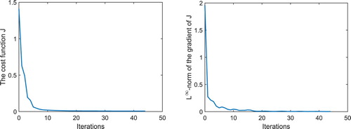
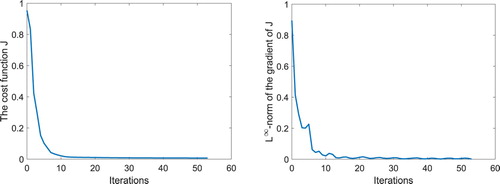
In this example, the Lamé parameters to be recovered are assumed to be constant on Ω and we consider the minimization problem of recovering two scalar parameters. Let $({\lambda }_i,{\mu }_i)\in {\mathbb{R}}^2$ denote the initialization, $({\lambda }_e,{\mu }_e)\in {\mathbb{R}}^2$ the exact parameters to be recovered and $({\lambda }_c,{\mu }_c)\in {\mathbb{R}}^2$ the computed parameters. Table 1 summarizes the computational results of the algorithm. Figures 1–3 show the decrease of the cost function J and the $L^{\mathrm{\infty }}$-norm of $J^{\mathrm{\prime }}$ in the course of the optimization process. The numerical solution represents a good approximation and it is stable with respect to small amounts of noise.

Figure 1. Simulation results for Example 1: History of the cost function J and the $L^{\mathrm{\infty }}$-norm of $J^{\mathrm{\prime }}$ in the case of $\epsilon =0.0$ and $\rho =0.0$.

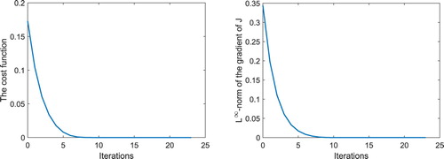
Figure 2. Simulation results for Example 1: History of the cost function J and the $L^{\mathrm{\infty }}$-norm of $J^{\mathrm{\prime }}$ in the case of $\epsilon =0.03$ and $\rho =0.00001$.

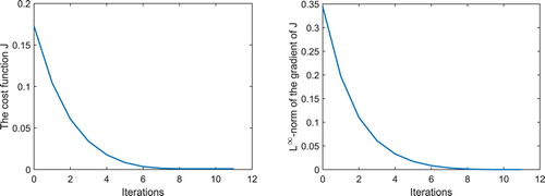
Figure 3. Simulation results for Example 1: History of the cost function J and the $L^{\mathrm{\infty }}$-norm of $J^{\mathrm{\prime }}$ in the case of $\epsilon =0.05$ and $\rho =0.00001$.

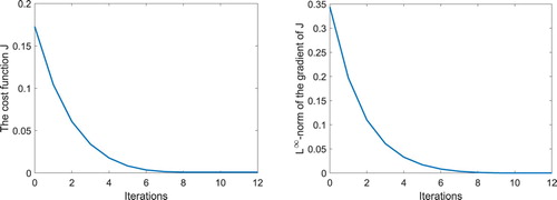
Table 1. Simulation results for Example 1: Reconstruction of constant Lamé parameters.

	$({\lambda }_i,{\mu }_i)$	$({\lambda }_c,{\mu }_c)$	$({\lambda }_e,{\mu }_e)$	${\displaystyle \frac{|{\lambda }_c-{\lambda }_e|}{\left|{\lambda }_e\right|}}$	${\displaystyle \frac{|{\mu }_c-{\mu }_e|}{\left|{\mu }_e\right|}}$
$ϵ=0.0,\rho =0.0$	(1,1)	(2.9999, 6.9999)	(3,7)	3.33e-07	1.42e-07
$ϵ=0.03,\rho =0.00001$	(1,1)	(2.6564, 6.8989)	(3,7)	0.1145	0.0144
$ϵ=0.05,\rho =0.00001$	(1,1)	( 2.6527,6.8869)	(3,7)	0.1157	0.0161

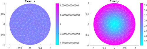
5.1.2. Example 2

In this example, the exact Lamé parameters (Figure 4) to be reconstructed are given by ${\mu }_e(x_1,x_2)=\sqrt{x_1^2+x_2^2}\mathrm{a}\mathrm{n}\mathrm{d}{\lambda }_e(x_1,x_2)=1.$ We reconstruct μ and λ by minimizing the functional (27(27) $J(\lambda ,\mu ):=\sum _{k=1}^4{\int }_{\mathrm{\Omega }}\mathbb{C}(\lambda ,\mu )\hat{\mathrm{\nabla }}(u_N^{g_k}-u_D^{f_k}):\hat{\mathrm{\nabla }}(u_N^{g_k}-u_D^{f_k})\mathrm{d}x+\frac{\rho }{2}{\int }_{\mathrm{\Omega }}\left({\lambda }^2+{\mu }^2\right)\mathrm{d}x,$(27) ) in the space of piecewise constant functions on the FEM mesh. The choice $({\lambda }_0,{\mu }_0)=(0.3,0.5)$ was made as an initial guess.

Figure 4. Simulation results for Example 2: The exact Lamé parameters.

The resulting reconstructions and the absolute errors are depicted in Figures 5–8. The history of cost function J and the $L^{\mathrm{\infty }}$-norm of $J^{\mathrm{\prime }}$ in the course of the optimization process are depicted in Figures 9 and 10. The parameter ${\lambda }_e$ is well reconstructed, while the parameter ${\mu }_e$ is less well reconstructed.

Figure 5. Simulation results for Example 2: The computed Lamé parameters ($ϵ=0.0$ and $\rho =0.0$).

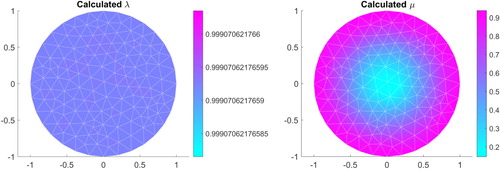
Figure 6. Simulation results for Example 2: The computed Lamé parameters ($ϵ=0.03$ and $\rho =0.0001$).

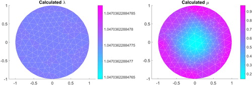
Figure 7. Simulation results for Example 2: Error for λ and μ ($ϵ=0.0$ and $\rho =0.0$).

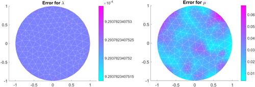
Figure 8. Simulation results for Example 2: Error for λ and μ ($ϵ=0.03$ and $\rho =0.0001$).

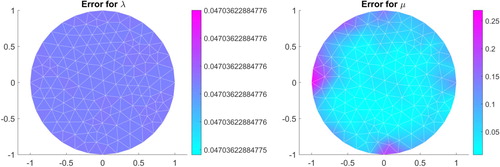
Figure 9. Simulation results for Example 2: History of the cost function J and the $L^{\mathrm{\infty }}$-norm of $J^{\mathrm{\prime }}$ in the $ϵ=0.0$ and $\rho =0.0$.

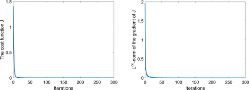
Figure 10. Simulation results for Example 2: History of the cost function J and the $L^{\mathrm{\infty }}$-norm of $J^{\mathrm{\prime }}$ in the case of $ϵ=0.03$ and $\rho =0.0001$.

5.1.3. Example 3

In this example, the exact Lamé parameters (Figure 11) to be recovered are given by ${\mu }_e=\sqrt{x_1^2+x_2^2},$

and ${\lambda }_e=\exp (-5((x_1-1/2{)}^2+(x_2-1/2{)}^2\left)\right)+\exp (-5((x_1+1/2{)}^2+(x_2+1/2{)}^2\left)\right).$ As in Example 2, we reconstruct μ and λ by minimizing the functional (27(27) $J(\lambda ,\mu ):=\sum _{k=1}^4{\int }_{\mathrm{\Omega }}\mathbb{C}(\lambda ,\mu )\hat{\mathrm{\nabla }}(u_N^{g_k}-u_D^{f_k}):\hat{\mathrm{\nabla }}(u_N^{g_k}-u_D^{f_k})\mathrm{d}x+\frac{\rho }{2}{\int }_{\mathrm{\Omega }}\left({\lambda }^2+{\mu }^2\right)\mathrm{d}x,$(27) ) in the space of piecewise constant functions on the FEM mesh, and use the initial guess $({\lambda }_0,{\mu }_0)=(0.3,0.5)$. The resulting reconstructions and the absolute errors are depicted in Figures 5–8. The history of cost function J and the $L^{\mathrm{\infty }}$-norm of $J^{\mathrm{\prime }}$ in the course of the optimization process are depicted in Figures 16 and 17. The parameter ${\mu }_e$ is well reconstructed, while the parameter ${\lambda }_e$ is less well reconstructed. However, the location of the peaks are obtained.

Figure 11. Simulation results for Example 3: The exact Lamé parameters.

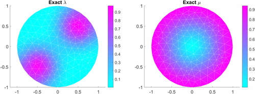
Figure 12. Simulation results for Example 3: The computed Lamé parameters ($ϵ=0.0$ and $\rho =0.0$).

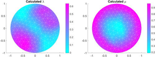
Figure 13. Simulation results for Example 3: The computed Lamé parameters ($ϵ=0.03$ and $\rho =0.0001$).

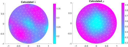
Figure 14. Simulation results for Example 3: Error for λ and μ ($ϵ=0.0$ and $\rho =0.0$).

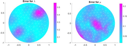
Figure 15. Simulation results for Example 3: Error for λ and μ ($ϵ=0.03$ and $\rho =0.0001$).

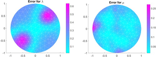
Figure 16. Simulation results for Example 3: History of the cost function J and the $L^{\mathrm{\infty }}$-norm of $J^{\mathrm{\prime }}$ ($ϵ=0.0$ and $\rho =0.0$).

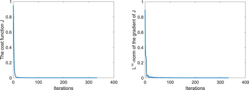
Figure 17. Simulation results for Example 3: History of the cost function J and the $L^{\mathrm{\infty }}$-norm of $J^{\mathrm{\prime }}$ ($ϵ=0.03$ and $\rho =0.0001$).

Remark 5.1

The accuracy of the numerical results presented in this paper depends on the initialization of the proposed algorithm and the choice of the regularization parameter. Meta-heuristic algorithms can be adapted to select a good initialization and avoid being trapped in a local minima. The optimal choice of the regularization parameter is based on some selection methods (such as the discrepancy principle, the generalized cross validation, the L-curve criterion) which is beyond the scope of this paper.

6. Conclusion and outlook

In this paper, we dealt with the identification of Lamé parameters in linear elasticity. We introduced the inverse problem and the corresponding Neumann-to-Dirichlet operator. Based on this, we analysed the connection between the Lamé parameters and the Neumann-to-Dirichlet operator which led to a monotonicity result. In order to prove a Lipschitz stability estimate for Lamé parameters which belong to a known finite subspace with a priori known bounds as well as certain regularity and monotonicity properties, we applied the monotonicity result combined with the localized potentials. The numerical solution of the inverse problem itself, was obtained via the minimization of a Kohn-Vogelius-type cost functional. In more detail, the reconstruction was performed via an iterative algorithm based on a quasi-Newton method. Finally, we presented our numerical examples and discussed them. We want to remark that the monotonicity properties of the Neumann-to-Drichlet operator as well as the results of the localized potentials build the basis for the monotonicty methods for linear elasticity (see [53]).

Disclosure statement

No potential conflict of interest was reported by the author(s).

Correction Statement

This article has been republished with minor changes. These changes do not impact the academic content of the article.

References

- Ammari H, Bretin E, Garnier J. Mathematical methods in elasticity imaging. Princeton (NJ): Princeton University Press; 2015.
- Weglein AB, Araújo FV, Carvalho PM, et al. Inverse scattering series and seismic exploration. Inverse Probl. 2003;19:R27–R83.
- Barbone E, Gokhale NH. Elastic modulus imaging: on the uniqueness and nonuniqueness of the elastography inverse problem in two dimensions. Inverse Probl. 2004;20:203–96.
- Bonnet M, Constantinescu A. Topical review: inverse problems in elasticity. Inverse Probl. 2015;21(2):R1–R50.
- Ikehata M. Inversion formulas for the linearized problem for an inverse boundary value problem in elastic prospection. SIAM J Appl Math. 1990;50(6):1635–1644.
- Akamatsu M, Nakamura G, Steinberg S. Identification of Lamé coefficients from boundary observations. Inverse Probl. 1991;7(3):335.
- Nakamura G, Uhlmann G. Identification of Lamé parameters by boundary measurements. Am J Math. 1993;115:1161–1187.
- Imanuvilov OY, Yamamoto M. On reconstruction of Lamé coefficients from partial Cauchy data. J Inverse Ill-Posed Probl. 2011;19(6):881–891.
- Lin YH, Nakamura G. Boundary determination of the Lamé moduli for the isotropic elasticity system. Inverse Probl. 2017;33(12):125004.
- Imanuvilov OY, Yamamoto M. Global uniqueness in inverse boundary value problems for the Navier-Stokes equations and Lamé system in two dimensions. Inverse Probl. 2015;31(3):46.
- Nakamura G, Uhlmann G. Inverse problems at the boundary for an elastic medium. SIAM J Math Anal. 1995;26(2):263–279.
- Nakamura G, Uhlmann G. Global uniqueness for an inverse boundary value problem arising in elasticity. Inventiones Math. 2003;152(1):205–207.
- Eskin G, Ralston J. On the inverse boundary value problem for linear isotropic elasticity. Inverse Probl. 2002;18(3):907.
- Beretta E, Francini E, Morassi A, et al. Lipschitz continuous dependence of piecewise constant Lamé coefficients from boundary data: the case of non-flat interfaces. Inverse Probl. 2014;30(12):125005.
- Beretta E, Francini E, Vessella S. Uniqueness and Lipschitz stability for the identification of Lamé parameters from boundary measurements. Inverse Probl Imaging. 2014;8(3):611–644.
- Nakamura G, Tanuma K, Uhlmann G. Layer stripping for a transversely isotropic elastic medium. SIAM J Appl Math. 1999;59(5):1879–1891.
- Cârstea CI, Honda N, Nakamura G. Uniqueness in the inverse boundary value problem for piecewise homogeneous anisotropic elasticity. SIAM J Math Anal. 2018;50(3):3291–3302.
- Isakov V, Wang JN, Yamamoto M. An inverse problem for a dynamical Lamé system with residual stress. SIAM J Math Anal. 2007;39(4):1328–1343.
- de Hoop MV, Qiu L, Scherzer O. Local analysis of inverse problems: Hölder stability and iterative reconstruction. Inverse Probl. 2012;28(4):045001.
- Harrach B, Pohjola V, Salo M. Monotonicity and local uniqueness for the Helmholtz equation. Anal. PDE 2019; 12 (7), 1741–1771.
- Harrach B, Lin YH, Liu H. On localizing and concentrating electromagnetic fields. SIAM J Appl Math. 2018;78(5):2558–2574.
- Harrach B. Simultaneous determination of the diffusion and absorption coefficient from boundary data. Inverse Probl Imaging. 2012;6(4):663–679.
- Harrach B, Lin YH. Monotonicity-based inversion of the fractional Schrödinger equation I. positive potentials. SIAM J Math Anal. 2019; 51 (4), 3092–3111.
- Harrach B, Lin YH. Monotonicity-based inversion of the fractional Schrödinger equation II. general potentials and stability. SIAM J Math Anal. 2020; 52 (1), 402–436.
- Gebauer B. Localized potentials in electrical impedance tomography. Inverse Probl Imaging. 2008;2(2):251–269.
- Harrach B. On uniqueness in diffuse optical tomography. Inverse Probl. 2009;25(5):055010.
- Murea C. The BFGS algorithm for a nonlinear least squares problem arising from blood flow in arteries. Comput Math Appl. 2005;49(2-3):171–186.
- Bellassoued M, Imanuvilov O, Yamamoto M. Inverse problem of determining the density and two Lamé coefficients by boundary data. SIAM J Math Anal. 2008;40(1):238–265.
- Bellassoued M, Yamamoto M. Lipschitz stability in determining density and two Lamé coefficients. Mathematical Analysis and Applications J Math Anal Appl. 2007;329(2):1240–1259.
- Harrach B. Uniqueness and Lipschitz stability in electrical impedance tomography with finitely many electrodes. Inverse Probl. 2019;35(2):024005.
- Harrach B, Meftahi H. Global uniqueness and Lipschitz-stability for the inverse Robin transmission problem. SIAM J Appl Math. 2019;79(2):525–550.
- Harrach B. Uniqueness, stability and global convergence for a discrete inverse elliptic Robin transmission problem. arXiv preprint arXiv:1907.02759; 2020.
- Seo JK, Kim KC, Jargal A. A learning-based method for solving ill-posed nonlinear inverse problems: a simulation study of lung EIT. SIAM J Imaging Sci. 2019; 12 (3), 1275–1295.
- Harrach B, Minh MN. Enhancing residual-based techniques with shape reconstruction features in electrical impedance tomography. Inverse Probl. 2016;32(12):125002.
- Harrach B, Ullrich M. Resolution guarantees in electrical impedance tomography. Transactions on Medical Imaging IEEE Trans Med Imaging. 2015;34(7):1513–1521.
- Harrach B, Lee E, Ullrich M. Combining frequency-difference and ultrasound modulated electrical impedance tomography. Inverse Probl. 2015;31(9):095003.
- Harrach B, Minh MN. Monotonicity-based regularization for phantom experiment data in electrical impedance tomography. In: Hofmann B, Leitão A, Zubelli J (eds): New Trends in Parameter Identification for Mathematical Models, pp 107–120. Trends Math., Birkhäuser, Cham, 2018.
- Barth A, Harrach B, Hyvönen N, et al. Detecting stochastic inclusions in electrical impedance tomography. Inverse Probl. 2017;33(11):115012.
- Harrach B, Seo JK. Exact shape-reconstruction by one-step linearization in electrical impedance tomography. SIAM J Math Anal. 2010;42(4):1505–1518.
- Harrach B, Ullrich M. Monotonicity-based shape reconstruction in electrical impedance tomography. SIAM J Math Anal. 2013;45(6):3382–3403.
- Harrach B, Ullrich M. Local uniqueness for an inverse boundary value problem with partial data. Proc Am Math Soc. 2017;145(3):1087–1095.
- Griesmaier R, Harrach B. Monotonicity in inverse medium scattering on unbounded domains. SIAM J Appl Math. 2018;78(5):2533–2557.
- Brander T, Harrach B, Kar M, et al. Monotonicity and enclosure methods for the p-Laplace equation. SIAM J Appl Math. 2018;78(2):742–758. doi: 10.1137/17M1128599.
- Ciarlet PG. The finite element method for elliptic problems. Amsterdam: North Holland; 1978.
- Lin CL, Nakamura G, Uhlmann G, et al. Quantitative strong unique continuation for the Lamé system with less regular coefficients. Methods Appl Anal. 2011;18(1):85–92.
- Gosh A, Gosh T. Unique continuation for a non bi-Laplacian fourth order elliptic operator. arXiv preprint arXiv:1908.05882; 2019.
- Ciarlet PG. Mathematical elasticity, volume I: Three-dimensional elasticity. Series “Studies in Mathematics and its Applications”. Amsterdam: North Holland; 1988.
- Delfour MC, Zolésio JP. Shapes and geometries. 2nd ed. Philadelphia (PA): Society for Industrial and Applied Mathematics (SIAM); 2011. (Advances in Design and Control; Vol. 22). Metrics, analysis, differential calculus, and optimization. doi: 10.1137/1.9780898719826.
- Ekeland I, Temam R. Analyse convexe et problèmes variationnels. Dunod: Collection Études Mathématiques; 1974.
- Correa R, Seeger A. Directional derivative of a minimax function. Nonlinear Anal. 1985;9(1):13–22. http://dx.doi.org/10.1016/0362-546X(85)90049-5
- Lechleiter A, Rieder A. Newton regularizations for impedance tomography: convergence by local injectivity. Inverse Probl. 2008;24(6):065009. 18.
- Dai Y-H. Convergence properties of the BFGS algoritm. SIAM J. Optim.. 2002;13(3):693–701.
- Eberle S, Harrach B. Shape reconstruction in linear elasticity: standard and linearized monotonicity method. arXiv preprint arXiv:2003.02598; 2020.