
 ?Mathematical formulae have been encoded as MathML and are displayed in this HTML version using MathJax in order to improve their display. Uncheck the box to turn MathJax off. This feature requires Javascript. Click on a formula to zoom.
Abstract
In this paper, we propose a novel reconstruction scheme for the low-frequency near-field electromagnetic imaging of high-contrast conductivity distributions inside shielded regions using the system of Maxwell's equations in 3D. In our novel scheme, we focus on estimating the shape characteristics of the electrical conductivity profile inside these regions from low-frequency electromagnetic data measured at external locations for a single frequency. We introduce a colour level set regularization scheme which is a shape-based approach focusing on the simultaneous reconstruction of several shape-like distributions of different conductivity values in the same region of interest. Using two numerical experiments addressing a three-value reconstruction problem related to the imaging of shielded boxes or cargo containers, we compare this novel approach with results obtained from standard voxel-based reconstruction schemes on the one hand and the more established two-value shape-based approach on the other hand. We demonstrate that, depending on the particular situation of the imaging setup, this three-value (or in general multiple-value) shape-based reconstruction technique has the potential to provide superior reconstruction results in many situations, in particular regarding reconstruction of the correct shapes. We also discuss particular challenges of this novel methodology.
1. Introduction
Level set regularization schemes have become a popular methodology when interested in solving shape-based inverse problems. For example, single level set inversion schemes have been designed in a multitude of applications, including non-destructive testing [Citation1–4], reservoir imaging [Citation5–7], medical imaging [Citation8–10], or geophysical prospecting [Citation11,Citation12], amongst others. Its extension, colour level set inversion schemes, have also proven to be useful as they sometimes depict more realistic scenarios. For example, a structural level set method was developed in [Citation13] to detect tumours in breast tissue, a related approach was applied to industrial process tomography in [Citation14], and similar schemes have been developed in the history matching of petroleum reservoirs [Citation15]. Additional level set regularization techniques, such as parametric level sets, have also been used in other imaging modalities such as electrical impedance tomography, see [Citation16–22] for more information.
We focus on developing a scheme to image the contents of boxes and/or containers, using near-field electromagnetic (EM) data. This is a challenging task as the underlying inverse problem is highly ill-posed and the data available is typically limited, resulting in a severely under-determined system. Moreover, shielded containers stop high-frequency EM waves from passing into the contents, through the skin effect. On the other hand, low-frequency contributions to the time signal do have the potential to extract information from inside these shielded regions. The use of low frequency in near-field EM imaging presents an additional challenge of obtaining high resolution reconstructions of material properties in the contents of a shielded container.
In this paper, we introduce a novel colour level set inversion scheme for low-frequency near-field EM imaging to reconstruct material properties inside a shielded region of interest. A special focus is on high-contrast situations where traditional pixel- or voxel-based approaches do not yield satisfactory results due to the inherent smoothing properties of those techniques when using low-frequency data. Those techniques tend to deliver severely low-pass filtered versions of the box content from which it can be impossible to extract sufficient information for detecting or classifying specific objects. In a previous paper [Citation4], a shape-based method as well as a sparsity regularized technique have been proposed in order to better address such a challenging situation. However, whereas both of them perform very well in situations where the content of the domain of interest is mainly composed of two classes of materials with only low variation inside each class, they both struggle to handle other scenarios. For example, when the materials have high contrast with values centred about more than two clearly defined average values. One such situation is the screening of a box or cargo container where there are regions filled with air, as well as moderate and highly conductive material. Classifying such a content into only two classes as implicitly or explicitly done in the sparsity approach or the two-value level set approach does not deliver good results. Therefore, in this paper, we extend the two-value shape reconstruction approach to a multiple-value shape reconstruction approach using more than one level set function for the practical modelling. In particular, we will concentrate on the most prevalent situation of three different classes as indicated in the example given above. This approach is novel in this challenging application and shows surprising results.
The presented colour level set scheme, or its variants, are not limited to low-frequency electromagnetic applications but can be applied to a wide range of tomography problems. This includes X-ray computerized tomography (CT), electrical impedance tomography, microwave medical imaging, and history matching of production data in reservoir characterization. Some currently available work on several of those applications can be found in [Citation13,Citation15,Citation17,Citation20,Citation23,Citation24], and in the references provided there.
It is interesting to compare our application of low-frequency electromagnetic imaging with the above mentioned application of CT, which essentially uses very high-frequency electromagnetic beams (X-rays). In most clinical applications of CT (nowadays using sophisticated sampling geometries) the classical reconstruction algorithms provide high-resolution images [Citation25], such that the combined reconstruction and segmentation approach as followed in our discussion does not on the first view seem to provide significant advantages there. Those CT reconstructions are usually obtained by applying some approximation of the Radon inversion formula, which result in highly efficient implementations, provided that the raw data (so-called ‘sinograms’ or photon counts) are sufficiently complete and of sufficiently high quality (see [Citation25] for details). Therefore, when segmented CT images are needed, a standard CT image is obtained using fast reconstruction techniques, which is then further treated by tailor-made (for example, level set based) segmentation post-processing techniques in order to obtain segmented images [Citation26].
However, even in X-ray CT there are many situations where those quality conditions on raw data are not satisfied. This is the case for example in many industrial settings, but also in specific clinical and biochemical applications where only limited view data or very sparse data are available or desired. In those situations, a combined level set reconstruction and segmentation algorithm, similar to the one proposed here, becomes much more competitive or even superior to standard reconstruction techniques since many classical reconstruction algorithms show significant artefacts which cannot easily be handled by standard segmentation post-processing strategies. For some discussions in the literature addressing such situations we refer to [Citation10,Citation25,Citation27–30].
In the application of low-frequency electromagnetic imaging, there currently does not exist the luxury of a high-resolution reconstruction algorithm (as in X-ray CT) in the first place. Compared to standard X-ray CT images, reconstructions show significantly less details here and interfaces which might be present in the original objects are usually not at all represented in the images obtained from standard reconstruction techniques [Citation31,Citation32]. They need to be enforced by tailor-made reconstruction techniques, making sure that they are in agreement with the physically measured data. The use of a combined ‘reconstruction and segmentation’ algorithm as discussed in this paper seems to be a very natural way of obtaining such segmented images from physical data.
The remaining part of the paper is organized as follows: Section 2 describes the mathematical setup of our low-frequency EM imaging problem with Maxwell's equations. Section 3 formulates the underlying EM inverse problem for recovery of the conductivity value inside the imaging domain and derives some general concepts which are essential for voxel-based and colour level set based reconstruction schemes. As a side product, a voxel-based reconstruction scheme is derived in this section which we use for comparison with the colour level set scheme. Section 4 introduces the colour level set shape-based scheme and formulates the corresponding inverse problem. Section 5 presents a methodology for avoiding certain local minima in the colour level set reconstruction. Section 6 presents two numerical experiments for the colour level set inversion as well as a comparison with alternative regularization schemes (including results using the methodology in Section 5). In this section, we also provide reconstructions which are based on more realistic compositions inside the region of interest in the true phantom with significant internal parameter fluctuations in one of the target zones. Section 7 presents a summary and conclusions of our findings. Lastly, the Appendix explains in details the new tailor-made line search method for our scheme.
2. The near field electromagnetic imaging problem
We model the propagation of EM fields by Maxwell's equations in the frequency domain. These are given as:
(1a)
(1a)
(1b)
(1b) where we assume a time-dependence
for a given and fixed frequency
, with
denoting the imaginary unit and t denoting time. In (Equation1a
(1a)
(1a) ), (Equation1b
(1b)
(1b) ),
denotes the electric field,
the magnetic field,
the magnetic source and
the electric source. The material parameters are
(2)
(2) where
is the electrical conductivity,
is the magnetic permeability and
is the electric permittivity. The index j in (Equation1a
(1a)
(1a) ), (Equation1b
(1b)
(1b) ) indicates that the jth source distribution is considered, where
. Therefore, in our setup, we will consider
different applied sources. These will be modelled in our numerical experiments as rectangular wire loops, but the reconstruction schemes presented here do not depend on this particular choice. The sources give rise to probing fields
and
in (Equation1a
(1a)
(1a) ), (Equation1b
(1b)
(1b) ), which can be measured at the receiver locations. Again, we will use rectangular wire loops as receiving devices, even though the general schemes derived here will work with other measurement approaches with only very minor adjustments. The physically obtained (or in our numerical experiments simulated) measurements are called in the following simply ‘data’, which will be used in order to infer medium characteristics at those places which are not accessible by the antennas.
We are mainly interested here in the non-invasive imaging of the interior of boxes whose walls show a significant conductivity profile. The main difficulty is that EM fields of high frequency do not penetrate sufficiently through such conductive walls due to the well-known skin-effect. Therefore, relatively low frequencies need to be employed which require specialized approaches for data inversion. A possible experimental setup, which is used in our numerical experiments, is indicated in Figure . It also shows a possible distribution of sources and receivers outside the shielding walls. Here, the domain of interest is represented by a cuboid-shaped domain surrounded at all six sides by shielding walls of constant and known thickness. The sources and receivers are distributed uniformly along two planes parallel to the x−y plane each of constant z coordinate. This means that they are opposing each other, separated by the shielded box of interest (see Figure ). Notice that there are no sources or receivers at the other four sides of the box, which limits the aperture of our measurement setup but is more realistic in potential applications such as the fast screening of luggage or cargo containers. We mention again that most of these special assumptions on the geometry can be relaxed in order to arrive at more general imaging scenarios but are sufficient for our proof-of-concept study presented here.
In this paper, we are interested in estimating shapes of the electrical conductivity profile (where ℜ refers to taking the real part of the complex quantity) inside the box from data measured outside the shields. For simplicity, we choose
and
everywhere where
and
represent free space values. This means two of the three material parameters are constant and known throughout the entire domain. We will therefore often refer to the parameter b of (Equation2
(2)
(2) ) simply as ‘conductivity’ in this paper, even though it also contains the known parameter
. In our future research, we plan to address the incorporation of two or three material parameters as space-varying unknowns into the inversion process, but in this study, we will concentrate on the conductivity σ only.
We require a mathematical model of the scenery when doing the inversion. Traditionally, a discretization of the entire 3D domain into a (often rectangular) grid of voxels is the most popular approach for the inversion, where each voxel is assigned a potentially different value of conductivity inferred from data in the inversion process. Following notation from the classical (mainly 2D) literature, we will call this approach ‘pixel-based inversion’, even though it is actually voxels that are assigned values to in our 3D application. In our approach, however, we have chosen to use a completely different model for reasons explained further below. We are interested in imaging situations where some objects of significantly higher conductivity profile are located inside the box surrounded by some background of lower conductivity values, and the task is to identify and characterize those high-conductivity objects from data obtained outside the box. In pixel-based inversion approaches, the classification into different material types is done as a post-processing step, after an inversion has been obtained, by some form of segmentation routine. However, a potential problem occurs here since the classical segmentation post-processing tools, being purely image based but not data based, do not usually verify the agreement of the segmented image with the physically obtained data. Since the modifications which are needed by classical segmentation tools for transforming a very smooth reconstruction into a segmented image are significant in our situations, there is no guarantee that the segmented image still agrees with the measured data the same way as the originally smooth reconstruction.
Therefore, in a previous publication [Citation4], we have proposed a single-level set reconstruction approach which combines the segmentation task and the inversion task into one optimization loop, providing segmented 3D images honouring the physically measured data. In that approach, it is assumed that only two conductivity values are permitted inside the box, namely the high-conductivity value of the object of interest and one single lower value for the background medium. This approach yields reasonable results in many applications. However, there are certain situations where the background medium itself is highly heterogeneous (e.g. consisting of air and some lower conductive materials), such that modelling it by a constant average value everywhere seems to be an oversimplification. In this paper, we extend the previous model to also allow the background medium to obtain two (or even more) different (fixed and suitably chosen) values of a priori unknown distribution. This means, that now in total three (or a specified low number of) different conductivity values are considered for each location inside the box, one for the object of interest and the remaining values for the background. In the inverse problem, we are trying to identify shapes of not too complicated topology which represent distributions of the different materials in the box. During the inversion, each background conductivity value will be classified this way, by implicit means, to belong to exactly one of the corresponding prescribed background material classes. Embedded in this segmented background is the object of interest which corresponds to a separate class representing high-conductivity values. In other words, we perform a simultaneous reconstruction and segmentation of the domain of interest into various different zones which, when we plug the corresponding distribution of material parameters into the forward simulator, reproduces the measured data.
We mention again that this classification can be derived and extended in a flexible way to represent an arbitrary (usually small) number of representative classes. See for example a previous publication related to a different application [Citation13] where a medical setup of higher (microwave) frequency ranges has been treated successfully with more than three parameter classes using a similar scheme, but only in 2D so far. We have tested the use of more than three classes in our numerical experiments (not presented in this paper) also to the low-frequency situation discussed in this paper but have observed that the use of more than three classes does not provide any advantages at this low-frequency regime, mainly due to the lack of resolution inherent to it. Therefore, we will concentrate in this paper on the particular setup of three material classes only. It will become obvious below how to extend our model to incorporate more than three classes in a straightforward way if desired.
In our numerical experiments, we assign a very low value Sm
to the region which represents poorly conductive materials such as air or other essentially non-conductive materials. In addition to this very low conductivity region, there will also be one moderate value representing a class of material at the intermediate regime, and one highly conductive region capturing any materials with significant conductivity properties, all of unknown shape. We emphasize that in our experience it is not very critical which values exactly are taken to represent those classes due to the significant contrast between them. However, in cases where prior information is available indicating the use of specific values this can and should certainly be incorporated in the algorithm by assigning those numbers to the individual classes. A summary of conductivities used in our numerical experiments is described in Table .
Table 1. Conductivity parameters used in numerical experiments.
The shielded walls, which are not part of our level set representation and are modelled explicitly, are here assumed to have a known topology and a moderate conductivity value of Sm
. This assumption will be relaxed in our future work when we incorporate estimation of some characteristics of the shields into the inversion task. An important observation of Table is that the conductivity values range over several orders of magnitude. This is difficult to model with a pure pixel-based inversion model, due to the typical effect of smeared-out values in the reconstructions. In those classical approaches, sharp interfaces between different materials are usually smeared out over large transition zones, which makes the identification of particular regions or shapes extremely difficult or impossible. We will demonstrate this in our numerical experiments.
3. Pixel-based inversion tools
Inverse problems for Maxwell's equations have been investigated for a long time in a variety of applications and settings. For recent overviews of available theoretical and computational results, we refer to [Citation33–35] and the references provided there. The important questions of uniqueness and differentiability of related inverse problems are addressed for example in [Citation36–41]. For derivation of the algorithms in this paper, we assume differentiability (in properly chosen function spaces) of all forward mappings that arise here, allowing us to adopt well-established expressions for the relevant derivatives (or sensitivities) with respect to the unknown medium parameters [Citation35,Citation39,Citation42–46].
The colour level set inversion approach outlined above can be considered a shape-based regularization scheme which provides an alternative to the more classical Tikhonov-regularized pixel-based inversion schemes. As already mentioned, due to the smearing effect related to Tikhonov regularization, the classical Tikhonov-regularization pixel-based scheme is not well-suited for the imaging of high-contrast situations with low frequency EM fields. Nevertheless, both approaches are based on gradient calculations with respect to the continuous parameter-to-data maps, which need to be considered first. Fortunately, most of the results related to this basic ingredient are already well-known, see for example [Citation43,Citation47] or some of the above cited overview articles. Therefore, we will very briefly summarize some of the most important results. These gradient calculations are relevant to both pixel-based and shape-based approaches. They will also provide us directly with a basic Kaczmarz-type pixel-based inversion approach which we will use in our numerical experiments for comparing our novel shape-based techniques with more classical Tikhonov-style schemes.
Let us index the forward operator by each source j, giving rise to the notation . The quantities
,
solve (Equation1a
(1a)
(1a) ), (Equation1b
(1b)
(1b) ) with parameter b and
is a linear measurement operator which might be dependent on the source. Here we take
to behave the same across all sources. In our numerical setup explained further below and in [Citation48], we will formally model measurements at each of the
rectangular closed-loop receiver coils
(
) by
(3)
(3) assuming proper regularity of
. Here,
denotes the tangential unit vector along such a receiver coil. More general linear measurement operators can be used as well without significant modifications of the algorithm. See for example [Citation32,Citation39,Citation44,Citation48,Citation49] for more details and for alternative formulations.
A typical way of addressing the pixel-based inverse problem is to write down a least squares data misfit functional in terms of residual operators. In our case this reads as
(4)
(4) with
, and
being the norm in the data space
.
indicates the true data. Here, the index j refers again to the chosen source distribution. Therefore, the residual operator quantifies the mismatch between model prediction (forward problem) and true data. The cost functional
is useful for monitoring progress of any iterative estimation technique and is often used directly for the design of suitable reconstruction schemes. For example, we can formulate an optimization problem incorporating
with or without additional suitably chosen regularization terms. Many popular minimization schemes use the formal gradient of (Equation4
(4)
(4) ):
(5)
(5) which can be calculated efficiently by a so-called adjoint scheme [Citation42,Citation43]. We refer the reader to these references for a full derivation of the adjoint problem and the gradient of (Equation4
(4)
(4) ). Here, it suffices to quote the result. This is found to be:
(6)
(6) and is given by
(7)
(7) Here, the operator
is known as the adjoint linearized residual operator and the overline on the right hand side indicates to take the complex conjugate. The fields
are taken from (Equation1a
(1a)
(1a) ), (Equation1b
(1b)
(1b) ) and
are obtained by solving a supplementary adjoint Maxwell problem of similar structure as (Equation1a
(1a)
(1a) ), (Equation1b
(1b)
(1b) ) but with using the residual values
as artificial adjoint sources at the receiver locations. For more information on this scheme, see [Citation4,Citation35,Citation42,Citation43,Citation45,Citation46,Citation48].
The non-linear problem described is of large scale in 3D. Usually, iterative techniques are employed for the solution, requiring repeated calculation of descent directions to in (Equation4
(4)
(4) ). Many standard schemes require calculation of the full gradient
in (Equation5
(5)
(5) ). Depending on the available Maxwell solver, this might consume considerable resources and processing time in each iteration. Therefore, alternative techniques have been developed in order to speed up the inversion process. One of those is the non-linear Landweber-Kaczmarz (LK) scheme which is employed here. The optimizer cycles over each source in a certain order and only requires to calculate gradients of partial data sets in each step, which can be done efficiently with the above mentioned adjoint method.
With this single-step scheme it is no longer the primary goal to maximally reduce the data misfit in (Equation4
(4)
(4) ) in each individual step. Instead, in each iteration, we reduce the data misfit
with respect to the jth source only, which needs to be done very carefully in order not to deteriorate too much the data fit regarding the remaining sources. For more information on this general scheme, we refer to [Citation28,Citation42,Citation50–53].
The scheme yields a single-step update formula:
(8)
(8) where we will follow here a sequential rule
for simplicity. Notice that we take the real part ℜ in (Equation8
(8)
(8) ) since we assume that the electric permittivity is known. As already mentioned, choosing the step size τ in this single-step scheme is a difficult problem, and it should be chosen such that updates maintain a balance with the already achieved data fit regarding the remaining sources. Convergence properties of such a single-step approach have been discussed in the literature, see for example [Citation28,Citation52]. A random selection of source positions, leading to variants of stochastic gradient schemes, might provide additional benefits, see for example [Citation54] for related applications in the field of machine learning.
The iteration formula in (Equation8(8)
(8) ) updates the electrical conductivity profile such that it minimizes the cost functional given in (Equation5
(5)
(5) ). This minimization usually delivers quite smooth results due to the specific form of individual updates in (Equation8
(8)
(8) ) but also can contain quite erratic features since in its current form, there are no additional regularization terms, implicit or explicit, included. Therefore, classical regularization approaches often add a Tikhonov-type additional term to (Equation4
(4)
(4) ) in order to stabilize the inversion process. This is usually called ‘Tikhonov regularization’. A similar effect is achieved by keeping (Equation4
(4)
(4) ) unchanged but instead using specifically chosen function spaces. In particular the choice of certain Sobolev spaces enforces higher regularity properties of their members. We will adopt such a Sobolev gradient approach because it does not come with the need for modifying the cost functional (Equation4
(4)
(4) ). In particular, a direct comparison is possible between the results obtained with this approach and those obtained by our colour level set shape reconstruction method, since both are designed to minimize the same data misfit functional but with respect to a different set of optimization parameters.
In the Sobolev gradient approach, we assume that the quantities of interest (say, u, v) are members of a Sobolev space equipped with the
norm
and inner product
with suitable boundary conditions, see for example [Citation3,Citation4,Citation9,Citation11,Citation24] for more details. In our numerical experiments, we will choose
and select
empirically in order to achieve a stable reconstruction process. Since the gradient operator depends on the spaces and corresponding inner products, we have to calculate new expressions for the corresponding gradient directions. Fortunately, as shown in [Citation3,Citation4,Citation9,Citation11,Citation24], the Sobolev gradient expressions
can be obtained in a straighforward way from the
based gradients (Equation6
(6)
(6) ), (Equation7
(7)
(7) ) by simply projecting these expressions into a smoother space using the following recipe
(9)
(9) Here, I is the identity operator and Δ is the Laplacian operator. Solving (Equation9
(9)
(9) ) to obtain
provides us with a smoothed gradient for the inverse problem. For derivation of (Equation9
(9)
(9) ) and for more information on practical ways of calculating this smoothed gradient, we refer the reader to a more detailed discussion in [Citation3,Citation4,Citation9,Citation11,Citation24].
4. Colour level set shape-based inversion
Level set shape-based reconstruction methods provide an alternative to pixel-based schemes and have been applied in many areas [Citation23,Citation24,Citation47,Citation55–57]. Level set methods provide additional regularization to the inverse problem as they combine parameter values into a small number of classes with fixed (or simultaneously estimated) representative values. This way level set based schemes solve two tasks at the same time: reconstruction of physical profiles from physically measured indirect data and the segmentation of that profile into a small number of classes. The most basic of those schemes, here called standard level set method, assumes that the domain is composed of exactly two different classes of fixed parameter values. They have been shown to perform well in certain situations of low-frequency EM inverse problems [Citation1,Citation4,Citation7,Citation11,Citation23,Citation24]. However, in some scenarios, for example, when multiple conductivity values of significantly different magnitudes are present in the domain, standard level set methods are not optimal (neither are pixel-based inversion schemes). In such scenarios, colour level set methods can be applied in an attempt to deal with such more challenging situations.
We refer to the theory of standard level set methods, in particular with respect to the application considered here, to a previous publication [Citation4]. In the following, we directly turn our attention on the extended setup necessary for handling more than two different regions by a certain number of level set functions. A very general introduction to multiple shape reconstruction by a variety of practical level set based approaches can also be found in [Citation23,Citation24].
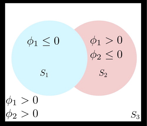
For modelling three different regions, we will be using here two different level set functions. Therefore, we begin by introducing two sufficiently smooth level set functions , such that
(10)
(10) where
and
are the corresponding parameter values (the superscripts not to be confused in the following with powers of b which are not needed in this study).
A similar but conceptually different multiple level set model has been introduced originally for the application of image segmentation in [Citation58] where two level set functions are used for describing four different regions. In contrast to the model used in [Citation58], our representation (Equation10(10)
(10) ) uses two level set functions in order to only model three different regions. Moreover, our model is not completely symmetric in the three values
in the sense that
exclusively specifies the region filled with
, whereas the sign of
by itself does not provide sufficient information about which value to choose. See Figure for a visualization of this situation. This hierarchical arrangement actually provides some advantages compared to the model proposed in [Citation58] when applied to shape reconstruction problems from indirectly obtained data.
One of its advantages is that it allows us in a very convenient way to introduce single new regions at any stage of the reconstruction process into the model without the need of redefining the representation of already existing regions. We just add one additional level set function which will specify a new region without the risk of ambiguity. For example, a reconstruction could start from just using during early sweeps, segmenting the domain into only two regions, and at a later stage could branch out by adding
in order to refine the segmentation.
Another advantage is that two regions usually do not have a point-like (or cusp-like) interface with each other (except of some very unlikely special situations). Instead, two different regions normally share a full curve-like interface in 2D or a full surface-like interface in 3D, which makes it easier to apply the concept of shape velocity and shape gradient for shape propagation or their ‘narrowband analogon’ as it is outlined further below and used in this paper. Notice also that our scheme extends accordingly when more than two level set functions are used in order to model more than three regions and avoids some local minima which can occur with some other schemes of using multiple level set functions [Citation23,Citation24].
In general, all three profiles can be either smoothly varying functions in these regions or can be taken as constants. In our numerical experiments and in the notation of this paper, we only consider the latter choice. An equivalent way of writing the conductivity profile in (Equation10
(10)
(10) ) is
(11)
(11) where
is the Heaviside function.
With the colour level set representation of the electrical conductivity profile formally defined, we now introduce the relevant data misfit and cost functional:
(12)
(12) (and similarly the quantities
and
as in (Equation4
(4)
(4) )). We are now interested in finding a suitable
such that the data misfit
is minimized. Notice that, even though using the same symbol as in the pixel-based case for simplicity in the notation,
is now assumed to be a function of
.
When comparing with more traditional colour level set approaches for image processing, we would like to point out here that the cost functional (Equation12(12)
(12) ) for our colour level set inversion method still contains the data-to-model mapping
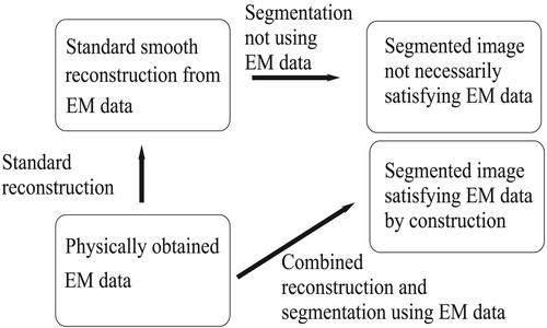
in its formulation. Image post-processing applications usually replace this (physical) data fidelity term by a term measuring proximity to a reference image [Citation26,Citation58] as outlined in Figure . We cannot rely on any reference image in our application but only on the physically gathered data.
Figure 1. Comparison of the traditional 'first reconstruct then segment' scheme with the proposed 'simultaneously reconstruct and segment' scheme. The results on the right hand side are both segmented images, of which only the one from the simultaneous approach is guaranteed to satisfy the physically obtained EM data.
With (Equation5(5)
(5) ) and (Equation6
(6)
(6) ), and by applying formally the chain rule for differentiation with respect to
, we obtain an expression for the gradient of the colour level set cost functional:
(13)
(13) where
(14)
(14) and
(15)
(15)
(16)
(16) Here, the notation
refers to the partial derivative with respect to that level set function, ℜ indicates again to take the real part in order to account for real-valued level set functions, and
denotes the Dirac delta distribution. Evaluating those expressions (Equation14
(14)
(14) ) requires us to solve one adjoint Maxwell problem for each index j in order to obtain
. In the advent of numerical experiments,
has to be approximated by a function in a suitable space, since it is not well defined on a numerical grid. Therefore, we choose to use already in this theoretical derivation a narrowband function as an approximation to it [Citation59,Citation60], such that
, where
(17)
(17)
and
is the characteristic function. Notice that this approximation conserves the descent direction property of the (negative) gradient for small values of
, which is all we need for implementing our descent scheme. In the general case, we assume that boundaries of objects are smooth. Therefore, each component in the gradient from (Equation14
(14)
(14) ) is projected to a smoother space using the recipe in (Equation9
(9)
(9) ) and is denoted accordingly by
. The resulting gradient is now a sufficiently smooth function well-defined on the entire domain Ω which can be used for updating the level set function
everywhere. We mention that the process of extending the Dirac delta to a smooth function on the entire domain is reminiscent of finding an ‘extension velocity’ for classical level set applications in computational physics [Citation60]. Indeed, a similar interpretation can be obtained in our case [Citation23,Citation24]. This leads to the LK-single-step iteration formula:
(18)
(18) where the step size is
and
denotes the Hadamard (element-wise) product. When using non-linear LK schemes in single-level set inverse problems, choosing the step size has proven to be tricky [Citation3,Citation4]. However the line search scheme devised in [Citation4] was shown to be successful, therefore, we adopt the criterion developed there and extend it to the colour level set regime. Note that the parameter s denotes the current sweep number, which increases by once when we have computed an update for all sources.
The line search essentially uses a backtracking scheme which does not require any additional solves of the forward or adjoint problem. It controls the number of interior voxels whose conductivities change per iteration. A sufficiently large line search parameter τ is chosen and reduced until a smooth evolution of the shape is guaranteed. This amounts to counting the number of voxels that change value based on the current step size, then reducing it until the number of voxels that change value is inside an admissible interval. An outline of the scheme in a generalized colour level set setting is given in Appendix, where we apply the criterion for a particular case.
5. A stochastic seeding process
We mentioned above that the colour level set scheme (Equation10(10)
(10) ), (Equation11
(11)
(11) ) helps avoiding certain local minima. However, shape evolution schemes with more than two values still suffer from a particular type of local minima due to the nature of only moving interfaces locally.
In particular, certain local minima are associated with the incorrect classification of isolated objects embedded in a background region as being composed of material associated with region
instead of region
, or vice versa. This situation does not occur in standard level set applications where only one background profile and one possible inclusion value are used. We will demonstrate this ambiguity in our numerical experiments.
In order to deal with that type of local minima, we introduce a stochastic seeding process which improves the situation to a certain degree. Unfortunately, due to the high degree of ill-posedness of this inverse problem, and the poor resolution resulting from it, this problem cannot be completely avoided.
The general idea is to randomly place small objects, alternating between type and type
, into the domain in order to let the algorithm decide whether such an object can favourably replace the already existing structures. Therefore, this strategy can be considered as a way of probing at different stages of the algorithm different variants of ‘advanced initial guesses’, with the hope that the algorithm will select the one leading to the global minimum. Since the entire shape evolution does take a significant number of iterations also without this seeding, such an embedded probing is more efficient compared to starting the entire reconstruction algorithm with a large number of different initial guesses in an ensemble type approach [Citation61]. It still adds computational expenses to the reconstruction, and we will investigate in this paper amongst others whether this additional cost is rewarded by the results or not. For similar stochastic seeding algorithms in a completely different level set reconstruction problem, and employed for different reasons, we refer the reader to the publications [Citation5,Citation6,Citation15,Citation62]. In the following, we very briefly outline the general approach including some technical aspects of it.
Let us assume that we want to place an object centred in a small region . This amounts to lowering the level set function until it is negative in the desired region, forming a new object. Since our numerical experiments use a much coarser grid compared to [Citation5,Citation6,Citation15], we will only consider two regions:
and
, such that
, where
is the domain containing a seeded object and
is its complement. Whilst an additional interim region of smoothing the level set function between
and
would be useful, in our application we will not consider this additional region due to the coarseness of the grid in 3D. Placing an object in
is practically achieved by solving the following supplementary minimization problem on the corresponding level set function φ at selected steps of the colour level set reconstruction:
(19)
(19) where
are suitably chosen weighting parameters,
and
and
are characteristic functions concentrated on the domains
and
, respectively. The minimizer of this cost functional,
, replaces the level set function
. The first term in the cost functional is a penalty on the distance between new and old level set functions in the domain outside the seeded region (
) and the second penalizes distance between the desired minimizer
and some negative μ inside
. A desired smoothness of the resulting level set function is obtained by searching for the minimizer inside a suitably chosen Sobolev space
, as introduced in Section 3.
We minimize the cost functional in (Equation19(19)
(19) ) for randomly selected locations for
at different steps of our colour level set inversion routine, but only during a specific range of iteration numbers which defines the seeding phase. This process is external to the actual colour level set inversion routine and can be seen as off-line iterations which are performed either before or after selected updates for
. In context of the level set functions themselves, all we want to achieve in those external iterations is to approximate a given value by the level set function inside the seed region
, with minimal changes outside of it.
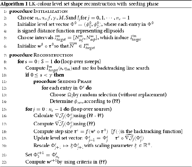
We summarize the new shape-based reconstruction approach discussed so far in form of a pseudo-code in Algorithm 1.
6. Numerical experiments
In this section, we will demonstrate the performance of this novel algorithm in a number of different situations, and compare it with a selection of alternative algorithms. In particular, we want to use the LK-colour level set scheme in Algorithm 1 for the application of imaging shielded regions. We choose to model the entire experimental domain as a cube-shaped region which includes a shielded container of size
, similar to the situation depicted in Figure . As indicated in that figure, the regions of heights 0.3m above and below the container are reserved to accommodate the (source and receiver) antennas. The walls of the container are 0.3m thick at each side. We discretize this experimental domain
by using a regular
rectangular grid, each grid cell having physical dimension
. This means that the actual container including shields occupies
grid cells. The internal region of the container without the shields is represented by
grid cells, which amounts to a total of 6144 grid cells. Those are the locations where the physical parameter (conductivity) needs to be specified by the algorithm. In order to do so, we consider a number of
sources and
receivers, with all sources and receivers representing wire loops as indicated as well in Figure . Each source and receiver has dimension
, with the sources being excited with an electric current
and each receiver recording a data value represented by (Equation3
(3)
(3) ). A fixed and given probing frequency of f = 1MHz is applied in all cases.
Figure 2. Opposing arrays of sources and receivers with shielded cage in between. The interior of the box is hidden behind the shields. The sources and receivers are only located on top and bottom of the box, but other setups are also possible. Left: Complete set up of imaging the contents of a shielded cage. Right: Schematic of shielding in z direction. The domain of interest is between these shields in each direction.
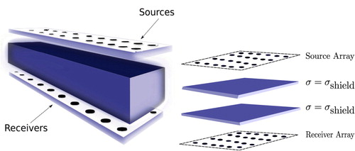
Figure 3. 2D Visualization of level set representation described in (Equation10(10)
(10) ); In this schematic visualization, it is assumed that the individual regions
and
are both disc-shaped, but that the specific rule (Equation10
(10)
(10) ) specifies which value to take in the overlap region
On a more technical note, the computational domain is furthermore surrounded in our computational setup by additional absorbing boundary layers in order to prevent any outgoing fields from being reflected back into the computational domain. Our discretization of Maxwell's equations in (Equation1a(1a)
(1a) ), (Equation1b
(1b)
(1b) ) follows closely the scheme described in [Citation63–65] and has been implemented for our purposes in Python. It is a finite volume method using a Yee grid which is well suited to deal with high-contrast situations as the ones considered here. It solves for the EM fields
and
indirectly via finding a vector potential solution. The discrete Maxwell system is iteratively solved using the BiCGSTAB algorithm, following advice from [Citation66], with a tolerance
. For more details on the numerical code for solving Maxwell's equations in our numerical experiments, we refer to [Citation48].
Here we demonstrate the performance of Algorithm 1 by using two numerical experiments, both of which involve placing two objects with differing constant conductivities in a background conductivity profile resembling air. The first is an object embedded inside another, whereas the second consists of two isolated objects. Both examples come with particular challenges.
In all numerical experiments, we choose this domain of interest to be shielded by a closed solid cage with conductivity of the walls being Sm
. Currently, a level set representation is not used for the shields since they are assumed to be given and known. These are added to the conductivity profile once it has been defined by
and
, for both data generation and when the level set functions are updated. As a default, we initialize both level set functions in the vector
as ellipsoids in the central area of our domain (but not identical). This initial guess is by far not optimal and better initializations can be designed by simple preprocessing steps. However, for our purpose, an almost centred initial guess for each level set function suffices for demonstrating the general behaviour of the algorithm. Specific values for the conductivities used in the two numerical experiments are shown in Table .
Table 2. Conductivity parameters used in numerical experiments.
In all our numerical experiments presented in this article, we choose to use synthetically generated data using the same forward modelling method, with additional noise added in the form of white Gaussian noise (1%). Therefore, the data admits a decomposition
(20)
(20) where
is the electric field generated by the true objects in each numerical experiment,
is given by (Equation3
(3)
(3) ),
and
is a scaling parameter representing the noise level. In both numerical experiments we assume the computational setup described above and that the measured data
used for recovery follows the form described in (Equation20
(20)
(20) ). Notice also that, in order to avoid the so-called ‘inverse crime’, we have included three different variations of the first numerical experiment where one of the background distributions occupying one of the regions is perturbed by different types of additional (including non-Gaussian) noise. We will comment on that further below. In our future work, we plan to use data generated by different grid sizes and/or different forward solvers, but for our proof-of-concept study presented here, we are confident that adding Gaussian noise fits the same purpose and allows us to evaluate better the quality of the final reconstructions against more traditional inversion schemes.
6.1. LK-colour level set inversion for numerical experiment 1
We refer to Appendix for details on the particular values chosen for the line search scheme. Even though the line search criteria are quite technical, they form an important part of our reconstruction algorithm. Therefore, along with images of the colour level set reconstruction, we also display information on the step size in relationship with the average number of voxels that change per sweep and information on how the pseudo-cost behaves (the concept of a pseudo-cost is defined further below when discussing Figure in more detail). In the corresponding Figure displaying the step size information, we display the admissible interval range as solid straight lines (with black colour in the online version of this paper), and bounds of the desired region
are shown in dashed straight lines (with green colour in the online version).
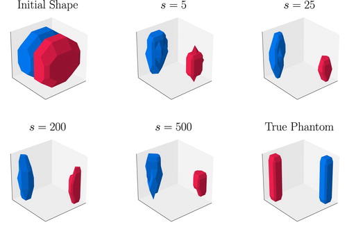
Figure shows various stages of a 3D LK-colour level set inversion for the Numerical Experiment 1 in form of surface plots. The bottom right image displays the true phantom, and the upper left image shows the initial guess. The remaining images display snapshots of the shape evolution at various sweep numbers (each sweep considering all source positions exactly once). Cross-sections of the final result are also displayed in the fourth row of Figure which will be discussed further below. It becomes visible that, upon convergence, the algorithm has managed to capture the main topological characteristics of the true phantom, even though we have by far less data available than we have pixels with unknown conductivity values. This is even more impressive considering that each of the three conductivity regions present in the true phantom has quite a high contrast with respect to the others.
Figure 4. Surface plots of 3D shape evolution for Numerical Experiment 1. Shown are the initial shape and snapshots at iteration numbers and the true phantom. The surrounding shields are not shown here. In the online version of this paper, the colour red indicates the shape of the conductivity
and blue indicates the shape of the conductivity
. The third region is transparent and represents air (
).
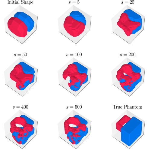
Figure 5. Line search analysis of LK-colour level set reconstruction for Numerical Experiment 1. Top row: Evolution of the average number of voxels as a function of the sweep number s. The dotted (and yellow in the online version of the paper) line represents
and the solid (black in the online version) line represents
. Middle row: Evolution of the step sizes
and
, denoted in the online version by yellow and black lines. Bottom row: Evolution of pseudo-cost
as a function of the sweep number s.
![Figure 5. Line search analysis of LK-colour level set reconstruction for Numerical Experiment 1. Top row: Evolution of the average number of voxels N¯ as a function of the sweep number s. The dotted (and yellow in the online version of the paper) line represents N¯s1 and the solid (black in the online version) line represents N¯s2. Middle row: Evolution of the step sizes τ1s and τ2s , denoted in the online version by yellow and black lines. Bottom row: Evolution of pseudo-cost J~[Φ]s as a function of the sweep number s.](/cms/asset/1b8f1a73-cd4c-4bb9-9996-e074e81cd1de/gipe_a_1797003_f0005_oc.jpg)
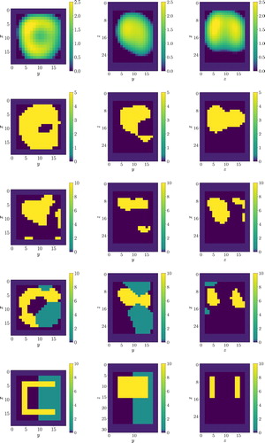
Figure 6. 2D cross-sections through a 3D reconstruction for Numerical Experiment 1 using different regularization schemes. Shown is the container region including shields. Each row: Left z = 25, middle , right y = 18. 1st row: LK-Pixel, 2nd row: LK-single-level set
, 3rd row: LK-single-level set
, 4th row: LK-colour level set and 5th row: true phantom.
Compare already here the corresponding evolution of line search criteria and cost functional displayed in Figure (discussed further below). As expected, the reconstruction cannot be perfect even though the value of the cost functional has been reduced significantly by sweep s = 500. Based on the above count of unknowns and data, one expects some form of non-uniqueness in the reconstructions which cannot be removed without additional prior knowledge. Indeed, the final reconstruction shows a higher amount of fine details compared to the true phantom. Some smaller parts of value are attached to the main body of value
. This appears to be an artefact that stems from details of the shape evolution and can be characterized as a typical local minimum. Removing those artefacts would not make a significant change in the final cost. On the other hand, it is comforting to observe that the annulus in the region of
is correctly identified, even though it is not included in the initial guess. Overall most of the material with values
and
are contained in the correct area of the container when compared with the true model.
Figure shows reconstruction information of Numerical Experiment 1. In the top figure, we observe the average number of voxels that change each sweep for both level set functions (dotted line (yellow in the online version): , solid line (black in the online version):
). The top solid straight line descends as the algorithm progresses, making the admissible interval smaller. This induces
to also be smaller, meaning acceptance of an update is more difficult.
Rather than monitoring the actual cost, which is computationally demanding, we choose to track a different measure which is cheap to compute. As indicated in Algorithm 1, let s denote the sweep number, j the index of the source position and the corresponding cost value as calculated according to (Equation12
(12)
(12) ) in order to obtain the next update. The pseudo-cost
and actual cost
, both obtained upon completion of sweep number s, are defined as
(21)
(21) The actual cost
corresponds to the standard cost value evaluated off-line by using the last level set function obtained by sweep s. Its calculation requires us to run
forward problems using our Maxwell solver on this single-level set function. The pseudo-cost
, on the other hand, uses partial cost values associated with the level set functions that are calculated by Algorithm 1 during sweep s in order to obtain the individual updates. Its calculation comes without any significant additional expenses. It can be viewed as a lagged cost and is significantly less expensive to obtain than computing the actual cost
after each sweep. When adopting our line search strategy, significant differences between the pseudo and actual cost have not been observed throughout the evolution when choosing to calculate both in the numerical experiments. Therefore, only
is calculated and displayed here.
In this particular example, now observing the middle figure, we see that the algorithm has managed to find a step size which allows for the majority of sweeps. The bottom figure shows the pseudo-cost in each sweep, which decreases as the algorithm progresses, meaning the error between the data generated by our reconstruction and the test phantom is becoming smaller.
6.1.1. Comparison of regularization schemes
Figure shows a comparison of the colour level set inversion scheme with other reconstruction algorithms for Numerical Experiment 1. As part of this, we compare our colour level set reconstructions with two variants of a single-level set inversion and also a traditional -pixel-based scheme. The two single-level set inversions differ in their a priori information; the first (diplayed in the second row of the figure) assumes that the single interior conductivity value in the single-level set inversion, which we label
, is an arithmetic average of the two different values present in the true phantom. The second (displayed in row three of the figure) assumes that it coincides with the highest of the two values, namely
. The exterior background in both these cases is assumed to be
, as in the colour level set approach.
The figure moreover shows in row one that the -pixel-based scheme performs reasonably well given that the true phantom has relatively high contrast between conductivity domains. This reconstruction roughly corresponds to the upper left panel of the flow chart provided in Figure . It satisfies the data but lacks the clear structure suggested by our a priori information. It can be argued whether applying a standard off-the-shelf image segmentation approach to the standard Tikhonov Philips type result shown in row one of this Figure would be a good approximation to the correct reference figure, which is shown in row five of the same figure. As mentioned before, the pixel-based scheme promotes over-smooth conductivity profiles in low-frequency situations, whereas in contrast the level set inversion schemes enforce non-smooth conductivity profiles with sharp edges. When given correct a priori information on conductivity values, the level set inversion can resolve interfaces between shapes more clearly.
However, in this more challenging case, the binary approach using just one level set function clearly might not be the best possible approach either, as seen in rows two and three of the figure. Apparently, more complicated scenarios such as the true phantom for Numerical Experiment 1 do not lend themselves well to the single-level set inversion, since fundamentally the method is designed to only recover shapes of two-parameter domains. This observation motivates the extended studies performed in this paper on employing more general colour level set schemes instead.
But before examining results of the novel colour level set approach, let us compare two values for in this a priori incorrectly designed level set model. As shown in [Citation4], using an incorrect value for the level set inversion tends to deliver growing or shrinking domains to fit the data depending on whether a priori information on the conductivity is lower or higher than what is present in the true phantom. We observe this phenomenon in the LK-single-level set reconstruction here. When we take the interior conductivity value to be an average of the two present in the true phantom, we observe an inflated or deflated conductivity profile as the algorithm tries to adjust the shape to fit the data. We can compare this situation to the second scenario, where we take the interior conductivity value to be the highest interior value present in the true phantom. With this choice, we obtain a much smaller interior shape since the interior conductivity is almost double that of the averaged interior value.
The results of the LK-colour level set inversion algorithm, shown in row four of the Figure , demonstrate that this novel scheme performs much better than the standard level set approach (and also better than the pixel-based approach) in attempting to recover the true phantom. This is so since characteristics of the true phantom are present in the reconstruction. For example, the scheme has managed to recover a conductivity profile that has the same distinctive separation features (i.e. a portion of is trapped in between
and
). In comparison, the pixel-based scheme delivers a smooth conductivity profile extended over the entire domain, and the single-level set scheme delivers an inflated or deflated shape (depending on the single internal value used) of the true phantom.
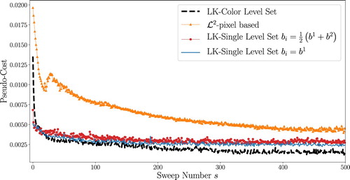
Figure shows a comparison of the pseudo-cost for each reconstruction scheme shown in Figure . The -pixel-based scheme has the highest data misfit value, whereas the data misfit of both single-level set schemes are relatively close to the colour level set scheme despite poor recovery of the true phantom. The relatively high value for the pixel-based scheme is a little bit surprising, but can be due to very slow convergence of this scheme. Displayed is the value after s = 500 sweeps, but it is possible that further reduction is achieved by keeping the scheme running significantly longer (which however would be impractical in realistic applications). It might also be due to the smoothing effect of the pixel-based reconstruction schemes, which makes it difficult to correctly fit data obtained with a high-contrast model from reconstructions of very low contrast. The two-value level set approach performs better here, but still cannot match the low final cost value of the colour level set reconstructions in this example. This is certainly plausible, since the (three-value) colour level set model agrees best of all with the correct setup of the true phantom and incorporates optimally the available prior information.
Figure 7. Pseudo-cost for four different regularization schemes; LK-colour level set, LK-single-level set, LK-pixel and SD-pixel.
6.1.2. Variability in the true conductivity profile
We can test the numerical stability of the colour level set scheme by increasing the realism of the true phantom inside the container. In this case, we assume that the background conductivity (other than air which is
) has some variability. Here, we assume that the true conductivity profile admits the following decomposition:
(22)
(22) where
is drawn from a probability distribution and the
superscript denotes the (discretized) true level set function. In other words, the parameter content of region
is actually random with properly chosen statistical characteristics, to be explained below. Those distributions are chosen to depict possible variations of actual boxes or cargo containers in realistic situations. Here we will consider a comparison between two variations of a normal distribution N and a uniform distribution U for the true content of region
. Therefore, in the two cases,
admits the decompositions
(23a)
(23a)
(23b)
(23b) where
are chosen parameters. Note that our two variants of drawing from a normal distribution in (Equation23
(23a)
(23a) ) stem from choosing various α which determines the variance.
Numerically speaking we now assign each cell in of the true phantom to a single draw from a probability distribution without replacement. We consider three examples; the first where
is drawn from a normal distribution such that the conductivity associated with
is now slowly varying around
; the second where
is drawn from a uniform distribution whose mean is
; and the third where
is drawn from a normal distribution with mean
. See Figure .
Figure 8. Left: Sample of conductivity profile in using probability distribution
, Middle: Sample of conductivity profile in
using probability distribution
, Right: Sample of conductivity profile in
using probability distribution
.
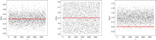
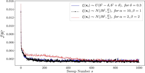
Figure shows the statistical samples generated for building the true conductivity profiles associated with used in the inversions depicted in Figures – , from left to right, respectively. In all three figures, the horizontal (red in the online version) line denotes the value of conductivity
which is used in the colour level set inversion scheme.
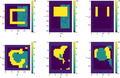
Figure 9. 2D cross-sections through a 3D reconstruction for Numerical Experiment 1 using the formulation in (Equation22(22)
(22) ) for the true phantom. Here,
is drawn from a normal distribution with parameters
. Each row: Left z = 23, middle x = 15, right y = 18 Top: true phantom, Bottom: LK-colour level set reconstruction at sweep s = 1000.
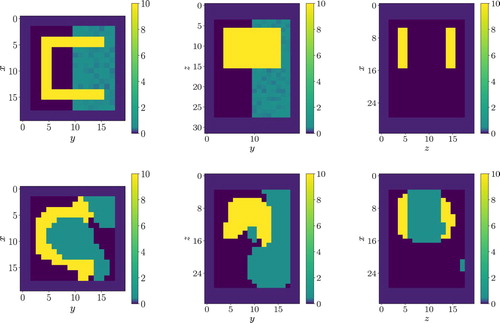
Figure 10. 2D cross-sections through a 3D reconstruction for Numerical Experiment 1 using the formulation in (Equation22(22)
(22) ) for the true phantom. Here,
is drawn from a uniform distribution with parameter
. Each row: Left z = 23, middle x = 15, right
Top: True Phantom, Bottom: LK-colour level set reconstruction at sweep s = 10000
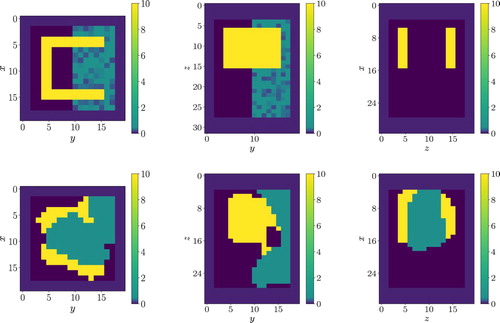
Figure 11. 2D cross-sections through a 3D reconstruction for Numerical Experiment 1 using the formulation in (Equation22(22)
(22) ) for the true phantom. Here,
is drawn from a normal distribution with parameters
. Each row: Left z = 23, middle x = 15, right y = 18 Top: true phantom, Bottom: LK-colour level set reconstruction at sweep s = 1000.
Let us now apply the colour level set inversion scheme to this new challenging situation where content in the region is still assumed constant during the reconstruction, reflecting our lack of knowledge of the detailed nature of the content inside the box. Figures – depict LK-colour level set reconstructions where the true
is characterized by using draws from both normal and uniform distributions.
All three figures show a LK-colour level set reconstruction where the region in the true phantom has a significant variability of internal conductivity associated with it. In comparison to the reconstructions shown in both Figures and , we see that the reconstruction of
is no longer occupying significant parts of the central region between the structures described by
and
(representing a gap filled with air in the true phantom). However,
still has resemblance with the true phantom and some characteristics remain from the reconstruction involving a constant conductivity profile associated with
.
Apparently the samples shown in the left and middle images of Figure do not inhibit the LK-colour level set inversion in its recovery of the shape in Figures and since values in fall either side of
. One possible explanation of this behaviour is that the underestimation and overestimation of the conductivity associated with
in the colour level set inversion effectively cancel each other out when observing the data (the growing and shrinking effect as discussed earlier), since both these reconstructions are very similar to that shown in Figure .
In contrast, the conductivity reconstruction in Figure associated with for the level set inversion using the sample in the right image of Figure does not perform as well as the others. Even though the reconstruction overall captures the true behaviour of the conductivity profile, its resemblance to the true phantom is slightly worse than the other two sampling techniques, as it should be expected. This most likely occurs because the a priori information given to the algorithm overall underestimates conductivity values in large parts of the domain. Though it is encouraging that even in penalized situations like this the algorithm can still capture many characteristics which are truly present.
Nevertheless, all three reconstructions are impressive considering many of the conductivity values associated with are not used as a priori information in the LK-colour level set reconstruction. Figure , for example, shows a LK-colour level set reconstruction of a true phantom whereby the conductivity profile associated with
has large variability and has mean around twice the true value. Although the reconstruction scheme has been heavily penalized with wrong a priori information, the recovery is quite similar to the first two, which is impressive.
Figure shows a comparison of the pseudo-cost for each sampling technique.
Figure 12. Pseudo-cost comparison between different sampling methods for creating conductivity profile associated with .
6.2. LK-colour level set inversion for numerical experiment 2
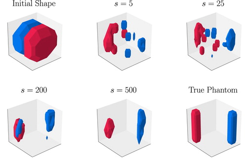
After the very convincing results seen in Numerical Experiment 1, we want to present now a different setup which highlights some potential pitfalls of the newly proposed algorithm. We also present a way of circumventing those maybe unexpected difficulties. In a similar way as for Numerical Experiment 1, Figure shows various stages of a 3D LK-colour level set reconstruction for Numerical Experiment 2. The general setup of this example is similar to the one in Numerical Experiment 1, but the true profile (shown in the bottom right image of Figure ) is quite different here with both objects being separated by a very large distance.
Figure 13. Surface plots of 3D shape evolution for Numerical Experiment 2. Shown are the initial shape and snapshots at iteration numbers and the true phantom. The surrounding shields are not shown here. In the online version of this paper, the colour red indicates the shape of the conductivity
and blue indicates the shape of the conductivity
.
By observation, the algorithm performs well in the sense of locating both objects inside the imaging domain. However, the classification of the objects is obviously biased by choice of the initial guess and is done incorrectly in this particular reconstruction. This is problematic in situations where the exact nature of the recovered objects is of importance. Notice that this incorrect classification is compensated by the algorithm because it provides inflated or deflated areas for each of the two conductivity domains as a result of optimally fitting the cost functional.
We mention here without showing this result (for the sake of brevity), that if the initial guess is flipped, in the sense that was changed to
and vice-versa, we recover the correct classification and location as it might be expected. Accordingly, choice of the initial guess can significantly influence the final reconstruction in the colour level set approach, even more than it is usually seen in the classical two-value level set method. This indicates that expectations on distinguishing between all regions correctly should not be set too high in this approach. The reconstructed internal values at each location can be affected by a new type of local minima in the chosen optimization approach, not present in the other methods discussed in this paper. We emphasize, though, that reconstructions using the colour level set scheme still seem at least of the same quality and usefulness as the more traditional methods compared to in this paper. None of those would be able to correctly identify the actual contrast to the background of each object.
Certainly, some of the previously emphasized additional advantages of our novel scheme are not guaranteed here and depend on choice of the initial guess. Certainly, remedies are available and we will present one suggestion using random seeding of objects next. Alternatively, more sophisticated global optimization approaches (as for example ensemble-based methods [Citation61]) might also yield more reliable results for the colour level set scheme, for the price of increased computational expenses. Those are left for future research.
The proposed seeding method integrated into the colour level set scheme represents a kind of ‘globalization’ of the local descent technique described so far. It adds a seeding stage into the algorithm which can be interpreted as providing small perturbations or ‘jumps’ across the profile of the cost functional which can help guiding the scheme out of a local minimum. In more detail, we choose throughout a certain stage of the inversion process small parts of the imaging domain to be randomly selected for placement of an artificial seed object at different iterations. In our numerical experiment for testing this seeding technique, we choose each artificial object to have length 6 cells in each direction, resembling a cube seed. This represents of the imaging domain. For comparison with Figure , we use the same initial guess. Figure shows various stages of a 3D LK-colour level set reconstruction with an added seeding phase, where
, but keeping the misleading initial starting model. The reconstruction is an improvement on that in Figure , in both classification and location. Therefore, the added seeding phase has been rewarded by reaching a ‘better local minimum’ (closer to the desired ‘global minimum’) judged by visual inspection when knowing the true phantom.
Figure 14. Surface plots of 3D shape evolution for Numerical Experiment 2 with an initial seeding phase where . The surrounding shields are not shown here. Displayed are the initial shape and snapshots at iteration numbers s = 5, 25, 200, 500 and the true phantom. In the online version of this paper, the colour red indicates the shape of the conductivity
and blue indicates the shape of the conductivity
.
Certainly, in practical scenarios, the true phantom is not known and a more systematic analysis of the benefits of such a seeding phase would be desirable. In order to understand those benefits better, we have performed many simulations to see and compare their rewards in a statistical setting. Running 125 simulations of the inversion with seeding (still keeping the biased initial starting model) revealed that only of reconstructions gave correct classification of objects. In another run of numerical experiments without a biased initial guess, where the initialization would completely rely on seeding objects throughout the reconstruction, we have seen an approximately 50/50 chance of reconstructing the correct shape, as it would be expected.
For this particular experiment of two isolated objects of small to medium size, we have not found a clear measure for indicating in the final result which one represents the correct contrast values for each of them. The main difficulty, in addition to obviously representing local minima of the underlying cost functional, is that the final cost value for both reconstructions does not show significant differences between those different reconstruction options. This is due to the mutual compensation of the object's assumed internal value and its reconstructed size via the already mentioned inflation and deflation mechanism in the inversion process. This behaviour reflects the severe ill-posedness of the underlying inverse problem. It does affect certain geometrical setups of the true phantom more than others, as seen in the first numerical experiment where this did not cause any significant difficulties.
Even though the presented seeding phase does not always guarantee to reach the global minimum of the chosen cost functional, as demonstrated in this particular numerical example, we want to emphasize that it usually does improve results and is useful for speeding up convergence in most cases. Moreover, it is quite flexible and can be administered at any stage of the inversion routine. In [Citation6], they decide to seed in various cycles. We decide to have an initial burn-in phase, whereby we seed both and
at the beginning of each sweep s for
. This amounts to solving γ small-scale minimization problems of (Equation19
(19)
(19) ) in the burn-in phase. Choosing this specific setup arises from an observation: when level set functions have converged in the colour level set regime, it tends to be difficult for the shapes to be flipped in value by seeding. Therefore, allowing the process to be early in the inversion is more favourable if we are to overcome this difficulty. Moreover, the seeding phase can be viewed as a dynamic initial guess scheme to encourage the minimization process to leave the vicinity of a local minimizer resembling incorrect classification. In this sense, it can be considered a ‘low cost version of globalization’ of the applied local optimization scheme.
Employing more sophisticated truly global optimization schemes on colour level set models is possible as well, but we expect them to be computationally far more expensive. As part of such approaches, ensemble-based approaches would be a natural option where several possible final results are recorded and statistically evaluated [Citation61]. We also would like to mention that in many practical application it is often not really necessary to identify one particular global minimum but rather to be able to classify a small number of possible local minima against certain criteria, e.g. identifying a possible shape hidden in a box or in a cargo container. Since the shapes of the expected local minima in our examples are all very similar, such a classification can be performed reliably in most cases.
Finally, also a joint reconstruction of all three internal parameter values and the corresponding shapes could be attempted in order to address this challenging situation. This is in principle possible by following the general lines of theory as demonstrated for example in [Citation18,Citation23,Citation67]. However, this process of joint shape and parameter inversion tends to be extremely slow in this low frequency situation, and appropriate line search strategies for efficiently combining the searches of those quite different quantities (shape and contrast value) in our situation are still missing.
7. Summary and conclusions
We have introduced a novel regularization scheme for imaging shielded regions filled with high contrast conductivity distributions using low frequency electromagnetics in 3D. The LK-colour level set scheme has been shown to produce interesting and in many situations significantly improved results compared to more classical approaches. We provided a comparison with alternative regularization schemes for this scenario to see how well it fared against existing methods. The scenario considered in Numerical Experiment 1 is more realistic and challenging than those previously considered for this application. Increasing realism of the problem by choosing a conductivity profile with more than two constant domains as the true phantom, has led to improved results but also to additional challenges. In the LK-colour level set regime, we found that the increased complexity of the model comes with some new types of local minima. Some of those local minima resemble incorrect classification of internal conductivity values of each individual object compared to the true value, regardless of a good approximation of its shape. Here, the seeding process can try to circumvent some of those issues, or at least give a set of local minima to infer from by other means. Alternative ensemble-based methods might provide a better global approach for characterizing such situations at the expense of higher computational cost.
For future research, it has been shown that in most cases the use of more than one level set function clearly demonstrates great promise when applied to a variety of particular situations. We have used this extended flexibility here for modelling more than two regions of different internal conductivity values. In addition to this, it can also be applied to a joint inversion for more than one physical parameter. Clearly, different level set functions can not only represent different values of one given physical parameter, but in addition they can represent different physical parameters. For example, another material parameter variation such as the magnetic permeability μ occupying a different region other than the conductivity, can be incorporated into the model for the reconstruction. In particular, for the application of screening boxes or containers, this might be of practical significance. Anisotropic behaviour of some EM parameters might occur in realistic situations, which in principle can as well be addressed by a similar algorithm as the one presented here. Also, properties of the shields can be incorporated into the inversion scheme and the use of data from more than one frequency can be employed. Finally, the combined reconstruction-segmentation approach presented here is not limited to low-frequency electromagnetic imaging. It can be applied to a large variety of different imaging technologies where it might provide very promising advantages compared to the more traditional approach of first reconstructing and then segmenting the obtained results.
Disclosure statement
No potential conflict of interest was reported by the authors.
Additional information
Funding
References
- Abascal JFPJ, Lambert M, Lesselier D, et al. 3-d eddy-current imaging of metal tubes by gradient-based, controlled evolution of level sets. IEEE Trans Magnetics. 2008;44(12):4721–4729. doi:10.1109/TMAG.2008.2004265.
- Alvarez D, Dorn O, Irishina N, et al. Crack reconstruction using a level-set strategy. J Comput Phys. 2009;228(16):5710–5721. doi:10.1016/j.jcp.2009.04.038.
- Dorn O, Hiles A. A level set method for magnetic induction tomography of boxes in 3d. In Lesselier D. et al. editor, Proceedings XXII International Workshop on Electromagnetic Nondestructive Evaluation (ENDE2017) Saclay, France, September 2017, Electromagnetic Nondestructive Evaluation – Vol. XXI. IOS Press; 2018. Available from: doi:http://ebooks.iospress.nl/volumearticle/49010, 10.3233/978-1-61499-836-5-33.
- Hiles AJ, Dorn O. Sparsity and level set regularization for near -- field electromagnetic imaging in 3d. Inverse Probl. 2020 Jan;36(2):025012.
- González-Rodríguez P, Kindelan M, Moscoso M, et al. History matching problem in reservoir engineering using the propagation-backpropagation method. Inverse Probl. 2005;21:565–590.
- Villegas R, Dorn O, Kindelan M. Imaging low sensitivity regions in petroleum reservoirs using topological perturbations and level sets. J Inverse Ill-Posed Probl. 2007;15(2):199–223. doi:10.1515/JIIP.2007.011.
- Villegas R, Dorn O. Monitoring 3d reservoirs from csem data using a level set technique. In Proceedings ECMOR XII, 2010. doi:10.3997/2214-4609.20144973.
- Dorn O, Prieto KE. From data to images: a shape based approach for fluorescence tomography. In Science: Image In Action. World Scientific; 2012. p. 255–266.
- Prieto K, Dorn O. Sparsity and level set regularization for diffuse optical tomography using a transport model in 2d. Inverse Probl. 2016;33(1):014001.
- Dorn O, Lesselier D. Level set techniques for structural inversion in medical imaging. In Suri JS. and Farag A. editors. Deformable models: theory and biomaterial applications. p. 61–90. New York: Springer-Verlag; 2007. doi:10.1007/978-0-387-68413-0_3.
- Dorn O, Ascher U. Shape reconstruction in 3d electromagnetic induction tomography using a level set technique. In Proceedings of the 23rd International Review of Progress in Applied Computational Electromagnetics Conference ACES 2007, 2007 Mar 19–23; Verona, Italy; 2007. p. 695–700.
- Wu Y, Dorn O. A level set method for shape reconstruction in seismic full waveform inversion using a linear elastic model in 2d. J Phys Conf Ser. 2018;1131:012001. doi:10.1088/1742-6596/1131/1/012001.
- Irishina N, Alvarez D, Dorn O, et al. Structural level set inversion for microwave breast screening. Inverse Probl. 2010;26:035015. doi:10.1088/0266-5611/26/3/035015.
- Al Hosani E, Soleimani M. Multiphase permittivity imaging using absolute value electrical capacitance tomography data and a level set algorithm. Phil Trans R Soc A. 2016;374:20150332. Available from: http://dx.doi.org/10.1098/rsta.2015.0332.
- Dorn O, Villegas R. History matching of petroleum reservoirs using a level set technique. Inverse Probl. 2008;24:035015. doi:10.1088/0266-5611/24/3/035015.
- Aghasi A, Kilmer M, Miller EL. Parametric level set methods for inverse problems. SIAM J Imaging Sci. 2011;4(2):618–650.
- Liu D, Khambampati AK, Kim S, et al. Multi-phase flow monitoring with electrical impedance tomography using level set based method. Nuclear Engin Design. 2015;289:108–116.
- Liu D, Khambampati AK, Du J. A parametric level set method for electrical impedance tomography. IEEE Trans Med Imaging. 2017;37(2):451–460.
- Liu D, Zhao Y, Khambampati AK, et al. A parametric level set method for imaging multiphase conductivity using electrical impedance tomography. IEEE Trans Comput Imaging. 2018;4(4):552–561.
- Liu D, Smyl D, Du J. A parametric level set-based approach to difference imaging in electrical impedance tomography. IEEE Trans Med Imaging. 2018;38(1):145–155.
- Liu D, Du J. A moving morphable components based shape reconstruction framework for electrical impedance tomography. IEEE Trans Med Imaging. 2019;38(12):2937–2948.
- Liu D, Gu D, Smyl D. B-spline level set method for shape reconstruction in electrical impedance tomography. IEEE Trans Med Imaging. 2020;39(6):1917–1929.
- Dorn O, Lesselier D. Level set methods for inverse scattering. Inverse Probl. 2006;22:R67–R131.
- Dorn O, Lesselier D. Level set methods for inverse scattering -- some recent developments. Inverse Probl. 2009;25:125001.
- Natterer F. The mathematics of computerized tomography. Philadelphia: Society for Industrial and Applied Mathematics; 2001.
- Swierczynski P, Papiez BW, Schnabel JA, et al. A level-set approach to joint image segmentation and registration with application to ct lung imaging. Comput Med Imaging Graph. 2018;65:58–68.
- Bieberle M, Hampel U. Level-set reconstruction algorithm for ultrafast limited-angle x-ray computed tomography of two-phase flows. Phil Trans R Soc A. 2015;373:20140395. Available from: http://dx.doi.org/10.1098/rsta.2014.0395.
- Natterer F, Wübbeling F. Mathematical methods in image reconstruction. SIAM, 2001. (Mathematical Modeling and Computation Series).
- Whitaker R, Elangovan V. A direct approach to estimating surfaces in tomographic data. Med Image Anal. 2002;6:235–249. Available form: https://doi.org/10.1016/S1361-8415(02)00082-8.
- Yoon S, Pineda AR, Fahrig R. Simultaneous segmentation and reconstruction: a level set method approach for limited view computed tomography. Med. Phys.. 2010;37(5):2329–2340.
- Soleimani M, Lionheart AJ, Peyton, Ma X. Image reconstruction in 3d magnetic induction tomography using a fem forward model. In Proceedings 3rd World Congress on Industrial Process Tomography, Banff, Canada, 2003 Sep 2–5, Electromagnetic nondestructive evaluation -- volume XXI. International Society for Industrial Process Tomography; 2003. p.252–255. Available form: https://www.isipt.org/world-congress/3.html.
- Ma L, Soleimani M. Magnetic induction tomography methods and applications: a review. Meas Sci Technol. 2017;28:072001.
- Chen X. Computational methods for electromagnetic inverse scattering. Singapore: IEEE Press, Wiley; 2018.
- Colton D, Kress R. Inverse acoustic and electromagnetic scattering theory. 3 ed. Vol. 93 of Applied Mathematical Sciences. Springer Science and Business Media; 2013.
- Zhdanov MS. Inverse theory and applications in geophysics. 2nd ed. Amsterdam: Elsevier; 2015. (Cambridge monographs on applied and computational mathematics).
- Brown BM, Marletta M, Reyes JM. Uniqueness for an inverse problem in electromagnetism with partial data. J Differ Equ. 2016;260:6525–6547.
- Caro P, Ola P, Salo M. Inverse boundary value problem for maxwell equations with local data. Commun Partial Differ Equ. 2009;34(11):1425–1464.
- Hettlich F. The domain derivative of time-harmonic electromagnetic waves at interfaces. Math Methods Appl Sci. 2012;35:1681–1689.
- Hintermüller M, Laurain A, Yousept I. Shape sensitivities for an inverse problem in magnetic induction tomography based on the eddy current model. Inverse Probl. 2015 May;31(6):065006.
- Ola P, Päivärinta L, Somersalo E. An inverse boundary value problem in electrodynamics. Duke Math J. 1993;70(3):617–653.
- Somersalo E, Isaacson D, Cheney M. A linearized inverse boundary value problem for maxwell's equations. J Comput Appl Math. 1992;42:123–136.
- Dorn O, Bertete-Aguirre H, Berryman JG, et al. A nonlinear inversion method for 3d electromagnetic imaging using adjoint fields. Inverse Probl. 1999;15(6):1523.
- Dorn O, Bertete-Aguirre H, Berryman JG, et al. Sensitivity analysis of a nonlinear inversion method for 3d electromagnetic imaging in anisotropic media. Inverse Probl. 2002;18(2):285.
- Lionheart WRB, Soleimani M, Peyton AJ. Sensitivity analysis of 3d magnetic induction tomography (mit). In Proceedings 3rd World Congress on Industrial Process Tomography, Banff, Canada, 2003 Sep 2–5. International Society for Industrial Process Tomography; 2003. p. 239–244. Available from: https://www.isipt.org/world-congress/3.html.
- McGillivray PR, Oldenburg DW, Ellis RG, et al. Calculation of sensitivities for the frequency-domain electromagnetic problem. Geophys J Int. 1994;116:1–4.
- Soleimani M, Lionheart WRB, Dorn O. Level set reconstruction of conductivity and permittivity from boundary electrical measurements using experimental data. Inverse Probl Sci Eng. 2006;14(2):193–210.
- Dorn O, Miller E, Rappaport C. A shape reconstruction method for electromagnetic tomography using adjoint fields and level sets. Inverse Probl. 2000;16:492–506.
- Hiles AJ. Novel algorithms for magnetic induction tomography with applications in security screening [PhD thesis]. Manchester: The University of Manchester; 2020.
- Soleimani M, Lionheart WRB, Riedel CH, et al. Forward problem in 3d magnetic induction tomography (mit). In Proceedings 3rd World Congress on Industrial Process Tomography, Banff, Canada, 2003 Sep 2–5, Electromagnetic nondestructive evaluation – Vol. XXI. International Society for Industrial Process Tomography; 2003. p. 275–280. Available from: https://www.isipt.org/world-congress/3.html.
- Jin Q, Wang W. Landweber iteration of Kaczmarz type with general non-smooth convex penalty functional. Inverse Probl. 2013;29(8):085001. 22pp.
- Kaltenbacher B, Neubauer A, Scherzer O. Iterative regularization methods for nonlinear ill-Posed problems. Berlin: de Gruyter; 2008.
- Leitão A, Marques Alves M. On landweber-Kaczmarz methods for regularizing systems of ill-posed equations in banach spaces. Inverse Probl. 2012;28:104008.
- Margotti F, Rieder A, Leitão A. A Kaczmarz version of the reginn-landweber iteration for ill-posed problems in banach spaces. SIAM J Numer Anal. 2014;52(3):1439–1465.
- Goodfellow I, Bengio Y, Courville A. Deep learning. Cambridge (MA): The MIT Press; 2016.
- Burger M. A level set method for inverse problems. Inverse Probl. 2001;17(5):1327–1355.
- Litman A, Lesselier D, Santosa D. Reconstruction of a two-dimensional binary obstacle by controlled evolution of a level-set. Inverse Probl. 1998;14:485–706.
- Santosa F. A level-set approach for inverse problems involving obstacles. ESAIM Control Optim Calculus Variations. 1996;1:17–33.
- Vese LA, Chan TF. A multiphase level set framework for image segmentation using the Mumford–Shah model. Int J Comput Vis. 2002;50:271–93.
- Osher S, Fedkiw R. Level set method and dynamic implicit surfaces. Vol. 153, Applied mathematical sciences. New York: Springer; 2003.
- Sethian J. Level set methods and fast marching methods: evolving interfaces in computational geometry, fluid mechanics, computers visions and material sciences. New York: Cambridge University Press; 1996. (Cambridge Monographs on Applied and Computational Mathematics).
- Villegas R, Etienam C, Dorn O. Shape and distributed parameter estimation for history matching using a modified ensemble kalman filter and level sets. Inverse Probl Sci Eng. 2020;28(2):175–195. doi:10.1080/17415977.2019.1583751
- Villegas R, Dorn O, Moscoso M, et al. Reservoir characterization using stochastic initializations and level sets. Comput Math Appl. 2008;56(3):697–708. doi:10.1016/j.camwa.2008.02.026.
- Haber E. Quasi-newton methods for large scale electromagnetic inverse problems. Inverse Probl. 2005;21:305–323.
- Haber E, Ascher UM. Fast finite volume simulation of 3d electromagnetic problems with highly discontinuous coefficients. SIAM J Sci Comput. 2001;22(6):1943–1961.
- Haber E, Ascher UM, Aruliah DA, et al. Fast simulation of 3d electromagnetic problems using potentials. J Comput Phys. 2000;163(1):150–171.
- Aruliah D. Fast solvers for time-harmonic Maxwell's equations in 3D [PhD thesis]. Vancouver: University of British Columbia; 2001.
- Incorvaia G, Dorn O. 2d through-the-wall radar imaging using a level set approach. In 2019 Photonics & Electromagnetics Research Symposium (PIERS), Rome, Italy, 17–20 June. p. 63–72. IEEE Explore; 2019.
Appendix. LK-colour level set line search criteria
In this Appendix, we introduce a line search technique for a colour level set inversion involving N level set functions. The scheme is used to choose a step size vector in the update formula
(A1)
(A1) where s denotes the sweep number.
Choosing the step size vector is tricky. Here, we adopt ideas from [Citation4] and choose to modify (EquationA1
(A1)
(A1) ) such that
(A2)
(A2) where
is the vector-valued form of the backtracking scheme given in Algorithm 2,
is a vector of scalars which are adjusted at the end of each sweep and
is a vector of initializations of the step size for each level set function in
. Hence, we arrive at the update formula:
(A3)
(A3)
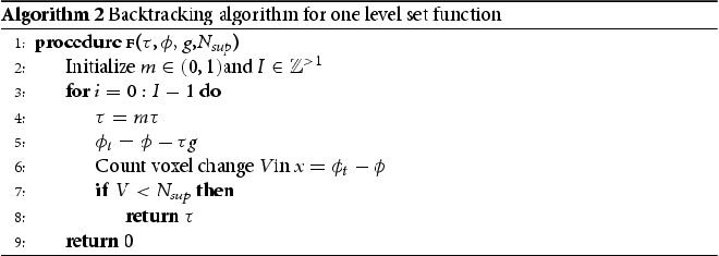
The step size in (EquationA3(A3)
(A3) ) has two components: the first is applied every update (
) and the second is a dynamic scheme which alters the input of
at the end of each sweep.
To begin, we discuss the first component of the scheme. Here, our goal is to choose each entry in such that
(the number of voxels that change per jth source for the mth level set function,
) is contained in an interval which is deemed suitable for the shape associated with the mth level set function to evolve smoothly. The relationship between
and the data misfit is of interest, but as of present is unclear. Although the relationship is unknown, intuition tells us that if we only allow a small amount of voxels to change per update, then we ensure a smooth evolution of the shape which also hopefully induces a smooth evolution of the cost. We choose
, where
is selected appropriately. Typically,
and
is chosen as a small percentage of the total number of voxels in the domain. This quantity gives us a metric for how much each level set function evolves per sweep.
Although the backtracking line search makes sure that updates are only made if , it does not ensure an unequal weighting to each sensitivity pattern generated by the jth source. Ideally, we would like to give greater weighting to those sources which capture objects present in their sensitivity patterns. For example, if we initialize the pth entry in
such that an update to the pth level set function is large, we will consistently accept a voxel change just below
for all sources. This introduces two problems; the first is that more iterations of the backtracking scheme will have to be computed in order to reduce
such that
and the second is that we will give equal weighting to so-called bad updates in the Kaczmarz scheme.
To alleviate this problem, we make use of the quantity . Once a sweep is complete (i.e. we make a Kaczmarz update for each source), we compute the average number of voxels that have changed for that sweep. Mathematically, we have that
(A4)
(A4) This brings us to the second component of the line search criterion. We can adjust
with a weighting vector
, which is chosen by some criterion involving (EquationA4
(A4)
(A4) ). Let us now introduce the subinterval of
, which will be included in our criterion for updating the entries in
:
(A5)
(A5)
(A6)
(A6) where
. From this, we can deduce that
(A7)
(A7) Following this, we adjust each entry in
according to some criterion involving (EquationA4
(A4)
(A4) ), (EquationA5
(A5)
(A5) ), (EquationA6
(A6)
(A6) ). For brevity, we show how the pth component of
is updated per sweep:
(A8)
(A8) where s denotes the quantity for sweep number s.
In other words, this means that if the pth entry to the backtracking line search in Algorithm 2 is too large then this criterion will reduce the step size before it is altered by the backtracking line search. Likewise, if the step size is too low, then this scheme can help the updates become larger. Of course, if entries are extremely large or small, then a scalar multiplier in the intervals given may be insufficient. Nonetheless, the scheme performs reasonably well for our application.
Note that so far, both intervals and
have constant lower and upper bounds. These can be generalized to include bounds which are linearly decreasing dependent on the sweep number. This is not arbitrary, as we expect diminishing returns of gradient descent methods as the sweep number increases. Insisting on the same amount of voxels to be altered later in the algorithm is likely to lead to artefacts in the reconstruction, as the data misfit reduces slower in later iterations. The proportion between
and data misfit should remain the same, which is what these dynamic intervals hope to capture.
Therefore, we introduce a dynamic interval , which induces
. We choose the bounds of
to behave linearly as a function of the sweep number s. It follows that
(A9)
(A9)
(A10)
(A10) where
. Defining the acceptance intervals
and using them for the line search criterion is summarized below:
Choose
and
Determine
Compute
Determine
Use
Use
In the numerical experiments presented in this paper, we have chosen to use the following line search criteria. In the first numerical experiment, we have chosen and in the second
. Note that these numbers for
are not arbitrary; they are chosen as a percentage of the total number of interior cells. Furthermore, we choose
, S = 200 and
for both experiments. Note that here these intervals are constant for each level set function, but other choices are also possible. These are the parameters that define the dynamic intervals described in (EquationA9
(A9)
(A9) ), (EquationA10
(A10)
(A10) ).