Combining adaptive dictionary learning with nonlocal similarity for full-waveform inversion

ABSTRACT

We study the full-waveform inversion (FWI) problem for the recovery of velocity model/image in acoustic media. FWI is formulated as a typical nonlinear optimization problem, many regularization techniques are used to guide the optimization process because the FWI problem is strongly ill-posed. Recently, sparsity regularization has attracted considerable attention in the field of inverse problems. In addition, the nonlocal similarity is also an inherent property of many subsurface images themselves. In this paper, we present a novel computational framework for FWI based on joint local sparsity and nonlocal self-similarity. First, principal component analysis (PCA)-based dictionary learns from noisy approximation images (the estimated results from certain local optimization method) and the learned dictionary is used to guide similar patch grouping. Second, the sparse representation and the nonlocal similarity are introduced as the regularization term. At last, the relative total variation (RTV) algorithm is used to further eliminate the residual artefacts in the reconstructed model more thoroughly. In our inversion strategy, the external optimization knowledge, and the intrinsic local sparsity and nonlocal self-similarity prior of model are used jointly for FWI. Computational results demonstrate the proposed method is obviously superior to existing inversion methods both qualitatively and quantitatively, including total variation FWI method in model-derivative domain and sparsity promoting FWI method in the curvelet domain.

KEYWORDS:

• Full waveform inversion
• principal component analysis (PCA)
• sparse representation
• nonlocal similarity
• relative total variation

2010 MATHEMATICS SUBJECT CLASSIFICATIONS:

• 15A04
• 52A07

1. Introduction

Full-waveform inversion (FWI) is an important imaging modality to retrieve high-resolution velocity model (see [1,2] for a review). FWI relies on a nonlinear least squares optimization problem that attempts minimizing the misfit between recorded and calculated seismic data. The misfit function can be defined in the time domain [3–6] or the frequency domain[7–9] (for further details, please see [10]). Although frequency-domain FWI implementations have various advantages, the insufficiency of the low-frequency information in seismic data, the nonlinearity of the forward model and the ill-posed nature of the formulation all lead to a pressing need for an effective regularization techniques to increase the robustness of FWI and improve inversion quality.

In order to obtain an accurate approximate solution of FWI, the classical Tikhonov regularization is known as one of the most commonly employed methods [11]. However, it leads inversion results to suffer from the over-smoothing effect and be more difficult to recover some small-scale features [12]. Total variation (TV) regularization has been successfully introduced in many different imaging applications, such as image deblurring [13], CT image reconstruction [14], and recovering the salt body through FWI [15,16], because it is able to preserve sharp interfaces and capture some sparsely important information in model-derivative domain. Nevertheless, TV regularization assumes that the model is piecewise smooth, which usually smears out model details and produces staircase artifacts. This effect is due to the fact that TV regularization requires the gradient be sparse and only sharp boundaries be preserved.

Sparsity is a major tool for extracting useful information from indirect measured data, which can provide a more easily interpretable and parsimonious model. Recently, sparsity regularization has attracted great interest in the field of geophysical inverse problems. Successful examples include seismic tomography with the sparsity constraint by using the $l^1$-norm to the model wavelet expansion coefficients [17,18], sparsity constrained FWI using the curvelet or seislet transform [19–22], and the multiple sparsity constraints for FWI [23].

The above mentioned transform domains or dictionaries are analytical and cannot accurately capture the specific structure characteristics of the desired model. In fact, it is very difficult to find a suitable sparse representation for the unknown velocity model with any concise analytical dictionaries because of complicated subsurface structures. A novel, popular, and heart-stirring approach for solving FWI problems is to find the sparse representation of model parameter by using a learned dictionary. Compared with the analytic bases or frames, the learned dictionaries may provide better sparse approximation properties [24], and adapt to patterns in specific problems. Different dictionary learning approaches have already been applied to the sparsity-promoting FWI problem [25–27]. As expected, by learning a set of training data/patches, such dictionaries can provide a more sparse representation of subsurface model parameters.

Based on this and another impressive property called nonlocal similarity, Li and Harris [28] have developed a novel adaptive sparsity-promoting regularization in the model-derivative domain, which unifies the local sparsity and the nonlocal similarity into a variational framework for FWI. In [29], by exploiting nonlocal similarity Shi and Wang presented a novel reverse time migration strategy in seismic imaging. Nonlocal similarity posits that a local patch often has many geometrically similar patches across the model. In the field of image processing, a non-locally centralized sparse representation (NCSR) framework proposed by Dong et al. [30] is very competitive. They exploited the nonlocal similarity to obtain good estimate of the sparse coding coefficients of the clean natural images.

In this paper, to benefit both from the sparsity-based regularization and the nonlocal similarity nature of subsurface model, we propose a new regularization strategy for FWI. Here, the dictionary is trained from PCA transformation, and the PCA-subspace Euclidean distance is used to guide similar patches grouping results, so that the reconstructed model coded by the sub-dictionaries learned from the classified patches can be more sparse. Then, we introduce a nonlocal similarity prior into the sparse representation-based FWI framework. At last, the RTV algorithm is used to further reduce the residual artifacts in the reconstructed model more thoroughly.

In the next section, we briefly review the background of acoustic FWI, and basic optimization algorithms. Section 3 introduces the theoretical details for the proposed method and corresponding numerical scheme. Experimental results are given in Section 4 to demonstrate the advantages of our inversion strategy over FWI with conventional regularization schemes including the TV regularization and sparsity promotion regularization using curvelet transform. Finally, Section 5 presents concluding remarks.

2. Full waveform inversion

The purpose of FWI is to obtain high resolution and precision seismic imaging via minimization of the misfit between observed and forward modeling  data. The observed data is acquired by receiver arrays and denoted as ${\mathbf{d}}_{\mathrm{obs}}$. In the discrete case, $\mathbf{m}\in {\mathbb{R}}^{N_z\times N_x}$ denotes the unknown subsurface model, where $N_z$ and $N_x$ are the number of grid points in z- and x- directions, respectively. In this work, $\mathbf{m}(z_i,x_j)\triangleq 1/\mathbf{v}(z_i,x_j)$ ($\mathbf{v}$ is the discrete velocity model, $i=1,2,\dots ,N_z$, and $j=1,2,\dots ,N_x$) represents the squared-slowness value in a 2D grid. Let $\mathcal{F}(\mathbf{m})$ be the mathematical expression of the forward modelling problem that describes the calculation process from model to data. Therefore, FWI seeks to find a model $\mathbf{m}$ that minimizes the following discrete nonlinear least squares misfit function (1) $\mathrm{\Psi }(\mathbf{m})=\frac{1}{2}\Vert \mathcal{F}(\mathbf{m})-{\mathbf{d}}_{\mathrm{obs}}{\Vert }_F^2,$(1) where $\Vert \cdot {\Vert }_F$ is the Frobenius norm.

In the frequency domain, the forward modeling  operator $\mathcal{F}(\mathbf{m})$ can be obtained by solving the following constant-density Helmholtz equation (2) $A_{\omega }(\mathbf{m})\mathbf{u}=\mathbf{S},$(2) where $A_{\omega }(\mathbf{m})$ is the discretized Helmholtz operator ${\omega }^2\mathbf{m}+{\mathrm{\nabla }}^2$ with perfectly matched layer (PML) boundary conditions for the frequency ω and the model $\mathbf{m}$, the solution $\mathbf{u}$ is the pressure wavefield and $\mathbf{S}$ denotes the source. Let P be a measurement operator that projects the solution $\mathbf{u}$ onto the receiver locations, then the operator $\mathcal{F}(\mathbf{m})$ can be formally written as $P{A}_{\omega }(\mathbf{m}{)}^{-1}\mathbf{S}$.

When a local optimization technique (such as the conjugate gradient method, steepest-descent method or quasi-Newton method) is used to minimize the misfit function in (1(1) $\mathrm{\Psi }(\mathbf{m})=\frac{1}{2}\Vert \mathcal{F}(\mathbf{m})-{\mathbf{d}}_{\mathrm{obs}}{\Vert }_F^2,$(1) ), the gradient of Ψ is required. In this paper, we adopt the L-BFGS algorithm [31], a popular quasi-Newton strategy, which can achieve a much faster convergence speed at minimal computational cost. More specifically, the L-BFGS algorithm iteratively updates the model $\mathbf{m}$ by setting (3) ${\mathbf{m}}_j={\mathbf{m}}_{j-1}-{\tau }_{j-1}{\mathcal{H}}_{j-1}\mathrm{\nabla }\mathrm{\Psi }({\mathbf{m}}_{j-1}),j=1,2,\dots ,$(3) where $\mathrm{\nabla }\mathrm{\Psi }$ is the misfit gradient, it can be calculated by the adjoint-state method [32,33], which specific steps for complex-valued fields can refer to Barucq et al. ([34], Appendix A). Furthermore, the L-BFGS method does not need the complete storage of ${\mathcal{H}}_j$ (an approximation of the inverse Hessian), which is prohibitive for large-scale model. The step length ${\tau }_{j-1}$ is chosen by a line search that satisfies the Wolfe conditions [31,35].

3. The proposed method

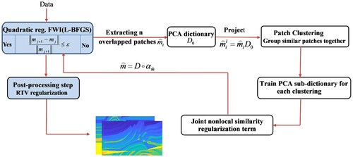
As mentioned above, we need to add sufficient complete prior knowledge of desired model parameters to guide the inversion process to obtain a satisfactory solution. Recently, sparsity-based regularization and nonlocal self-similarity method are becoming more popular in image processing community. In this study, we propose a novel FWI strategy to recover unknown medium parameters properly, aiming to exploit the local sparsity and the nonlocal self-similarity of model parameters simultaneously in a unified framework. The proposed method exploits the PCA sub-dictionaries for adaptive sparse representation and suppresses the sparse coding noise by computing the weighted average of the sparse representation coefficients for nonlocal similar patches to enhance the image quality. We call this method Adaptive Sparse constrained Nonlocal self-Similarity FWI method or ASNS-FWI method for short.

The proposed ASNS-FWI method mainly consists of two loops: In the inner loop, we adopt the L-BFGS algorithm to solve the nonlinear optimization problem (1(1) $\mathrm{\Psi }(\mathbf{m})=\frac{1}{2}\Vert \mathcal{F}(\mathbf{m})-{\mathbf{d}}_{\mathrm{obs}}{\Vert }_F^2,$(1) ), which yields a noisy inversion result. And the outer loop is to obtain an artifact-reduced  result using the Adaptive Sparse constrained Nonlocal self-Similarity (ASNS) method. Most of undesirable artifacts  in the target model are removed after performing the above steps, but there are still some residual streak artifacts . To further remove the residual streak artifacts , the RTV method is introduced as a post-processing step. The following subsections give detail formulation and numerical scheme of the newly proposed ASNS-FWI.

3.1. Sparse representation modeling

While medium parameters are generally not sparse in the ambient domain, most model parameters have a concise representation in the transform domain. Mathematically, the model $\mathbf{m}$ can be sparsely represented as $\mathbf{m}\approx \mathbf{D}\alpha$, by solving the following optimization problem: (4) $\arg \underset{\mathbf{D},\alpha }{min}\Vert \alpha {\Vert }_0,\mathrm{s}.\mathrm{t}.\Vert \mathbf{m}-\mathbf{D}\alpha {\Vert }_2<\epsilon ,$(4) where $\mathbf{D}$ is the dictionary, α is a sparse coefficient vector, $\Vert \alpha {\Vert }_0$ denotes the $l^0$-norm of α, i.e., the number of non-zero components in α, the second term $\Vert \mathbf{m}-\mathbf{D}\alpha {\Vert }_2$ is the $l^2$-norm fidelity term, and $\epsilon >0$ is a small constant.

A crucial question in sparse representation is the choice of the dictionary. Possible choices include various static dictionaries such as discrete cosine transform (DCT), wavelet, and curvelet. Generally, the performance of sparse representation depends on the dictionary used, and most importantly its suitability for the desired model and the problem at hand. In this work, we employ the K-means clustering technique to categorize the extracted image patches into K groups, and use PCA technique to learn a sub-dictionary of each group.

Since the norm $\Vert \cdot {\Vert }_0$ is NP-hard problem, it is usually replaced by the convex norm $\Vert \cdot {\Vert }_1$. For a given dictionary $\mathbf{D}$, we formulate this $l^1$-norm minimization as the following regularization form: (5) ${\alpha }_{\mathbf{m}}=\arg \underset{\alpha }{min}\frac{1}{2}\Vert \mathbf{m}-\mathbf{D}\alpha {\Vert }_2^2+\lambda \Vert \alpha {\Vert }_1.$(5)

In fact, after an estimated result $\hat{\mathbf{m}}$ is obtained by the L-BFGS algorithm, we try to minimize the following optimization problem: (6) ${\alpha }_{\hat{\mathbf{m}}}=\arg \underset{\alpha }{min}\frac{1}{2}\Vert \hat{\mathbf{m}}-\mathbf{D}\alpha {\Vert }_2^2+\lambda \Vert \alpha {\Vert }_1.$(6) To reconstruct the unknown clean model $\mathbf{m}$ based on $\hat{\mathbf{m}}$, some basic notations needed in following analysis are provided.

3.2. PCA dictionary learning

First, we divide the estimated image $\hat{\mathbf{m}}$ from L-BFGS into n overlapped patches of size $\sqrt{P_s}\times \sqrt{P_s}$, where ${\hat{\mathbf{m}}}_i$ represents the image patch at the spatial location i, $i=1,2,\dots ,n$. To remove block artifacts, overlapping patches with a sliding distance of one pixel are used in this paper. Using an extraction matrix ${\mathbf{R}}_i$ to build the connection between $\hat{\mathbf{m}}$ and ${\hat{\mathbf{m}}}_i$, there holds ${\hat{\mathbf{m}}}_i={\mathbf{R}}_i\hat{\mathbf{m}}.$These image patches form a matrix $\mathbf{M}\in {\mathbb{R}}^{P_s\times n}$ given by $\mathbf{M}=[\mathrm{vec}({\hat{\mathbf{m}}}_1),\mathrm{vec}({\hat{\mathbf{m}}}_2),\dots ,\mathrm{vec}({\hat{\mathbf{m}}}_n)],$where $\mathrm{vec}({\hat{\mathbf{m}}}_i)$ is the vectorized model patch. The mean vector of $\mathbf{M}$ is denoted as $\mathbf{d}=E(\mathbf{M})=[d_1,d_2,\dots ,d_n].$Then, we subtract the mean vector $\mathbf{d}$ from $\mathbf{M}$, and $\mathbf{M}$ updates to $\overline{\mathbf{M}}=\mathbf{M}-\mathbf{d}=[\mathrm{vec}({\hat{\mathbf{m}}}_1)-d_1,\mathrm{vec}({\hat{\mathbf{m}}}_2)-d_2,\dots ,\mathrm{vec}({\hat{\mathbf{m}}}_n)-d_n].$The covariance matrix of $\overline{\mathbf{M}}$ can be calculated as $\mathbf{\Omega }=\frac{1}{n-1}\overline{\mathbf{M}}{\overline{\mathbf{M}}}^T.$Because $\mathbf{\Omega }\in {\mathbb{R}}^{P_s\times P_s}$ is symmetrical, its eigenvalue decomposition (EVD) can be written as (7) $\mathbf{\Omega }=\mathbf{\Phi }\mathbf{\Sigma }{\mathbf{\Phi }}^T,$(7) where $\mathbf{\Sigma }\in {\mathbb{R}}^{P_s\times P_s}$ is a diagonal matrix whose diagonal elements $\{{\sigma }_i{\}}_{i=1}^{P_s}$ are the eigenvalues in decreasing order, that is, ${\sigma }_1\ge {\sigma }_2\ge \cdots \ge {\sigma }_{P_s-1}\ge {\sigma }_{P_s}$. The columns of matrix $\mathbf{\Phi }=[{\phi }^{(1)},{\phi }^{(2)},\dots ,{\phi }^{(P_s)}]$ are the corresponding eigenvectors of the covariance matrix $\mathbf{\Omega }$. The energy captured by each eigenvector can be computed as [36] (8) $E_i=\frac{{\sigma }_i}{\sum _{i=1}^{P_s}{\sigma }_i}.$(8) As aforementioned, we adopt PCA to learn the adaptive dictionary. Before that, we can find a proper number d to satisfy $\underset{d\in {\mathbb{N}}^{+}}{min}\{d|\sum _{i=1}^d{E}_i\ge 99\mathrm{\%}\}$. Then, we obtain a PCA dictionary ${\mathbf{D}}_0\in {\mathbb{R}}^{P_s\times d}$ decided by (9) ${\mathbf{D}}_0=[{\phi }^{(1)},{\phi }^{(2)},\dots ,{\phi }^{(d)}],0<d\le P_s.$(9) And using the dictionary ${\mathbf{D}}_0$, we can now project the image patch ${\hat{\mathbf{m}}}_i$ onto this low-dimensional PCA subspace to obtain ${\hat{\mathbf{m}}}_i^l={\hat{\mathbf{m}}}_i{\mathbf{D}}_0$, $i=1,2,\dots ,n$. By applying the K-means clustering algorithm, all patches $\{{\hat{\mathbf{m}}}_i{\}}_{i=1}^n$ can be divided into K groups $\{{\mathbf{G}}_{{\hat{\mathbf{m}}}_i}{\}}_{i=1}^K$. The algorithm requires a similarity metric defined in the sample space, and the Euclidean distance is a usual choice. Recent research [28] has shown that the patch-wise Euclidean distance tends to produce poor results. In our algorithm, we adopt the Euclidean distance in a lower dimensional space determined by PCA to measure the similarity between two image patches. Related concepts are also employed in [37]. For given two image patches ${\hat{\mathbf{m}}}_i$ and ${\hat{\mathbf{m}}}_k$, the PCA subspace Euclidean distance is calculated as (10) ${\mathrm{dis}}_{\mathrm{PCA}}({\hat{\mathbf{m}}}_i,{\hat{\mathbf{m}}}_k)=\Vert {\hat{\mathbf{m}}}_i^l-{\hat{\mathbf{m}}}_k^l{\Vert }_2^2=\sum _{b=1}^d[{\hat{\mathbf{m}}}_{i(b)}^l-{\hat{\mathbf{m}}}_{k(b)}^l{]}^2.$(10) In the work of [37], the theoretical and experimental results for benchmark applications demonstrate that the similarity measure in a low-dimensional subspace described by PCA can capture the intrinsic characteristics of image patches more precisely than in the full space. A major reason for this is that the front few PCA eigenvectors contain important information about the edges or texture of the image patch. 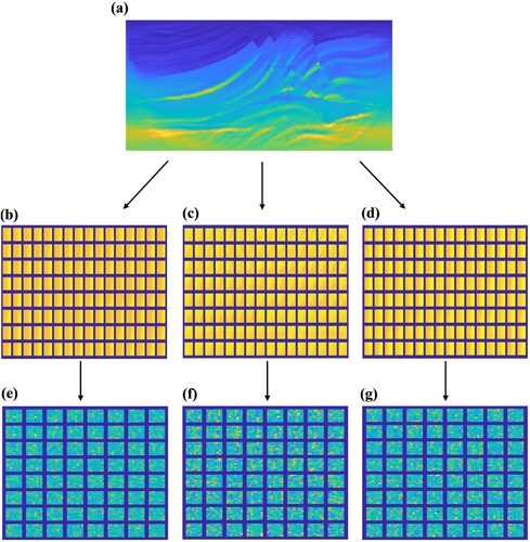For each patch group $\{{\mathbf{G}}_{{\hat{\mathbf{m}}}_i}{\}}_{i=1}^K$, PCA (as shown in formula (9(9) ${\mathbf{D}}_0=[{\phi }^{(1)},{\phi }^{(2)},\dots ,{\phi }^{(d)}],0<d\le P_s.$(9) )) is applied to learn a dictionary $\mathbf{D}\triangleq \{{\mathbf{D}}_i{\}}_{i=1}^K$ called PCA sub-dictionaries. Thanks to the patches in a group are similar to each other, so we construct a set of compact PCA sub-dictionaries for clustered patches rather than an over-complete dictionary. Usually, a compact dictionary will contribute to the decrease of computational cost of the sparse coding for a given image patch [30]. Meanwhile, these K PCA sub-dictionaries construct a large over-complete dictionary to capture all the possible local characteristics of subsurface model. Figures 1 and 2 show examples of three classes of training patches and their corresponding dictionaries.

Figure 1. Three classes of training patches and corresponding dictionaries: (a) the true Marmousi model; (b)–(d) 128 patches from three clusters; (e)–(g) dictionaries trained from corresponding patch clusters.

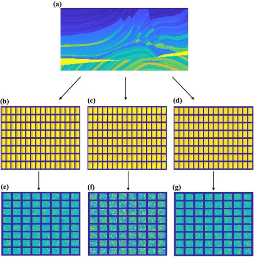
Figure 2. Three classes of training patches and corresponding dictionaries: (a) the inversion result obtained at the end of the first inner loop; (b)–(d) 128 patches from three clusters; (e)–(g) dictionaries trained from corresponding patch clusters.

3.3. Adaptive regularization by nonlocal similarity

Once we obtain the learned dictionary $\mathbf{D}\in {\mathbb{R}}^{P_s\times M}$ ($P_s<M$, M denotes the number of contained atoms in $\mathbf{D}$), each patch ${\hat{\mathbf{m}}}_i$ can be sparsely represented as ${\hat{\mathbf{m}}}_i=\mathbf{D}{\alpha }_{{\hat{\mathbf{m}}}_i}$, and the sparse vector ${\alpha }_{{\hat{\mathbf{m}}}_i}$ can be obtained via solving the following problem: (11) ${\alpha }_{{\hat{\mathbf{m}}}_i}=\arg \underset{{\alpha }_i}{min}\frac{1}{2}\Vert {\hat{\mathbf{m}}}_i-\mathbf{D}{\alpha }_i{\Vert }_2^2+\gamma \Vert {\alpha }_i{\Vert }_1$(11) for some $\gamma >0$.

Then the model image $\mathbf{m}$ is reconstructed as $\mathbf{m}\approx \mathbf{D}\circ {\alpha }_{\hat{\mathbf{m}}}={\left(\sum _{i=1}^n{R}_i^T{R}_i\right)}^{-1}\sum _{i=1}^n(R_i^T\mathbf{D}{\alpha }_{{\hat{\mathbf{m}}}_i}),$where ${\alpha }_{\hat{\mathbf{m}}}$ denotes the concatenation of all ${\alpha }_{{\hat{\mathbf{m}}}_i}\in {\mathbb{R}}^M$, and the notation ° is used to simplify the operation of $(\sum _{i=1}^n{R}_i^T{R}_i{)}^{-1}\sum _{i=1}^n(R_i^T\mathbf{D}{\alpha }_{{\hat{\mathbf{m}}}_i})$. That is, we can express the entire model $\mathbf{m}$ by averaging each recovery patch of ${\hat{\mathbf{m}}}_i$.

Now, the optimization formulation (6(6) ${\alpha }_{\hat{\mathbf{m}}}=\arg \underset{\alpha }{min}\frac{1}{2}\Vert \hat{\mathbf{m}}-\mathbf{D}\alpha {\Vert }_2^2+\lambda \Vert \alpha {\Vert }_1.$(6) ) can be rewritten as (12) ${\alpha }_{\hat{\mathbf{m}}}=\arg \underset{\alpha }{min}\frac{1}{2}\Vert \hat{\mathbf{m}}-\mathbf{D}\circ \alpha {\Vert }_2^2+\gamma \sum _i\Vert {\alpha }_i{\Vert }_1.$(12) Obviously, the sparsity regularization minimization (12(12) ${\alpha }_{\hat{\mathbf{m}}}=\arg \underset{\alpha }{min}\frac{1}{2}\Vert \hat{\mathbf{m}}-\mathbf{D}\circ \alpha {\Vert }_2^2+\gamma \sum _i\Vert {\alpha }_i{\Vert }_1.$(12) ) exploits the local statistics in each image patch. On the other hand, there are usually many repetitive patterns throughout the subsurface model. Such nonlocal redundancy (similarity) is very helpful to increase the quality of reconstructed images. As complementary, by considering redundancy of image patches, a nonlocal similarity is introduced into the minimization problem (12(12) ${\alpha }_{\hat{\mathbf{m}}}=\arg \underset{\alpha }{min}\frac{1}{2}\Vert \hat{\mathbf{m}}-\mathbf{D}\circ \alpha {\Vert }_2^2+\gamma \sum _i\Vert {\alpha }_i{\Vert }_1.$(12) ), in order to make the sparse representation coefficients ${\alpha }_{\hat{\mathbf{m}}}$ close to the true sparse coefficients ${\alpha }_{\mathbf{m}}$ as possible. The sparse coding error (SCN) $\theta ={\alpha }_{\hat{\mathbf{m}}}-{\alpha }_{\mathbf{m}}$ expresses the variation of ${\alpha }_{\hat{\mathbf{m}}}$ from the true sparse coefficients ${\alpha }_{\mathbf{m}}$, which is basically the sparse coding error that obeys the Laplacian distribution [30,37,38]. In practice, ${\alpha }_{\mathbf{m}}$ is unavailable.

Fortunately, there are many similar patterns or structures in the model. First for each local patch ${\hat{\mathbf{m}}}_i$, search Q patches whose PCA-subspace Euclidean distance to its the first-Q smallest compared with all image patches in a large window $L\times L$ centered  at location i. Then, using the selected PCA sub-dictionaries to sparsely represent all patches in $\{{\hat{\mathbf{m}}}_{i,q}{\}}_{q=0}^{Q-1}$, which includes the patch ${\hat{\mathbf{m}}}_i$ itself, i.e. ${\hat{\mathbf{m}}}_i={\hat{\mathbf{m}}}_{i,0}$, and the corresponding sparse coefficients can be calculated as (13) ${\hat{\alpha }}_{i,q}={\mathbf{D}}^T{\hat{\mathbf{m}}}_{i,q},{\hat{\alpha }}_{i,q}\in \{{\hat{\alpha }}_{i,q}{\}}_{q=0}^{Q-1}.$(13) Thus a prediction ${\beta }_i$ of ${\alpha }_{{\mathbf{m}}_i}$ can be calculated by the weighted average of $\{{\alpha }_{i,q}{\}}_{q=0}^{Q-1}$, i.e., (14) ${\beta }_i=\sum _{q=0}^{Q-1}{\omega }_{i,q}{\hat{\alpha }}_{i,q},$(14) where ${\omega }_{i,q}=\exp (-\Vert {\hat{\mathbf{m}}}_{i,q}-{\hat{\mathbf{m}}}_i{\Vert }_2^2/\zeta )/W$, ζ is a predetermined constant, and W is a normalization factor.

By incorporating the nonlocal similarity regularization term, the sparsity regularization minimization (12(12) ${\alpha }_{\hat{\mathbf{m}}}=\arg \underset{\alpha }{min}\frac{1}{2}\Vert \hat{\mathbf{m}}-\mathbf{D}\circ \alpha {\Vert }_2^2+\gamma \sum _i\Vert {\alpha }_i{\Vert }_1.$(12) ) can be rewritten as (15) ${\alpha }_{\hat{\mathbf{m}}}=\arg \underset{\alpha }{min}\frac{1}{2}\Vert \hat{\mathbf{m}}-\mathbf{D}\circ \alpha {\Vert }_2^2+\gamma \sum _i\Vert {\alpha }_i{\Vert }_1+\lambda \sum _i\Vert {\alpha }_i-{\beta }_i{\Vert }_1,$(15) where λ is a regularization parameter. In addition, the sparse coefficient α in equation (15(15) ${\alpha }_{\hat{\mathbf{m}}}=\arg \underset{\alpha }{min}\frac{1}{2}\Vert \hat{\mathbf{m}}-\mathbf{D}\circ \alpha {\Vert }_2^2+\gamma \sum _i\Vert {\alpha }_i{\Vert }_1+\lambda \sum _i\Vert {\alpha }_i-{\beta }_i{\Vert }_1,$(15) ) can be calculated by the PCA sub-dictionaries. The elements of α are zero on $(K-1)$ sub-dictionaries except for the related one and the sparsity is ensured implicitly. Hence, by removing the second term, we can obtain (16) ${\alpha }_{\hat{\mathbf{m}}}=\arg \underset{\alpha }{min}\frac{1}{2}\Vert \hat{\mathbf{m}}-\mathbf{D}\circ \alpha {\Vert }_2^2+\lambda \sum _i\Vert {\alpha }_i-{\beta }_i{\Vert }_1.$(16) Mathematically, the choice of the regularization parameter is critical, and we determine λ by empirical formula as in [38] (17) $\begin{array}{rl}{\lambda }_i& =[{\lambda }_{i_{(1)}},{\lambda }_{i_{(2)}},\dots ,{\lambda }_{i_{(h)}},\dots ,{\lambda }_{i_{(M)}}]\\ & =[\frac{2\sqrt{2}{\sigma }^2}{{\sigma }_{i_{(1)}}},\frac{2\sqrt{2}{\sigma }^2}{{\sigma }_{i_{(2)}}},\dots ,\frac{2\sqrt{2}{\sigma }^2}{{\sigma }_{i_{(h)}}},\dots ,\frac{2\sqrt{2}{\sigma }^2}{{\sigma }_{i_{(M)}}}],\end{array}$(17) in which, let ${\mathrm{\Phi }}_i={\alpha }_{{\hat{\mathbf{m}}}_i}-{\beta }_i$, ${\mathrm{\Phi }}_{i_{(h)}}$ denote the $hth$ element of ${\mathrm{\Phi }}_i$, and ${\sigma }_{i_{(h)}}$ be the standard deviation of ${\mathrm{\Phi }}_{i_{(h)}}$, and σ be the standard deviation of the noise $\hat{\mathbf{m}}-\mathbf{m}$ [37,39]. Even though the true model $\mathbf{m}$ is unknown, according to the above analysis, we can adopt $\mathbf{m}\approx \mathbf{D}\circ {\beta }_{\mathbf{m}}$.

Now for fixed ${\beta }_i$, we solve the following minimization problem: (18) ${\alpha }_{\hat{\mathbf{m}}}=\arg \underset{\alpha }{min}\frac{1}{2}\Vert \hat{\mathbf{m}}-\mathbf{D}\circ \alpha {\Vert }_2^2+\sum _i\sum _h{\lambda }_{i_{(h)}}|{\alpha }_{i_{(h)}}-{\beta }_{i_{(h)}}|.$(18) By utilizing the surrogate algorithm in [40] for solving (18(18) ${\alpha }_{\hat{\mathbf{m}}}=\arg \underset{\alpha }{min}\frac{1}{2}\Vert \hat{\mathbf{m}}-\mathbf{D}\circ \alpha {\Vert }_2^2+\sum _i\sum _h{\lambda }_{i_{(h)}}|{\alpha }_{i_{(h)}}-{\beta }_{i_{(h)}}|.$(18) ), we have (19) ${\alpha }_{i_{(h)}}^{z+1}=S_{\tau }({\alpha }_{i_{(h)}}^z-{\beta }_{i_{(h)}}^z)+{\beta }_{i_{(h)}}^z,$(19) where ${\alpha }_{i_{(h)}}^{z+1}$ is the $hth$ element of ${\alpha }_i$ in the $(z+1)$th iteration, $S_{\tau }(\cdot )$ is the well-known soft-thresholding operator, $\tau ={\lambda }_i/c$, and c is a pre-determined parameter to guarantee the soft-thresholding algorithm convergent. Therefore, the entire model can be reconstructed by (20) $\tilde{\mathbf{m}}\approx \mathbf{D}\circ {\alpha }_{\hat{\mathbf{m}}}.$(20)

3.4. The RTV postprocessing step

The artifacts  of the reconstructed model are greatly removed after implementing the above operator steps, but there are still some residual streak artifacts . In order to remove these artifacts  more thoroughly, the RTV method [41] is used as a postprocessing step. RTV is defined as follows: (21) $\mathrm{RTV}({\mathbf{m}}_p)=\frac{D_x({\mathbf{m}}_p)}{L_x({\mathbf{m}}_p)+ϵ}+\frac{D_y({\mathbf{m}}_p)}{L_y({\mathbf{m}}_p)+ϵ},$(21) where ϵ is a small constant to avoid division by zero. The windowed total variations $D_x({\mathbf{m}}_p)$ and $D_y({\mathbf{m}}_p)$ in two directions for pixel p are expressed as follows: $\begin{array}{rl}{D}_x({\mathbf{m}}_p)& =\sum _{f\in R(p)}{g}_{p,f}\cdot |({\mathrm{\partial }}_x\mathbf{m}{)}_f|,\\ D_y({\mathbf{m}}_p)& =\sum _{f\in R(p)}{g}_{p,f}\cdot |({\mathrm{\partial }}_y\mathbf{m}{)}_f|,\end{array}$where $R(p)$ represents a rectangular region whose central pixel is the pth pixel of model $\mathbf{m}$, the weighting function $g_{p,f}$ is expressed as $g_{p,f}=\exp (-\frac{(x_p-x_f{)}^2+(y_p-y_f{)}^2}{2{\rho }^2})$, and ρ controls the spatial scale of the window.

In addition, the windowed inherent variation (WIV) $L_x({\mathbf{m}}_p)$ and $L_y({\mathbf{m}}_p)$ of the pth pixel are defined as $\begin{array}{rl}{L}_x({\mathbf{m}}_p)& =\sum _{f\in R(p)}|g_{p,f}\cdot ({\mathrm{\partial }}_x\mathbf{m}{)}_f|,\\ L_y({\mathbf{m}}_p)& =\sum _{f\in R(p)}|g_{p,f}\cdot ({\mathrm{\partial }}_y\mathbf{m}{)}_f|.\end{array}$Generally, the WIV values in a rectangular window with more textures are smaller than those in a window with more structures [42]. Therefore, the objective function of RTV regularization is expressed as (22) $\arg \underset{\mathbf{m}}{min}\sum _p\frac{1}{2}\Vert {\mathbf{m}}_p-{\tilde{\mathbf{m}}}_p{\Vert }_2^2+\eta \cdot \sum _p\mathrm{RTV}({\mathbf{m}}_p),$(22) where η is a trade-off parameter. 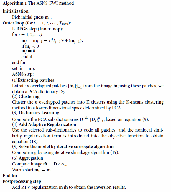In practice, the value of η typically varies in a small interval $[0.01,0.03]$ [41]. So far, the ASNS-FWI method is summarized in the flowchart shown in Figure 3 and the pertinent details of algorithm are given in Algorithm 1.

Figure 3. Flowchart of the ASNS-FWI algorithm.

4. Numerical results

We now present some numerical results to evaluate the performance of the proposed ASNS-FWI method compared to FWI with total variation regularization (TV-FWI) and FWI with curvelet-domain sparsity promotion (CS-FWI) [21]. By adding a regularization term, the misfit function (1(1) $\mathrm{\Psi }(\mathbf{m})=\frac{1}{2}\Vert \mathcal{F}(\mathbf{m})-{\mathbf{d}}_{\mathrm{obs}}{\Vert }_F^2,$(1) ) becomes (23) $\mathrm{\Psi }(\mathbf{m})=\frac{1}{2}\Vert \mathcal{F}(\mathbf{m})-{\mathbf{d}}_{\mathrm{obs}}{\Vert }_2^2+{\lambda }^{\prime }\Vert C\mathbf{m}{\Vert }_1,$(23) where ${\lambda }^{\prime }>0$ is a regularization parameter determined by noise level. Note that if the matrix C represents a discrete gradient operator, the equation (23(23) $\mathrm{\Psi }(\mathbf{m})=\frac{1}{2}\Vert \mathcal{F}(\mathbf{m})-{\mathbf{d}}_{\mathrm{obs}}{\Vert }_2^2+{\lambda }^{\prime }\Vert C\mathbf{m}{\Vert }_1,$(23) ) leads to the well-known TV regularization by using $l^1$-norm term. And if the matrix C is the curvelet transform, the equation (23(23) $\mathrm{\Psi }(\mathbf{m})=\frac{1}{2}\Vert \mathcal{F}(\mathbf{m})-{\mathbf{d}}_{\mathrm{obs}}{\Vert }_2^2+{\lambda }^{\prime }\Vert C\mathbf{m}{\Vert }_1,$(23) ) leads to sparsity promotion regularization by using $l^1$-norm term. To give the best image quality, we have made a lot of numerical experiments. The specific regularization parameter ${\lambda }^{\prime }$ is manually determined in the following example.

In practice, the collected data is often polluted by random noise, so we create a noisy seismic dataset ${\mathbf{d}}_{\mathrm{obs}}$ by adding $1\mathrm{\%}$ white Gaussian noise. The parameter setting is as follows: the model patch size is $\sqrt{P_s}\times \sqrt{P_s}=8\times 8$, the number of similar patches is set to Q = 13, the size of local searching window is $L\times L=25\times 25$, and $\zeta =80$; c = 0.3; $\eta =0.02$. For the ASNS-FWI method, the stopping criteria for the inner loop (L-BFGS iteration) is J = 15 or the objective function (1(1) $\mathrm{\Psi }(\mathbf{m})=\frac{1}{2}\Vert \mathcal{F}(\mathbf{m})-{\mathbf{d}}_{\mathrm{obs}}{\Vert }_F^2,$(1) ) decreases sufficiently small ($\le 1\times {10}^{-5}$). To save computation time, $T_{\max }=4$ outer iterations are performed. The L-BFGS algorithm is used to solve (23(23) $\mathrm{\Psi }(\mathbf{m})=\frac{1}{2}\Vert \mathcal{F}(\mathbf{m})-{\mathbf{d}}_{\mathrm{obs}}{\Vert }_2^2+{\lambda }^{\prime }\Vert C\mathbf{m}{\Vert }_1,$(23) ). Moreover, the L-BFGS algorithm stops if the maximum number $J_{\max }=60$ of iterations is reached, or the misfit function (1(1) $\mathrm{\Psi }(\mathbf{m})=\frac{1}{2}\Vert \mathcal{F}(\mathbf{m})-{\mathbf{d}}_{\mathrm{obs}}{\Vert }_F^2,$(1) ) decrease is small enough ($\le 1\times {10}^{-5}$), which helps to ensure a fair comparison between the proposed ASNS-FWI, TV-FWI and CS-FWI methods. For the CS-FWI method, the fast discrete curvelet transform based on a public code distributed is used [43]. To mitigate the cycle-skipping problem, the inversions are carried out sequentially in 12 overlapping frequency windows on the interval 2–26 Hz.

All the experiments were performed in MATLAB 2018a on a PC equipped with an Intel Core i7-7700 Eight-core (8 Core) 3.60 GHz Processor and 16 GB of RAM. To quantitatively evaluate the performance of different FWI methods, the peak signal-to-noise ratio (PSNR) is commonly used to evaluate the objective image quality, three more powerful reference metrics, the structural similarity index (SSIM), the feature similarity index (FSIM) and the root mean square error (RMSE) are also adopted to evaluate the inversion quality (See Tables 1 and 2).

Table 1. Quantitative results of overthrust model. The brackets represent results without RTV.

		Final results
	Initial	ASNS-FWI	TV-FWI	CS-FWI
SSIM	0.3727	0.7242 (0.6926)	0.5815	0.5641
FSIM	0.8487	0.9817 (0.9811)	0.9549	0.9644
PSNR	9.0064	17.1692 (17.1217)	13.8285	14.5825
RMSE	0.3545	0.1385 (0.1392)	0.2035	0.1865
Running times (s)	–	3092 (3089)	2484	2620

Table 2. Quantitative results of Marmousi model. The brackets represent results without RTV.

		Final results
	Initial	ASNS-FWI	TV-FWI	CS-FWI
SSIM	0.5898	0.7859 (0.7848)	0.7319	0.6320
FSIM	0.8237	0.9729 (0.9724)	0.9416	0.9516
PSNR	17.6142	21.5382 (21.5223)	20.1386	19.3138
RMSE	0.1316	0.0837(0.0839)	0.0986	0.1082
Running times (s)	–	2716 (2712)	2302	2419

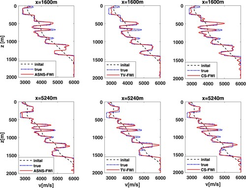
First, the true model (see Figure 4(a)) is a sedimentary part from the Overthrust model. The dimensions of the model are $2010\mathrm{m}\times 8010\mathrm{m}$, with grid spacings of 10 m. The initial velocity model is shown in Figure 4(b). We employ 67 sources and 201 receivers located near the surface and distributed uniformly over the horizontal coordinate. In this experiment, the number of clusters is set to be K = 33. The value of the regularization parameters ${\lambda }^{\prime }$ for the TV-FWI and CS-FWI methods is $1\times {10}^{-4}$. All final inversion results are shown in Figure 4(c)–(f). A direct comparison along vertical logs (as depicted with black dotted line of Figure 4(a)) between the true velocity, the initial and the final velocity models in Figure 5. Clearly, our proposed ASNS-FWI method leads to a more accurate reconstruction in this example. Compared with other two FWI methods, the ASNS-FWI method generates the best visual effect and the structural details of model are better maintained (see red rectangle in Figure 5 (c)–(f). The quantitative evaluation of Overthrust model is given in Table 1. Both subjective visual effects and objective evaluation (except time) criteria clearly show the capability of the proposed ASNS-FWI approach for building high-resolution velocity model.

Figure 4. Inversion results of the Overthrust model: (a) the true velocity model; (b) the initial velocity model; (c) the ASNS-FWI result; (d) the ASNS-FWI result without RTV; (e) the TV-FWI result; (f) the CS-FWI result.

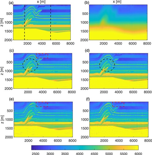
Figure 5. The vertical velocity profiles extracted from the Overthrust model.

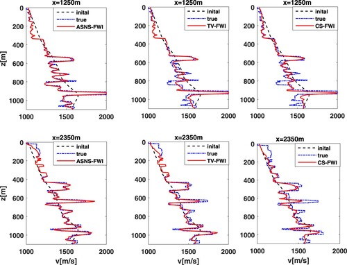
As a second example, we use a modified version of the Marmousi model for numerical tests and true velocity model is shown in Figure 6(a). The initial velocity used to start the FWI is 1-D, which first smoothing the true velocity model with Gaussian kernel, and then averaging along the horizontal direction (Figure 6 (b)). In this example, the model space has $N_z\times N_x=220\times 693$ parameters, with a grid size of 5 m in each direction. As the velocity structure becomes more complex, the number of clusters is K = 64. We set regularization parameters ${\lambda }^{\prime }=1\times {10}^{-3}$ in the TV-FWI and CS-FWI methods. We use 66 equally spaced sources and 198 equally spaced receivers placed near the surface. Final inversion results are shown in Figure 6(c)–(f). Figure 7 depicts two vertical cross-sections through the Marmousi model at x = 1250 m and x = 2350 m (see the black dotted line in Figure 6 (a)). Three FWI methods can give reasonable reconstructions in this example; all main features and interfaces are identified at the correct locations. By examining the results carefully, the proposed ASNS-FWI method restores the fine structure of the model better than other methods (see red rectangles in Figure 6 (c)–(f)). The quantitative results (except time) in Table 2 indicate the improvements of the proposed method are impressive, which together with the visual effect verifies the superiority of the proposed method.

Figure 6. Inversion results of the Marmousi model: (a) the true velocity model; (b) the initial velocity model; (c) the ASNS-FWI result; (d) the ASNS-FWI result without RTV; (e) the TV-FWI result; (f) the CS-FWI result. Note that the total lack of lateral variation in the initial velocity.

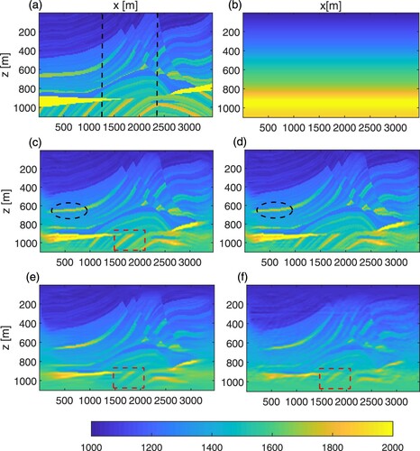
Figure 7. The vertical velocity profiles extracted from the Marmousi model.

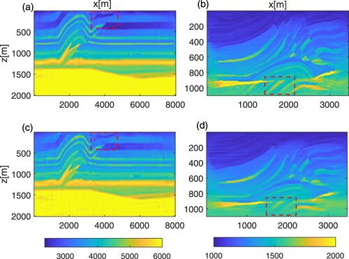
In addition, to demonstrate the impact of RTV postprocessing step on the inversion results, the calculational results of ASNS-FWI method with and without RTV postprocessing steps are presented. The comparison results show that, the residual artifacts  are removed more effectively by using RTV step, which verifies the effectiveness of the RTV in the waveform inversion (see black ellipses in Figures 4 (c),(d) and 6 (c),(d)). To further demonstrate the robustness of our ASNS-FWI method, we add 5% white noise to the seismic data and compare the inversion results of the TV-FWI and ASNS-FWI methods. In our simulations, we take the regularization parameter ${\lambda }^{\prime }=5\times {10}^{-4}$ in the Overthrust model and ${\lambda }^{\prime }=3\times {10}^{-3}$ in the Marmousi model, and the other parameters are chosen be the same as the above experiments. The reconstruction results of TV-FWI and ASNS-FWI methods are shown in Figure 8. In this comparison, we find that the proposed ASNS-FWI method can suppress the random noise more effectively and it helps to obtain a better inversion result (see red rectangles in Figure 8).

Figure 8. Inversion results under 5% white noise in seismic data: (a) the ASNS-FWI result (Overthrust model); (b) the ASNS-FWI result (Marmousi model); (c) the TV-FWI result (Overthrust model); (d) the TV-FWI result (Marmousi model).

There are two major limitations in our FWI method. First, in our experiments, the parameters are manually selected. Therefore, in practice, our method should be combined with other reasonable strategies for parameter selection. A popular machine learning algorithm is a possible solution to adaptively calculate the optimal parameters by learning from an available dataset. Second, due to the introduction of the dictionary learning and nonlocal similarity, the computational complexity of ASNS-FWI is heavier than that of conventional FWI methods. Thus, the use of parallel platforms, including distributed computing, cloud environments, and Graphics Processing Units (GPUs), is vitally important in practice.

5. Conclusion

In this paper, we present a sparsity-based regularization method for FWI that combines the nonlocal similarity prior. The proposed FWI method mainly consists of four stages such as L-BFGS iteration stage, PCA-based dictionary learning stage, nonlocal sparse regularization stage and postprocessing stage. The numerical results of the experimental data show that our inversion method has certain competitiveness compared with existing FWI algorithms. Specifically, ASNS-FWI demonstrates a superior ability to reduce most artifacts  and preserve more structural details. We have also pointed out limitations of the proposed FWI method, and provided some suggestions for practical application. Although we only show FWI examples obtained by acoustic media, our ASNS-FWI can also be applied to elastic media.

Acknowledgments

The authors thank the editor and the anonymous referees for their valuable comments, suggestions and support. This work is partially supported by the National Natural Science Foundation of China (Grant No. 41474102).

Disclosure statement

No potential conflict of interest was reported by the author(s).

Additional information

Funding

The research is supported by the National Natural Science Foundation of China [grant number 41474102].

References

- Virieux J, Stéphane O. An overview of full-waveform inversion in exploration geophysics. Geophysics. 2009;74(6):WCC1–WCC26.
- Wang YH, Rao Y. Reflection seismic waveform tomography. J Geophys Res Solid Earth. 2009;114(B3):B03304.
- Tarantola A. Inversion of seismic reflection data in the acoustic approximation. Geophysics. 1984;49(8):1259–1266.
- Bunks C, Saleck FM, Zaleski S, et al. Multiscale seismic waveform inversion. Geophysics. 1995;60(5):1457–1473.
- Shipp R, Satish CS. Two-dimensional full wavefield inversion of wide-aperture marine seismic streamer data. Geophysical Journal International. 2002;151(2):325–344.
- Han B, Fu HS, Li Z. A homotopy method for the inversion of a two-dimensional acoustic wave equation. Inverse Problems in Science and Engineering. 2005;13(4):411–431.
- Pratt RG, Shin C, Hick GJ. Gauss–Newton and full Newton methods in frequency-space seismic waveform inversion. Geophysical Journal International. 1998;133(2):341–362.
- Brossier R, Operto S, Virieux J. Seismic imaging of complex onshore structures by 2D elastic frequency-domain full-waveform inversion. Geophysics. 2009;74(6):WCC105–WCC118.
- Luo J, Xie X. Frequency-domain full waveform inversion with an angle-domain wavenumber filter. Journal of Applied Geophysics. 2017;141:107–118.
- Wang YH, Rao Y. Waveform Modeling and Tomography. In: Gupta H.K. (eds) Encyclopedia of Solid Earth Geophysics. Encyclopedia of Earth Sciences Series. Springer, Dordrecht; 2021. p. 1608–1621.
- Wang YH. Seismic inversion: theory and applications. Chichester, West Sussex, UK : John Wiley & Sons, Ltd; 2017.
- Aster RC, Borchers B, Thurber CH. Tikhonov regularization. Parameter estimation and inverse problems. 2nd edn; Elsevier Academic Press, New York; 2011. p. 93–127.
- Chan TF, Wong CK. Total variation blind deconvolution. IEEE Transactions on Image Processing. 1998;7(3):370–375.
- Ritschl L, Bergner F, Fleischmann C, et al. Improved total variation-based CT image reconstruction applied to clinical data. Physics in Medicine and Biology. 2011;56(6):1545–1561.
- Esser E, Guasch L, Van Leeuwen T, et al. Total variation regularization strategies in full-waveform inversion. SIAM Journal on Imaging Sciences. 2018;11(1):376–406.
- Peng Y, Liao W, Huang J, et al. Total variation regularization for seismic waveform inversion using an adaptive primal dual hybrid gradient method. Inverse Problems. 2018;34(4):045006.
- Loris I, Nolet G, Daubechies I, et al. Tomographic inversion using l1-norm regularization of wavelet coefficients. Geophysical Journal International. 2007;170(1):359–370.
- Fang H, Zhang H. Wavelet-based double-difference seismic tomography with sparsity regularization. Geophysical Journal International. 2014;199(2):944–955.
- Herrmann FJ, Hanlon I, Kumar R, et al. Frugal full-waveform inversion: from theory to a practical algorithm. Geophysics. 2013;32(9):1082–1092.
- Chai X, Tang G, Peng R, et al. The linearized Bregman method for frugal full-waveform inversion with compressive sensing and sparsity-promoting. Pure Appl Geophys. 2018;175(3):1085–1101.
- Fu HS, Ma MY, Han B. An accelerated proximal gradient algorithm for source-independent waveform inversion. J Appl Geophys. 2020;177:104030.
- Xue Z, Zhu H, Fomel S, et al. Full-waveform inversion using Seislet regularization. Geophysics. 2017;82(5):1–40.
- Peters B, Smithyman BR, Herrmann FJ. Projection methods and applications for seismic nonlinear inverse problems with multiple constraints. Geophysics. 2019;84(2):R251–R269.
- Rubinstein R, Bruckstein AM, Elad M. Dictionaries for sparse representation modeling. Proc IEEE. 2010;98(6):1045–1057.
- Bao C, Cai J, Ji H. Fast sparsity-based orthogonal dictionary learning for image restoration.Sydney, NSW, AustraliaProceedings of the IEEE International Conference on Computer Vision (ICCV).2013.
- Zhu L, Liu E, Mcclellan JH, et al. Sparse-promoting full-waveform inversion based on online orthonormal dictionary learning. Geophysics. 2017;82(2):R87–R107.
- Huang X, Liu Y, Wang F, et al. A robust full waveform inversion using dictionary learning. SEG Technical Program Expanded Abstracts; 2019.
- Li D, Harris JM. Full waveform inversion with nonlocal similarity and model-derivative domain adaptive sparsity-promoting regularization. Geophys J Int. 2018;215(3):1841–1864.
- Shi Y, Wang YH. Reverse time migration of 3D vertical seismic profile data. Geophysics. 2016;18:S31–S38.
- Dong W, Zhang L, Shi G, et al. Image deblurring and super-resolution by adaptive sparse domain selection and adaptive regularization. IEEE Transactions on Image Processing. 2011;20(7):1838–1857.
- Nocedal J, Wright SJ. Numerical optimization. 2nd edn. Berlin, Heidelberg, New York: Springer Verlag; 2006.
- Chavent G. Identification of functional parameters in partial differential equations. IEEE Transactions on Automatic Control. 1974;12(12):155–156.
- Plessix RE. A review of the adjoint-state method for computing the gradient of a functional with geophysical applications. Geophysical Journal International. 2006;167(2):495–503.
- Barucq H, Chavent G, Faucher F, et al. A priori estimates of attraction basins for nonlinear least squares, with application to Helmholtz seismic inverse problem. Inverse Problems. 2019;35(11):115004.
- Metivier L, Brossier R. The seiscope optimization toolbox: a large-scale nonlinear optimization library based on reverse communication. Geophysics. 2016;81(2):F1–F15.
- Reddy SR, Freno BA, Cizmas P, et al. Constrained reduced-order models based on proper orthogonal decomposition. Comput Methods Appl Mech Eng. 2017;321:18–34.
- Wang N, Shi W, Fan C, et al. An improved nonlocal sparse regularization-based image deblurring via novel similarity criteria. Int J Adv Robot Syst. 2018;15(3):172988141878311.
- Liu Q, Zhang C, Guo Q, et al. Adaptive sparse coding on PCA dictionary for image denoising. The Visual Computer. 2016;32(4):535–549.
- Xu J, Zhang L, Zuo W. Patch group based nonlocal self-similarity prior learning for image denoising.Santiago, Chile.In International Conference on Computer Vision.2015.
- Daubechies I, Defrise M, De Mol C, et al. An iterative thresholding algorithm for linear inverse problems with a sparsity constraint. Communications on Pure and Applied Mathematics. 2004;57(11):1413–1457.
- Xu L, Yan Q, Xia Y, et al. Structure extraction from texture via relative total variation. ACM Trans Graph. 2012;31(6):139.
- Gong C, Zeng L. Adaptive iterative reconstruction based on relative total variation for low-intensity computed tomography. Signal Processing. 2019;165:149–162.
- Emmanuel C, Demanet L, Donoho D, et al. Fast discrete curvelet transforms. SIAM J Multiscale Modeling Simul. 2006;5(3):861–899.